Characterization of anomalous diffusion classical statistics powered by deep learning (CONDOR)
←
→
Page content transcription
If your browser does not render page correctly, please read the page content below
Characterization of anomalous diffusion classical
                                                  statistics powered by deep learning (CONDOR)
arXiv:2102.07605v2 [physics.data-an] 8 Apr 2021

                                                                Alessia Gentili, Giorgio Volpe
                                                                Department of Chemistry, University College London, 20 Gordon Street, London
                                                                WC1H 0AJ, UK
                                                                E-mail: g.volpe@ucl.ac.uk

                                                                Abstract. Diffusion processes are important in several physical, chemical, biological
                                                                and human phenomena. Examples include molecular encounters in reactions, cellular
                                                                signalling, the foraging of animals, the spread of diseases, as well as trends in financial
                                                                markets and climate records. Deviations from Brownian diffusion, known as anomalous
                                                                diffusion, can often be observed in these processes, when the growth of the mean square
                                                                displacement in time is not linear. An ever-increasing number of methods has thus
                                                                appeared to characterize anomalous diffusion trajectories based on classical statistics
                                                                or machine learning approaches. Yet, characterization of anomalous diffusion remains
                                                                challenging to date as testified by the launch of the Anomalous Diffusion (AnDi)
                                                                Challenge in March 2020 to assess and compare new and pre-existing methods on three
                                                                different aspects of the problem: the inference of the anomalous diffusion exponent,
                                                                the classification of the diffusion model, and the segmentation of trajectories. Here, we
                                                                introduce a novel method (CONDOR) which combines feature engineering based on
                                                                classical statistics with supervised deep learning to efficiently identify the underlying
                                                                anomalous diffusion model with high accuracy and infer its exponent with a small
                                                                mean absolute error in single 1D, 2D and 3D trajectories corrupted by localization
                                                                noise. Finally, we extend our method to the segmentation of trajectories where the
                                                                diffusion model and/or its anomalous exponent vary in time.

                                                  Keywords: anomalous diffusion, single trajectory characterization, classical statistics
                                                  analysis, supervised deep learning, deep feed-forward neural networks

                                                  1. Introduction

                                                  Anomalous diffusion refers to diffusion phenomena characterized by a mean square
                                                  displacement (MSD) that grows in time with an exponent α that is either smaller
                                                  (subdiffusion) or greater (superdiffusion) than one (standard Brownian diffusion) [1].
                                                  Typically, this is represented by a nonlinear power-law scaling (MSD(t) ∼ tα ) [1].
                                                  The growing interest in anomalous diffusion shown by the physics community lies in
                                                  the fact that it extends the concept of Brownian diffusion and helps describe a broad
                                                  range of phenomena of both natural and human origin [2]. Examples include molecular
Characterization of anomalous diffusion classical statistics powered by deep learning (CONDOR)2

encounters in reactions [3], cellular signalling [4, 5], the foraging of animals [6], search
strategies [7], human travel patterns [8,9], the spread of epidemics and pandemics [10,11],
as well as trends in financial markets [12, 13] and climate records [14].
      Various methods have been introduced over time to characterize anomalous
diffusion in real data. Traditional methods are based on the direct analysis of trajectory
statistics [15] via the examination of features such as the mean square displacement
[16–19], the velocity autocorrelation function [20] and the power spectral density [21,22]
among others [15,23–34]. More recently, the blossoming of machine learning approaches
has expanded the toolbox of available methods for the characterization of anomalous
diffusion with algorithms based on random forests [35,36], gradient boosting techniques
[35], recurrent neural networks [37] and convolutional neural networks [38, 39].
      Despite the significant progress made, the characterization of anomalous diffusion
data still present non-negligible challenges, especially to maintain the approach
insightful, easy to implement and parameter-free [40]. First, the measurement of
anomalous diffusion from experimental trajectories is often limited by the lack of
significant statistics (i.e. single and short trajectories), limited localization precision,
irregular sampling as well as imperceptible time fluctuations and changes in diffusion
properties. Then, these limitations become even more pronounced when dealing
with non-ergodic processes [1], as the information of interest can be well hidden
within individual trajectories. Finally, while machine learning approaches are powerful
and parameter-free, more traditional statistics-based approaches typically offer deeper
insight on the underlying diffusion process.
      These shortcomings have resulted in the launch of the Anomalous Diffusion
(AnDi) Challenge by a team of international scientists in March 2020 (http://www.
andi-challenge.org) [40]. The goal of the challenge was to push the methodological
frontiers in the characterization of three different aspects of anomalous diffusion for 1D,
2D and 3D noise-corrupted trajectories [40]: (1) the inference of the anomalous diffusion
exponent α; (2) the classification of the diffusion model; and (3) the segmentation of
trajectories characterized by a change in anomalous diffusion exponent and/or model at
an unspecified time instant.
      Here, in response to the AnDi Challenge, we describe a novel method
(CONDOR: Classifier Of aNomalous DiffusiOn tRajectories) for the characterization
of single anomalous diffusion trajectories based on the combination of classical statistics
analysis tools and supervised deep learning. Specifically, our method applies a
deep feed-forward neural network to cluster parameters extracted from the statistical
features of individual trajectories. By combining advantages from both approaches
(classical statistics analysis and machine learning), CONDOR is highly performant and
parameter-free. It allows us to identify the underlying anomalous diffusion model with
high accuracy (& 84%) and infer its exponent α with a small mean absolute error
(. 0.16) in single 1D, 2D and 3D trajectories corrupted by localization noise. CONDOR
was always among the top performant methods in the AnDi Challenge for both the
inference of the α-exponent and the model classification of 1D, 2D and 3D anomalous
Characterization of anomalous diffusion classical statistics powered by deep learning (CONDOR)3
Figure 1. Representative anomalous diffusion trajectories. (a-b) Examples
of single 1D anomalous diffusion trajectories in the absence of corrupting noise for (a)
different models of standard diffusion (anomalous diffusion exponent α = 1) and for
(b) the same anomalous diffusion model (sbm) with different values of α. The models
considered here are the annealed transient time motion (attm), the continuous-time
random walk (ctrw), the fractional Brownian motion (fbm), the Lévy walk (lw) and
the scaled Brownian motion (sbm). (c) Same trajectories as in (a) corrupted with
Gaussian noise (of zero mean and variance σn = 1) associated to a finite localization
precision, corresponding to a signal-to-noise ratio (SNR) of 1. For better comparison,
each sequence of positions xn taken at times tn is represented after subtracting its
average and after rescaling its displacements to their standard deviation to give the
normalized sequence x̂n [35]. The grey-shaded areas highlight a small portion (10 data
points) of each trajectory.
diffusion trajectories. In particular, CONDOR was the leading method for the inference
task in 2D and 3D and for the classification task in 3D. Finally, in this article, we extend
CONDOR to the segmentation of trajectories.
2. Methods
CONDOR combines classical statistics analysis of single anomalous diffusion trajectories
with supervised deep learning. The trajectories used in this work are generated
numerically (with the andi-dataset Python package [41]) from the 5 models considered
in the AnDi Challenge: the annealed transient time motion (attm) [42], the continuous-
time random walk (ctrw) [43], the fractional Brownian motion (fbm) [44], the Lévy walk
(lw) [45] and the scaled Brownian motion (sbm) [46]). Briefly, AnDi Challenge datasets
contain 1D, 2D or 3D trajectories from these 5 models sampled at regular time steps
(tn = n∆t, with n a positive integer and ∆t a unitary time interval). The anomalous
exponent α varies in the range [0.05, 2] with steps of 0.05, as allowed by the respective
model [40]. The shortest trajectories have at least 10 samples per dimension (Tmin ).
Prior to the addition of the localization error, the trajectories have a unitary standard
deviation σs of the distribution of the displacements. The trajectories are then corrupted
with additive Gaussian noise (with zero mean and variance σn ) associated to a finite
localization precision to better simulate experimental endeavours [40, 41]. The variance
σn of the Gaussian noise can assume values of 0.1, 0.5 or 1.0 along each directionCharacterization of anomalous diffusion classical statistics powered by deep learning (CONDOR)4
of the trajectories. The final level of noise can be computed as the magnitude of a
vector whose elements are the noise levels along each direction [41]. The inverse of this
value is then used to compute the signal-to-noise ratio (SNR). Figure 1 shows examples
of such trajectories without noise (Figure 1a-b) and with the addition of corrupting
noise (Figure 1c). By visual inspection, these examples show how differences between
single trajectories are not always explicit, thus making the characterization of anomalous
diffusion challenging. Already in the absence of noise, the same diffusion process (e.g.
for α = 1 in Figure 1a) can be described by different models and the same model (e.g.
sbm in Figure 1b) can assume different values of the exponent α. These occurrences
are not always easy to set apart (e.g. attm, fbm and sbm in Figure 1a). The presence
of corrupting noise (Figure 1c) and/or short trajectories (shaded areas in Figure 1a-c)
add extra complexity.
In this section, we provide a detailed description of our method (CONDOR) to
characterise such single anomalous diffusion trajectories. The fundamental intuition
behind our approach is that different trajectories produced by the same diffusion
model should share similar statistical features to set them apart from other models [1].
Nonetheless, in the presence of noise or with few data points, these similarities and
differences do not need be explicit in single trajectories (Figure 1). Thus, CONDOR
first manipulates single trajectories to extract this hidden statistical information and
then employs the power of deep learning to analyse and cluster it. CONDOR workflow is
shown in Figure 2. We will first discuss the feature engineering step used to preprocess
the trajectories and extract a set of N relevant features primarily based on classical
statistics analysis (Section 2.1). These features become the inputs for the deep-learning
part of the characterization algorithm based on deep feed-forward neural networks
(Figure 3), which, in order, classifies the diffusion model and infers the anomalous
diffusion exponent α (Figure 2). These two steps are performed by multiple neural
networks, whose architecture and connection is explained in Section 2.2. Section 2.3
discusses the training of CONDOR neural networks. In Section 2.4, we explain how
CONDOR outputs can be used to perform the segmentation of trajectories, where the
model and/or its anomalous exponent change in time. Finally, in Section 2.5, we provide
a brief explanation of the code behind CONDOR [47].
2.1. Feature engineering and CONDOR input definition
Before the classification and inference steps (Figure 2), we analyzed each trajectory to
extract N = 1 + 92d inputs (with d = 1, 2, 3 being the trajectory dimension) primarily
based on classical statistics (Table 1). The inputs used in this work were ultimately
selected based on the final performance of the deep learning algorithm.
Independently of the dimensionality of the problem, the first input (lnTmax ) is
always connected to the duration Tmax of each trajectory to enable the deep learning
algorithm to properly weight different durations.
To extract the remaining 92d inputs for every trajectory in 1D, 2D and 3D,Characterization of anomalous diffusion classical statistics powered by deep learning (CONDOR)5
Figure 2. CONDOR workflow. CONDOR workflow is divided in three main
parts: preprocessing (Section 2.1), classification and inference (Section 2.2). In the
preprocessing step, the vector of positions x associated to a single trajectory is used
to extract a vector I of N = 1 + 92d inputs primarily based on classical statistics
(with d = 1, 2, 3 being the trajectory dimension). The vector I is the basic input
for each neural network in the classification and inference algorithms. The output of
the classification is determined by the output of up to three deep feed-forward neural
networks and is the predicted model M̃ among five possibile categories: the annealed
transient time motion (attm), the continuous-time random walk (ctrw), the fractional
Brownian motion (fbm), the Lévy walk (lw) and the scaled Brownian motion (sbm).
Finally, the inference algorithm predicts the value of the exponent α ∈ [0.05, 2] basing
its decision on I and the predicted M̃ for each trajectory. In particular, the predicted
α̃ is the arithmetic average of two distinct predictions: α̃1 and α̃2 where M̃ is used as
selection element or additional input for the deep learning algorithm, respectively.
we analysed the vector of the positions along each direction xi ≡ (xi1 , xi2 , .... xiTmax )
∆t
(with i = 1, ... d) independently, after first subtracting its average and rescaling its
displacements wji = xij+1 − xij (with j = 1, ... T∆t max
− 1) to their standard deviation to
i
obtain the normalised displacements ŵj [35]. Practically, for each dimension, this step
produces new time sequences x̂i ≡ (x̂i1 , x̂i2 , .... x̂iTmax ) of positions reconstructed from the
∆t
cumulative sum of the normalised displacements of the original trajectories and with
hx̂i i = 0. Importantly, this step allows for a better comparison between trajectories of
different dimensions and durations while keeping the performance of the deep learning
algorithm optimal [35].
The vectors of the normalised positions x̂i and of the normalised displacements
ŵi ≡ (ŵ1i , ŵ2i , .... ŵiTmax −1 ) are the starting point to calculate the statistical information
∆t
(i.e. the deep learning inputs) associated to each trajectory. In particular, for each
dimension, we calculated the mean (µi ), the median (µi1/2 ), the standard deviation (σ i ),
the skewness (β1i ), the kurtosis (β2i ) and the approximate entropy (ApEni ) associated to
the following (Table 1): the normalised displacements ŵi and the vector of their absolute
i
values Ŵ ≡ (|ŵ1i |, |ŵ2i |, .... |ŵiTmax −1 |), the vector ∆i (m) of the absolute displacements
∆t
∆ij (m) = |x̂ij+m − x̂j | taken at time lags τ = m∆t (with m = 2, 3, ..., T∆t
min
− 1), the
i
ŵj+1
vector ri of the ratios rji = ŵji
, the absolute values |F i {ŵi }| of the normalized Fourier
transform of ŵi , the vector Piδ of the time series of the normalised powers of ŵi segmentsCharacterization of anomalous diffusion classical statistics powered by deep learning (CONDOR)6
Table 1. Statistical information extracted from each dimension of every trajectory
as inputs for the deep learning algorithm. The approximate entropy is introduced as
a way to quantify the amount of regularity and unpredictability of fluctuations over
the considered time series. m = 2, 3, ..., T∆t
min
− 1 and u = 1, 2. Note that ApEni is not
defined for ∆i (m) when m = T∆tmin
− 2 and m = T∆t min
− 1.
i i
ŵi Ŵ ∆i (m) ri |F i {ŵi }| Piδ ∆MSDi |W u {ŵi }|
µi 3 3 3 3 3 3 3
µi1/2 3 3 3 3 3 3 3 3
σi 3 3 3 3 3 3
β1i 3 3 3 3 3 3 3
β2i 3 3 3 3 3 3 3
ApEni 3 3 (3) 3 3 3 3
selected with a non-overlapping moving window of width δ∆t (with δ = 3), the vector
MSDi −MSDi
∆MSDi of the absolute values of the normalised variations ∆MSDij = | j+1
j 2 ∆t2
j
| of
i
the time-averaged mean square displacement (MSD), and the absolute values |W u {ŵi }|
of the wavelet transform of ŵi at the first two translations u∆t with u = 1, 2.
To further improve the performance of the deep learning algorithm, the following
extra four inputs were also added for each dimension to extract additional information
about regular and irregular time patterns in the trajectories (correlations, power
variations and abrupt changes): the integral of the normalized autocorrelation function
(ACF) of ŵi over a time window of width δ∆t to the right of the autocorrelation
peak, the level of frequency asymmetry in the normalized power spectral density of ŵi
calculated as ( T∆t ) 2
P
|F i {ŵi } |2 sgn(k− FN ) with F being the Nyquist frequency, the
max k k 2P N
i
level of time asymmetry in Pδ calculated as k Pδ,k sgn(k − Tmax
i
2δ
), and the occurrence
i
of abrupt changes in the variance of the elements of x̂ [48].
2.2. CONDOR architecture
In the model classification task (Figure 2), the N inputs calculated in the previous step
are first fed to a deep three-layer feed-forward neural network (architecture in Figure 3)
with two sigmoid hidden layers of twenty neurones each and one softmax output layer
of five neurones to predict the model M̃ of anomalous diffusion among the five possible
categories (attm, ctrw, fbm, lw and sbm). We settled for this specific architecture
with two dense layers because it is deep enough to efficiently classify noisy vectors
arbitrarily while still avoiding that its learning rate is slowed down by an excessively
complex architecture. The output of the previous neural network is then refined by
two additional networks with similar architectures (but with three output neurones
and two output neurones, respectively) to improve the classification among trajectories
respectively classified as attm, fbm and sbm and as attm and ctrw (Figure 2), as
these models can be more easily confused. Indeed, in the attm model, the diffusion
coefficient can vary in space or time (in the AnDi challenge only time variations wereCharacterization of anomalous diffusion classical statistics powered by deep learning (CONDOR)7
Inputs Hidden layer 1 Hidden layer 2 Output layer Outputs
Figure 3. Basic neural network architecture in CONDOR. Architecture of
the deep three-layer feed-forward neural network chosen for both classification and
inference tasks. Inputs In (with n = 1, 2, ...N ) are processed by two hidden layers
and an output layer to yield outputs Oq (with q = 1, 2, ...Q).R The hidden layers have
K = 20 neurons each with a sigmoidal activation function ( ). The output layer has
Q neurons with a softmax activation function (σ). Each neuron has a summer (Σ)
that gathers its weighted inputs and bias to return a scalar output. For each neuron,
weights v and bias b are optimised during the training of the network.
considered [40,42]). This feature can be easily confused with features of other processes:
namely, the time-dependent diffusivity of the sbm [46], the time irregularities between
consecutive steps in the ctrw [43] and the correlations among the increments in the
fbm [44].
Once the model is identified, the next step is to infer the anomalous diffusion
exponent α. The estimated value α̃ is obtained as the arithmetic average of the outputs
of two different approaches based on deep learning (Figure 2), as the two approaches
lead to predicting an underestimated α value (α̃1 ) and an overestimated α value (α̃2 ),
respectively. In the first approach (Figure 2), the output M̃ of the classification is used to
cluster the trajectories into five categories based on the identified model. Each category
is analysed independently by a different set of neural networks (architectures as in Figure
3). The neural networks for attm and ctrw have five output categories predicting α̃1
in the range 0.05 to 1 [40, 41]. The neural network for lw has five output categories
predicting α̃1 in the range 1 to 2 [40, 41]. Finally, the prediction for fbm and sbm is
based on a 1x2 directed rooted tree of neural networks with the root network having
two equally spaced output categories predicting α̃1 in the range 0.05 to 2; each category
is then refined by a second neural network with five equally spaced output categories
in the corresponding subrange identified by the root network. In the second approachCharacterization of anomalous diffusion classical statistics powered by deep learning (CONDOR)8
Figure 4. Evolution of CONDOR performance with the size of the training
dataset. (a-c) F1 score calculated on the total 1D, 2D and 3D training datasets of
300k trajectories as a function of the number of trajectories (Nt ) employed to train
the three consecutive networks of the classification task (Figure 2). Nt is normalized
to the size of a single AnDi challenge dataset (Nc = 10k trajectories). The F1 score
is given at the output of (a) the first network, (b) the second network and (c) the
third network used to refine the model predictions in the classification task (Figure 2).
At each of these steps, only the best performing network (black squares) is carried
forward to the next step. (d-e) MAE calculated on the total 1D, 2D and 3D training
datasets of 300k trajectories each as a function of Nt /Nc for (d) α̃1 (dashed lines) and
α̃2 (dotted lines) and (e) for α̃ (solid lines) as defined in Figure 2. For each Nt /Nc , the
arithmetic average α̃ is calculated using the best performing networks used to infer α̃1
and α̃2 with the same number of training trajectories. The networks with the lowest
MAE for α̃1 and α̃2 are also shown in (d) (black circles). The shaded areas correspond
to one standard deviation around the mean values (calculated from the performance
of 5 distinct training attempts).
(Figure 2), the output M̃ of the model classification is used as an additional input
together with the list of inputs identified in Section 2.1. These new set of inputs feed a
1x4 directed rooted tree of neural networks, each with the same overall architecture as in
Figure 3. The root neural network has four equally spaced output categories predicting
α̃2 in the range 0.05 to 2; each of this category is then refined by a second neural network
with five equally spaced output categories in the corresponding α subrange identified
by the root network.
2.3. Training of CONDOR
After defining their architecture, we trained each network of CONDOR independently on
a set of trajectories for which the ground-truth values of the models and of α was known.
Each training was performed using the scaled conjugate gradient backpropagation (scg)
algorithm (for speed) on mixed datasets with up to three hundred thousand trajectories
from different models and values of α, with different durations and levels of corruptingCharacterization of anomalous diffusion classical statistics powered by deep learning (CONDOR)9
noise [41]. Datasets were randomly split among training (70%), validation (15%) and
test (15%) trajectories. Overall, training with scg is very efficient on a standard desktop
computer (processor Intel(R) Core(TM) i7-4790 CPU @ 3.60 GHz), being the size of
the training dataset the main limiting factor. Training the three consecutive networks
used for classification (Figure 2) took at most 1 hour and a half, while training the
fourteen networks for the inference task took at most 3 hours. Training time can be
reduced by up to 2 orders of magnitude employing a GPU. After training, CONDOR is
very computationally efficient on new data. For example, CONDOR can classify ≈ 80k
trajectories/s on a standard desktop computer.
Figure 4 shows the performance of the classification task and of the inference task
with the size of the training dataset. We evaluated the performance of the classification
with the F1 score:
TP
F1 = 1
T P + 2 (F P + F N )
where T P , F P and F N are the true positive, false positive and false negative rates,
respectively. In particular, we computed the micro average of the F1 score with the
Scikit-learn Python’s library [49]. F1 can vary between 0 (no trajectory classified
correctly) and 1 (all trajectories classified correctly). To evaluate the performance of
the inference of the α-exponent, we used the mean absolute error (MAE) instead:
n
1X
MAE = |α̃i − αi |
n i=1
where n is the number of trajectories in the dataset, and α̃i and αi are the predicted
and the ground truth values of the anomalous diffusion coefficient of the i-th trajectory,
respectively. MAE has a lower limit of 0, meaning that the coefficients of all the n
trajectories have been predicted correctly.
Figure 4a-c shows the F1 score measured on the training dataset at the output of the
three consecutive networks used for classification (Figure 2) for the 1D, 2D and 3D cases.
For each step, we increased the number of trajectories used for training progressively
until the F1 score reached near saturation. Past this point any gain in F1 score is
relatively small and by far outbalanced by the increased computational cost associated to
longer training times. The performance improves with the dimension d of the trajectories
and, interestingly, at each step, saturation of the F1 score for higher d appears to take
place with smaller training datasets, as each trajectory contains intrinsically d times
more information. Only the best performing network at each step is selected (black
squares in Figure 2a-c) and carried forward to the next step. Independently of the
dimensionality of the problem, the first network produces the highest increase of F1
score with the size of the training dataset (Figure 4a): for example, going from 10k to
100k trajectories, the F1 score increases approximately by 4% in 1D, 5% in 2D and 6%
in 3D. The combined contribution of the following two networks to the overall F1 score
is less pronounced, especially for higher dimensions (Figure 4b-c); nonetheless they play
a key role in refining the classification among attm, fbm and sbm (Figure 4b) or amongCharacterization of anomalous diffusion classical statistics powered by deep learning (CONDOR)10
attm and ctrw (Figure 4c), thus boosting the final F1 score approximately by 4% in 1D,
3% in 2D and 1% in 3D.
Similarly, Figure 4d-e shows the MAE associated to the inference of the α-exponent
according to α̃1 , α̃2 and their arithmetic average α̃ (as defined in Figure 2) for the 1D,
2D and 3D cases. As for F1 , we report the MAE of each method as a function of the
size of the training dataset progressively until it reaches near saturation. In general, the
MAE lowers with the number of trajectories used for training and with their dimension
d. As noted earlier, independently of the dimensionality of the problem, the arithmetic
average α̃ provides a better estimate of the α exponent with respect to both α̃1 and α̃2 ,
leading to an overall MAE at saturation that is better than those obtained with the
individual methods by at least 0.01 in all the dimensions.
2.4. Segmentation with CONDOR
The output of the classification and the inference can also be used to identify possible
change points in a trajectory. In practice, a trajectory of length Tmax is divided in
Tmax − B + 1 smaller segments using an overlapping moving window of width B (with
BCharacterization of anomalous diffusion classical statistics powered by deep learning (CONDOR)11
Figure 5. CONDOR performance on test datasets. (a) F1 and (b) MAE
obtained using CONDOR on the 1D, 2D and 3D datasets used in the classification and
inference tasks of the AnDi Challenge (10k trajectories each). In (a), the stacked bar
charts shows the contribution of the three consecutive networks used for classification
(Figure 2) to the total F1 score. In (b), the grouped bar charts shows the MAE
associated to the inference of the α-exponent according to α̃1 , α̃2 and their arithmetic
average α̃, which provides the best estimate of the α exponent (Figure 2).
is independent of the deep-learning framework used for its implementation. Moreover,
it is also possible to exchange neural network models between the Deep Learning
ToolboxTM and other platforms, such as those based on TensorFlowTM .
3. Results
3.1. CONDOR overall performance on the datasets of the AnDi Challenge
The best performing networks identified during the training step (black symbols in
Figure 4) were carried forward and used in the prediction step, where we classified the
anomalous diffusion model and inferred the α exponent of the same datasets used in
the AnDi Challenge (with 10k trajectories each) for testing purposes [40]. Figure 5a
shows the overall F1 score obtained on these test databases: F1 = 0.844, F1 = 0.879 and
F1 = 0.913 for the 1D, 2D and 3D cases, respectively. Figure 5b shows the overall MAE
instead: MAE = 0.161, MAE = 0.141 and MAE = 0.121 for the 1D, 2D and 3D cases,
respectively. These very respectable values enabled CONDOR to be one of the top
performant methods in the AnDi Challenge (http://www.andi-challenge.org) [40].
3.2. Analysis of CONDOR performance in the model classification task
Figure 6 provides further detail on CONDOR performance in the classification task
by value of α (Figure 6a-c), by model (Figure 6d), by strength of the localization
noise (Figure 6e) and by trajectory length (Figure 6f-h). These data largely support
CONDOR robustness of performance across the parameter space.Characterization of anomalous diffusion classical statistics powered by deep learning (CONDOR)12
Figure 6. Detailed analysis of CONDOR performance for the classification
task. CONDOR classification performance (F1 score) on the 1D, 2D and 3D datasets
of the AnDi Challenge used for the classification task (as in Figure 5a) (a-c) by value
of α for the (a) 1D, (b) 2D and (c) 3D case, (d) by model, (e) by signal-to-noise
ratio (SNR), and (f-h) by trajectory length for the (f ) 1D, (g) 2D and (h) 3D case,
respectively. In (a-c) each bar corresponds to an increment in α of 0.05. In (a-c) and
(e) the dotted lines represent the overall F1 as in Figure 5a. In (f-h), the trends are
fitted to a power law (y = c − ax−b , with a, b, c > 0) for ease of visualization. The
shaded areas highlight the values of the F1 score above the average value (Figure 5a).
CONDOR is able to predict the correct model relatively consistently across the
values of α, with the exception of α ' 0.05 in 1D and 2D and of α ' 1 for all dimensions
(Figure 6a-c). This is not surprising. In fact, for α ' 0.05 all trajectories are close
to stationary and show a very low degree of motion, which could be dominated by
the localization noise. Therefore, these trajectories are harder to classify, particularly
in lower dimensions where a smaller amount of information is intrinsically available.
Similarly, for α ' 1 all models converge to Brownian motion, making it much more
challenging to distinguish among them. Interestingly, in 1D and 2D, CONDOR
shows an above-than-average performance in classifying superdiffusive trajectories, thus
compensating what lost in the classification of subdiffusive trajectories.
Consistently across the dimensions (1D, 2D and 3D), CONDOR recognises two
models (ctrw and lw) extremely well with F1 ≥ 0.94 for ctrw and F1 ≥ 0.98 for lw
(Figure 6d). This is understandable as both models show typical features that stand
them apart from the remaining models and are relatively robust to the presence of
localization noise (Figure 1): i.e. long ballistic steps in lw trajectories and long waiting
times in ctrw trajectories [1]. For the remaining three models (attm, fbm and sbm),
CONDOR performs progressively better moving from 1D to 3D. As noticed earlier
(Figure 1), the distinctive features among these models are more subtle and can be
better evaluated for higher dimensions as they are intrinsically richer in information
content. While CONDOR performs equally well with fbm and sbm (F1 ≈ 0.81 − 0.82 inCharacterization of anomalous diffusion classical statistics powered by deep learning (CONDOR)13
1D, F1 ≈ 0.85 − 0.86 in 2D and F1 ≈ 0.87 − 0.89 in 3D), it struggles more with attm as
this model can be more easily confused with others (Figure 1). Nonetheless, CONDOR
performance skyrockets with the dimension of the attm trajectories from F1 ≈ 0.66 in
1D to F1 ≈ 0.88 in 3D.
The performance of CONDOR with different values of SNR gives the expected
results (Figure 6e). The F1 score increases for higher values of SNR, reaching F1 scores
of 0.89, 0.92 and 0.95 for 1D, 2D and 3D, respectively (i.e. well above the overall F1
score in Figure 5a). However, even when the noise overcomes the signal (SNR ≤ 1), the
lost in the classification performance is less than 10% of these high values for the level
of noise considered here.
Finally, Figure 6f-h shows CONDOR classification performance with the duration of
the trajectory. Due to the richer information content, classification is increasingly better
for longer trajectories and for higher dimensions. The trends in Figure 6f-h are well fitted
by power law functions (dashed lines), which show how, above a certain threshold in
duration, CONDOR performs above the average F1 scores (delimited by the shaded
areas), reaching F1 values of up to 0.96 in 1D, 0.97 in 2D and 0.99 in 3D. Moreover, this
threshold decreases when increasing the dimension, from ≈ 340 time points in 1D to
≈ 280 in 3D. Note that, by directly training CONDOR neural networks for classification
only with short trajectories (≤ 50 time steps), its performance in classifying them can
be boosted. This possibility is particularly useful for the classification of experimental
trajectories that often are short or are interrupted by missing data points [37, 50]. For
example, we were able to improve the F1 score on short trajectories (≤ 30 time steps)
in Figure 6f-h by ≈ 15% on average.
3.3. Analysis of CONDOR performance in the α-exponent inference task
Figure 7 provides further detail on CONDOR performance in the α-exponent
interference task by value of α (Figure 7a-c), by model (Figure 7d), by strength of
the localization noise (Figure 7e) and by trajectory length (Figure 5f-h). These data
largely confirm the observations on CONDOR performance for the classification task,
thus confirming its robustness across the parameter space.
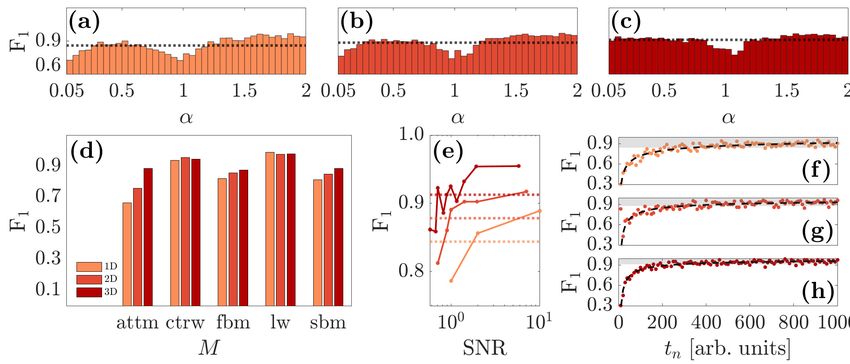
In Figure 7a-c, we can see how CONDOR performs in a relatively consistent way
across the α values, with the exception of α = 0.05 in the 1D and 2D cases (MAE = 0.239
in 1D and MAE = 0.302 in 2D). This is primarily due to a relatively large proportion of
1D and 2D attm trajectories with α = 0.05 being assigned to other α values: for example,
for these trajectories, ≈ 10% of the predicted values of α is greater than 1 (against only
the 0.03% of the 3D attm trajectories with α = 0.05). As in the classification case, being
these subdiffusive trajectories almost stationary, the inference is largely influenced by
the localization noise.
As already noted for the model classification (Figure 6a), CONDOR can also infer
the α-exponent very well and consistently across the dimensions for two models (ctrw
and lw) with MAE ≤ 0.128 for ctrw and MAE ≤ 0.141 for lw (Figure 7d). For the threeCharacterization of anomalous diffusion classical statistics powered by deep learning (CONDOR)14
Figure 7. Detailed analysis of CONDOR performance for the α-exponent
inference task. CONDOR α-exponent inference performance (MAE) on the 1D, 2D
and 3D datasets of the AnDi Challenge used for the inference task (as in Figure 5b)
(a-c) by value of α for the (a) 1D, (b) 2D and (c) 3D case, (d) by model, (e) by
signal-to-noise ratio (SNR), and (f-h) by trajectory length for the (f ) 1D, (g) 2D
and (h) 3D case, respectively. In (a-c) each bar corresponds to an increment in α of
0.05. In (a-c) and (e) the dotted lines represent the overall MAE as in Figure 5b. In
(f-h), the trends are fitted to a power law (y = ax−b + c, with a, b, c > 0) for ease of
visualization. The dashed areas highlight the values of the MAE below the average
value (Figure 5b).
remaining models (attm, fbm and sbm), CONDOR again performs progressively better
moving from 1D to 3D. The best results across the dimensions are obtained for the fbm
(MAE ≈ 0.133 in 1D, MAE ≈ 0.100 in 2D and MAE ≈ 0.083 in 3D), followed by sbm
(MAE ≈ 0.173 in 1D, MAE ≈ 0.134 in 2D and MAE ≈ 0.107 in 3D). Once again, as
in the classification task, CONDOR struggles more with attm (MAE ≈ 0.274 in 1D,
MAE ≈ 0.269 in 2D and MAE ≈ 0.201 in 3D).
Figure 7e confirms what has been discussed for the classification regarding
CONDOR performance with different SNR values. For high SNRs, the MAE values
for each dimension are well below the average MAE (Figure 5b): MAE = 0.136 in 1D,
MAE = 0.121 in 2D and MAE = 0.112 in 3D. As expected, the MAE increases with
higher levels of noise in all dimensions, but it is still below ≈ 0.2 for the values of noise
considered here.
Finally, Figure 7f-h shows CONDOR performance in inferring the α exponent
with the duration of the trajectory. Similar to the classification task, CONDOR
performance improves for higher dimensions and for longer trajectories as the MAE
becomes increasingly lower in agreement with prior observations [35, 37]. The trends
in Figure 7f-h are well fitted by power law functions (dashed lines), which show how,
above a certain threshold in duration, CONDOR performance is significantly below the
average MAE (delimited by the shaded areas), reaching values as small as 0.083 in 1D,Characterization of anomalous diffusion classical statistics powered by deep learning (CONDOR)15 0.085 in 2D and 0.065 in 3D. As for the classification task, this threshold decreases when increasing the dimension, from 350 time points in 1D to 300 in 3D. Also for the inference task, it is possible to improve the prediction of the value of α for short trajectories (≤ 40 time steps) by training CONDOR neural networks only using short trajectories (≤ 50 time steps). Differently from the classification task, training CONDOR on short trajectories does not significantly reduce the error on the inference of the α exponent. 4. Expanding CONDOR to the segmentation of trajectories We tested our algorithm for the segmentation of trajectories on the same datasets used in the AnDi Challenge for the segmentation task [41]. For each dimension, a dataset is composed of 10k trajectories 200 time steps long [40]. Similar to the datasets for the classification and the inference tasks, these datasets are also corrupted by Gaussian noise corresponding to a finite localization precision. Moreover, in these datasets, at least one parameter between the model and the α-exponent changes at a random time ti within the duration of each trajectory. To predict the change point, we used a mov- ing window of width B1 = 50 at first as explained in Section 2.4. We then used two moving windows of width B2 = 40 and B3 = 20 sequentially to refine the prediction of the change point in trajectories where the previous moving window did not detect a change. The results of our segmentation are reported in Figure 8. As shown in Fig- ure 8a, the error in the determination of the change point is strongly influenced by its location in time, reaching its smallest value when the change point is located nearer the center of each trajectory: whilst the overall RMSE for 1D, 2D and 3D trajectories are 53.45, 51.81 and 50.54 respectively, the RMSE reaches average values of 26.00 ± 0.02 in 1D, 24.20 ± 0.04 in 2D and 23.01 ± 0.37 in 3D when the change point is located between 80 and 120 time steps. Interestingly, when the change point location can be determined using larger windows of width B1 (i.e. for 25 < ti < 175), even the overall RMSE is significantly reduced (RMSE equal to 39.38 in 1D, 38.41 in 2D and 36.75 in 3D, Figure 8a), due to CONDOR’s better performance in predicting the model and the α exponent when more time points are available. Once the position of the change point is known, CONDOR can be used to classify the model and infer the α exponent for each segment of the trajectory determined by its segmentation. We either used the networks identified in Figure 4 for long segments (Tmax > 40) or those trained on short trajectories for short segments (Tmax ≤ 40). Figure 8b-c confirms how CONDOR performance in classifying the model and inferring the α exponent increases with the length of the trajectory, which is here determined by the location of the change point in time for each identified trajectory segment. The extra uncertainty introduced by the localization of the change point however leads to slightly lower F1 and slightly higher MAE values across the dimensions with respect to those in Figure 6f-h and Figure 7f-h for trajectories of the same length.
Characterization of anomalous diffusion classical statistics powered by deep learning (CONDOR)16

              Figure 8. Detailed analysis of CONDOR performance for the segmentation
              task. CONDOR segmentation results on the 1D, 2D and 3D datasets of the AnDi
              Challenge used for the segmentation task (10k trajectories each). (a) CONDOR
              segmentation performance is evaluated by the root mean square error (RMSE) of the
              change point localization as a function of the ground truth value of the change point
              (ti ). The dotted lines represent the overall RMSE for each dimension when using
              moving windows of width B1 = 50, B2 = 40 and B3 = 20 sequentially (see text).
              The dash-dotted lines represent the average RMSE for each dimension on all change
              points identified only with a moving window of width B1 (i.e. for 25 < ti < 175).
              (b) Model classification and (c) α-exponent inference with CONDOR on each of the
              two trajectory segments identified through segmentation. These results are reported
              by (b) F1 score and (c) MAE, respectively, for the first (solid lines) and the second
              (dashed lines) trajectory segment as a function of ti .

5. Conclusion

In conclusion, we have introduced a new method (CONDOR) for the characterisation
of single anomalous diffusion trajectories in response to the AnDi Challenge [40]. Our
method combines tools from classical statistics analysis with deep learning techniques.
CONDOR can identify the anomalous diffusion model and its exponent with high
accuracy, in relatively short times and without the need of any a priori information.
Moreover, CONDOR performance is robust to the addition of localization noise.
As a consequence, CONDOR was among the top performant methods in the AnDi
Challenge (http://www.andi-challenge.org), performing pregressively better for
higher dimension trajectories. At the expenses of an increased computational cost,
performance can be further improved by expanding the set of inputs fed to the
deep learning algorithm and by employing more advanced network architectures (e.g.
recurrent neural networks or convolutional neural networks). While most advanced
machine learning techniques often operate as black boxes, we envisage that CONDOR,
being partially based on classical statistics analysis, can help characterise the underlying
diffusion processes with greater physical insight in many real-life phenomena, from
molecular encounters and cellular signalling, to search strategies and the spread of
diseases, to trends in financial markets and climate records.
Characterization of anomalous diffusion classical statistics powered by deep learning (CONDOR)17
Acknowledgements
The authors would like to thank the organisers of the AnDi Challenge for providing a
stimulating scientific environment around anomalous diffusion and its characterization.
The authors acknowledge sponsorship for this work by the U.S. Office of Naval Research
Global (Award No. N62909- 18-1-2170).
References
[1] Ralf Metzler, Jae-Hyung Jeon, Andrey G Cherstvy, and Eli Barkai. Anomalous diffusion models
and their properties: non-stationarity, non-ergodicity, and ageing at the centenary of single
particle tracking. Phys. Chem. Chem. Phys., 16(44):24128–24164, 2014.
[2] Joseph Klafter and Igor M Sokolov. Anomalous diffusion spreads its wings. Phys. World, 18(8):29,
2005.
[3] Eli Barkai, Yuval Garini, and Ralf Metzler. Strange kinetics of single molecules in living cells.
Phys. Today, 65(8):29, 2012.
[4] Felix Höfling and Thomas Franosch. Anomalous transport in the crowded world of biological cells.
Rep. Prog. Phys., 76(4):046602, 2013.
[5] Diego Krapf and Ralf Metzler. Strange interfacial molecular dynamics. Phys. Today, 72(9):48–55,
2019.
[6] Gandhimohan M Viswanathan, Marcos GE Da Luz, Ernesto P Raposo, and H Eugene Stanley. The
physics of foraging: an introduction to random searches and biological encounters. Cambridge
University Press, 2011.
[7] Giorgio Volpe and Giovanni Volpe. The topography of the environment alters the optimal search
strategy for active particles. Proc. Natl. Acad. Sci. U.S.A., 114(43):11350–11355, 2017.
[8] Dirk Brockmann, Lars Hufnagel, and Theo Geisel. The scaling laws of human travel. Nature,
439(7075):462–465, 2006.
[9] Marta C Gonzalez, Cesar A Hidalgo, and Albert-Laszlo Barabasi. Understanding individual human
mobility patterns. Nature, 453(7196):779–782, 2008.
[10] H Zhang and GH Li. Anomalous epidemic spreading in heterogeneous networks. Phys. Rev. E,
102(1):012315, 2020.
[11] Ugur Tirnakli and Constantino Tsallis. Epidemiological model with anomalous kinetics: Early
stages of the covid-19 pandemic. Front. Phys., 8:557, 2020.
[12] Vasiliki Plerou, Parameswaran Gopikrishnan, Luís A Nunes Amaral, Xavier Gabaix, and H Eugene
Stanley. Economic fluctuations and anomalous diffusion. Phys. Rev. E, 62(3):R3023, 2000.
[13] Fredrick Michael and MD Johnson. Financial market dynamics. Physica A, 320:525–534, 2003.
[14] Mozhdeh Massah and Holger Kantz. Confidence intervals for time averages in the presence of
long-range correlations, a case study on earth surface temperature anomalies. Geophys. Res.
Lett., 43(17):9243–9249, 2016.
[15] Yasmine Meroz and Igor M Sokolov. A toolbox for determining subdiffusive mechanisms. Phys.
Rep., 573:1–29, 2015.
[16] Ido Golding and Edward C Cox. Physical nature of bacterial cytoplasm. Phys. Rev. Lett.,
96(9):098102, 2006.
[17] Avi Caspi, Rony Granek, and Michael Elbaum. Enhanced diffusion in active intracellular transport.
Phys. Rev. Lett., 85(26):5655, 2000.
[18] Eldad Kepten, Aleksander Weron, Grzegorz Sikora, Krzysztof Burnecki, and Yuval Garini.
Guidelines for the fitting of anomalous diffusion mean square displacement graphs from single
particle tracking experiments. PLOS One, 10(2):e0117722, 2015.
[19] Xavier Michalet. Mean square displacement analysis of single-particle trajectories with localization
error: Brownian motion in an isotropic medium. Phys. Rev. E, 82(4):041914, 2010.Characterization of anomalous diffusion classical statistics powered by deep learning (CONDOR)18
[20] Stephanie C Weber, Andrew J Spakowitz, and Julie A Theriot. Bacterial chromosomal loci move
subdiffusively through a viscoelastic cytoplasm. Phys. Rev. Lett., 104(23):238102, 2010.
[21] Diego Krapf, Enzo Marinari, Ralf Metzler, Gleb Oshanin, Xinran Xu, and Alessio Squarcini. Power
spectral density of a single brownian trajectory: what one can and cannot learn from it. New
J. Phys., 20(2):023029, 2018.
[22] Diego Krapf, Nils Lukat, Enzo Marinari, Ralf Metzler, Gleb Oshanin, Christine Selhuber-Unkel,
Alessio Squarcini, Lorenz Stadler, Matthias Weiss, and Xinran Xu. Spectral content of a single
non-brownian trajectory. Phys. Rev. X, 9(1):011019, 2019.
[23] Vincent Tejedor, Olivier Bénichou, Raphael Voituriez, Ralf Jungmann, Friedrich Simmel, Christine
Selhuber-Unkel, Lene B Oddershede, and Ralf Metzler. Quantitative analysis of single particle
trajectories: mean maximal excursion method. Biophys. J., 98(7):1364–1372, 2010.
[24] Jae-Hyung Jeon, Natascha Leijnse, Lene B Oddershede, and Ralf Metzler. Anomalous diffusion
and power-law relaxation of the time averaged mean squared displacement in worm-like micellar
solutions. New J. Phys., 15(4):045011, 2013.
[25] Krzysztof Burnecki, Eldad Kepten, Yuval Garini, Grzegorz Sikora, and Aleksander Weron.
Estimating the anomalous diffusion exponent for single particle tracking data with measurement
errors-an alternative approach. Sci. Rep, 5(1):1–11, 2015.
[26] Samudrajit Thapa, Agnieszka Wylomanska, Gregor Sikora, Caroline Wagner, Diego Krapf, Holger
Kantz, Alexei Chechkin, and Ralf Metzler. Leveraging large-deviationstatistics to decipher the
stochastic properties of measured trajectories. New Journal of Physics, 2020.
[27] Konrad Hinsen and Gerald R. Kneller. Communication: A multiscale bayesian inference approach
to analyzing subdiffusion in particle trajectories. J. Chem. Phys., 145(15):151101, 2016.
[28] Natallia Makarava, Sabah Benmehdi, and Matthias Holschneider. Bayesian estimation of self-
similarity exponent. Phys. Rev. E, 84(2):021109, 2011.
[29] Nilah Monnier, Syuan-Ming Guo, Masashi Mori, Jun He, Péter Lénárt, and Mark Bathe. Bayesian
approach to msd-based analysis of particle motion in live cells. Biophys. J., 103(3):616–626,
2012.
[30] Samudrajit Thapa, Michael A Lomholt, Jens Krog, Andrey G Cherstvy, and Ralf Metzler.
Bayesian analysis of single-particle tracking data using the nested-sampling algorithm:
maximum-likelihood model selection applied to stochastic-diffusivity data. Phys. Chem. Chem.
Phys., 20(46):29018–29037, 2018.
[31] Andrey G Cherstvy, Samudrajit Thapa, Caroline E Wagner, and Ralf Metzler. Non-gaussian, non-
ergodic, and non-fickian diffusion of tracers in mucin hydrogels. Soft Matter, 15(12):2526–2551,
2019.
[32] Alexander S Serov, François Laurent, Charlotte Floderer, Karen Perronet, Cyril Favard, Delphine
Muriaux, Nathalie Westbrook, Christian L Vestergaard, and Jean-Baptiste Masson. Statistical
tests for force inference in heterogeneous environments. Sci. Rep, 10(1):1–12, 2020.
[33] Marcin Magdziarz, Aleksander Weron, Krzysztof Burnecki, and Joseph Klafter. Fractional
brownian motion versus the continuous-time random walk: A simple test for subdiffusive
dynamics. Phys. Rev. Lett., 103(18):180602, 2009.
[34] Aleksander Weron, Joanna Janczura, Ewa Boryczka, Titiwat Sungkaworn, and Davide Calebiro.
Statistical testing approach for fractional anomalous diffusion classification. Phys. Rev. E,
99(4):042149, 2019.
[35] Gorka Muñoz-Gil, Miguel Angel Garcia-March, Carlo Manzo, José D Martín-Guerrero, and
Maciej Lewenstein. Single trajectory characterization via machine learning. New J. Phys.,
22(1):013010, 2020.
[36] Joanna Janczura, Patrycja Kowalek, Hanna Loch-Olszewska, Janusz Szwabiński, and Aleksander
Weron. Classification of particle trajectories in living cells: Machine learning versus statistical
testing hypothesis for fractional anomalous diffusion. Physical Review E, 102(3):032402, 2020.
[37] Stefano Bo, Falko Schmidt, Ralf Eichhorn, and Giovanni Volpe. Measurement of anomalous
diffusion using recurrent neural networks. Phys. Rev. E, 100(1):010102, 2019.Characterization of anomalous diffusion classical statistics powered by deep learning (CONDOR)19
[38] Patrycja Kowalek, Hanna Loch-Olszewska, and Janusz Szwabiński. Classification of diffusion
modes in single-particle tracking data: Feature-based versus deep-learning approach. Phys.
Rev. E, 100(3):032410, 2019.
[39] Naor Granik, Lucien E Weiss, Elias Nehme, Maayan Levin, Michael Chein, Eran Perlson, Yael
Roichman, and Yoav Shechtman. Single-particle diffusion characterization by deep learning.
Biophys. J., 117(2):185–192, 2019.
[40] Gorka Muñoz-Gil, Giovanni Volpe, Miguel Angel Garcia-March, Ralf Metzler, Maciej Lewenstein,
and Carlo Manzo. Andi: The anomalous diffusion challenge. arXiv:2003.12036, 2020.
[41] Gorka Muñoz-Gil, Carlo Manzo, Giovanni Volpe, Miguel Angel Garcia-March, Ralf Metzler, and
Maciej Lewenstein. The anomalous diffusion challenge dataset. doi:10.5281/zenodo.370770,
March 2020.
[42] P Massignan, C Manzo, JA Torreno-Pina, MF García-Parajo, M Lewenstein, and GJ Lapeyre Jr.
Nonergodic subdiffusion from brownian motion in an inhomogeneous medium. Phys. Rev. Lett.,
112(15):150603, 2014.
[43] Harvey Scher and Elliott W Montroll. Anomalous transit-time dispersion in amorphous solids.
Phys. Rev. B, 12(6):2455, 1975.
[44] Benoit B Mandelbrot and John W Van Ness. Fractional brownian motions, fractional noises and
applications. SIAM Rev Soc Ind Appl Math, 10(4):422–437, 1968.
[45] J Klafter and G Zumofen. Lévy statistics in a hamiltonian system. Phys. Rev. E, 49(6):4873,
1994.
[46] SC Lim and SV Muniandy. Self-similar gaussian processes for modeling anomalous diffusion. Phys.
Rev. E, 66(2):021114, 2002.
[47] Alessia Gentili and Giorgio Volpe. Classifier of anomalous diffusion trajectories (CONDORv1.0).
doi:10.5281/zenodo.4651470, March 2021.
[48] R. Killick, P. Fearnhead, and I. A. Eckley. Optimal detection of changepoints with a linear
computational cost. J. Am. Stat. Assoc., 107(500):1590–1598, 2012.
[49] F. Pedregosa, G. Varoquaux, A. Gramfort, V. Michel, B. Thirion, O. Grisel, M. Blondel,
P. Prettenhofer, R. Weiss, V. Dubourg, J. Vanderplas, A. Passos, D. Cournapeau, M. Brucher,
M. Perrot, and E. Duchesnay. Scikit-learn: Machine learning in Python. J. Mach. Learn. Res.,
12:2825–2830, 2011.
[50] Johan Elf and Irmeli Barkefors. Single-molecule kinetics in living cells. Annu. Rev. Biochem,
88:635–659, 2019.You can also read