Advances in soil moisture retrieval from multispectral remote sensing using unoccupied aircraft systems and machine learning techniques - HESS
←
→
Page content transcription
If your browser does not render page correctly, please read the page content below

Hydrol. Earth Syst. Sci., 25, 2739–2758, 2021
https://doi.org/10.5194/hess-25-2739-2021
© Author(s) 2021. This work is distributed under
the Creative Commons Attribution 4.0 License.

Advances in soil moisture retrieval from multispectral
remote sensing using unoccupied aircraft systems
and machine learning techniques
Samuel N. Araya1 , Anna Fryjoff-Hung2 , Andreas Anderson2 , Joshua H. Viers2,3 , and Teamrat A. Ghezzehei2,4
1 Earth System Science, Stanford University, Stanford, CA, USA
2 Center for Information Technology in the Interest of Society and the Banatao Institute,
University of California, Merced, Merced, CA, USA
3 Department of Civil and Environmental Engineering, University of California, Merced, Merced, CA, USA
4 Life and Environmental Science, University of California, Merced, Merced, CA, USA

Correspondence: Samuel N. Araya (araya@stanford.edu)

Received: 3 June 2020 – Discussion started: 18 August 2020
Revised: 2 February 2021 – Accepted: 29 March 2021 – Published: 25 May 2021

Abstract. This study investigates the ability of machine          1   Introduction
learning models to retrieve the surface soil moisture of a
grassland area from multispectral remote sensing carried out      The relatively small quantity of water stored in the upper lay-
using an unoccupied aircraft system (UAS). In addition to         ers of the soil plays a key role in terrestrial biology, biogeo-
multispectral images, we use terrain attributes derived from a    chemistry, and atmospheric water and energy fluxes. More
digital elevation model and hydrological variables of precip-     than half of the solar energy absorbed by the land surface is
itation and potential evapotranspiration as covariates to pre-    used to evaporate water (Trenberth et al., 2009), and about
dict surface soil moisture. We tested four different machine      60 % of terrestrial precipitation is returned to the atmosphere
learning algorithms and interrogated the models to rank the       by evapotranspiration (Seneviratne et al., 2010).
importance of different variables and to understand their rela-      In most environments, soil water storage mainly depends
tionship with surface soil moisture. All the machine learning     on precipitation and evapotranspiration (Hillel, 1998; Rana
algorithms we tested were able to predict soil moisture with      and Katerji, 2000), but the distribution of water in the soil
good accuracy. The boosted regression tree algorithm was          is also dependent on soil hydraulic properties, topography,
marginally the best, with a mean absolute error of 3.8 % vol-     and other environmental and belowground conditions (Kor-
umetric moisture content. Variable importance analysis re-        res et al., 2015; Vereecken et al., 2014; Western et al., 1999).
vealed that the four most important variables were precip-        Because of the complex interplay of these variables, it is a
itation, reflectance in the red wavelengths, potential evap-      challenge to accurately estimate soil water. It is typically
otranspiration, and topographic position indices (TPI). Our       impractical to acquire data on soil water dynamics by di-
results demonstrate that the dynamics of soil water status        rect measurement on scales larger than a small experimen-
across heterogeneous terrain may be adequately described          tal plot, and there is no robust approach to predict it. The
and predicted by UAS remote sensing and machine learn-            scarcity of soil moisture data is often cited as a major imped-
ing. Our modeling approach and the variable importance and        iment for the investigation of soil moisture–climate interac-
relationships we have assessed in this study should be use-       tion. Modern techniques for large-scale measurement of soil
ful for management and environmental modeling tasks where         moisture include the cosmic-ray soil moisture observing sys-
spatially explicit soil moisture information is important.        tem (COSMOS)- and the global positioning system interfer-
                                                                  ometric reflectometry (GPS-IR)-based methods. The COS-
                                                                  MOS employs a network of probes across the United States
                                                                  that estimate soil moisture by measuring cosmic-ray neutron

Published by Copernicus Publications on behalf of the European Geosciences Union.
2740                              S. N. Araya et al.: Advances in soil moisture retrieval from multispectral remote sensing

radiation intensity above the land surface (Zreda et al., 2012).   Many studies have focused on deriving surface soil mois-
GPS-based methods are also able to estimate soil moisture          ture content from the synergistic use of remote sensing data
of a few square meters using a GPS signal reflected from the       acquired simultaneously in the optical and thermal infrared
soil. These techniques, while very promising, still need to be     spectrum. The so-called universal triangular relationship is
refined for routine use (Ochsner et al., 2013).                    a widely used method for estimating soil moisture (Nichols
   Remote sensing methods of retrieving soil moisture pro-         et al., 2011; Sobrino et al., 2014).
vide an alternative to conventional methods of soil moisture          Retrieval of information from remote sensing measure-
measurement, which are impractical at large scales. Several        ments is based on the principle that changes in the chemical,
remote sensing methods, particularly from spaceborne de-           physical, and/or structural characteristics of a target deter-
ployment, have been developed to retrieve soil moisture us-        mine the variations in its electromagnetic response (Schanda,
ing optical, thermal infrared, and microwave sensors. Remote       1986). The task of retrieving information from remote sens-
sensing methods enable spatially distributed and frequent ob-      ing is complicated by several factors. Ali et al. (2015) sum-
servations over a large area, which is difficult to achieve        marize the retrieval challenges as being (i) the often complex
when using conventional field measurements (Barrett and            and nonlinear relation between remote sensing measurement
Petropoulos, 2014; Petropoulos et al., 2015). A critical chal-     and target variables of interest; (ii) the ill-posed nature of the
lenge to the current remote sensing methods of retrieving soil     retrieval problem in that electromagnetic response of a tar-
moisture is the lack of imagery with optimum spatial reso-         get is typically the result of contributions from multiple tar-
lutions appropriate for field-scale soil moisture studies and      get variables, and similar electromagnetic responses may be
the low revisit frequency of satellites (Barrett and Petropou-     associated with different physical variables; (iii) the mixed
los, 2014; Das and Mohanty, 2006). Alternatives based on           contribution of multiple objects represented within elemen-
occupied airborne platforms are limited due to their high op-      tary resolution cell; and (iv) the influence of external disturb-
erational costs. Another persistent challenge to soil moisture     ing factors such as noise, radiation components coming from
remote sensing is the difficulty of estimating root zone soil      surrounding of the investigated area, and the atmosphere.
moisture from the surface observations (Nichols et al., 2011;         Soil moisture retrieval from remote sensing has tradition-
Ochsner et al., 2013).                                             ally been done by either empirical approaches or approaches
   Water is one of the most significant chromophores in soils,     based on an inversion of physical models. More recently, the
and studies have shown that narrow band spectral informa-          use of machine learning techniques has gained increased at-
tion in the visible (0.4–0.7 µm), near-infrared (0.7–1.1 µm),      tention because of their ability to tackle many of the limi-
and shortwave infrared (1.1–2.5 µm) regions can be used to         tations with the empirical approaches and physical-model-
estimate surface soil moisture (Ben-Dor et al., 2009; Mal-         based approaches.
ley et al., 2004). Soil reflectance in the visible to short-          Physical-model-based approaches depend on an under-
wave infrared spectral region generally decreases with an          standing of the mechanisms involving the interaction of elec-
increase in soil moisture, with some parts of the spectrum         tromagnetic radiation and the target variable. A wide variety
showing a more pronounced decrease than others (Haubrock           of analytic electromagnetic models have been proposed in
et al., 2008; Weidong et al., 2002). The hydroxide bond is         the literature. The thermal inertia approach (Price, 1977) is
the strongest absorber in the near-infrared region, and free       one such method that is most commonly used for soil mois-
water in soil pores has strong absorption at around the 1.4        ture retrieval using thermal infrared (wavelengths between
and 1.9 µm wavebands (Malley et al., 2004). Several hyper-         3.5 and 14 µm) observation (Barrett and Petropoulos, 2014;
spectral techniques for estimating soil moisture content have      Zhang and Zhou, 2016). Many new soil thermal inertia esti-
been developed, such as the soil moisture Gaussian model           mation methods continue to be developed (Price, 1985; Tian
(SMGM; Whiting et al., 2004) and the normalized soil mois-         et al., 2015; Zhang and Zhou, 2016). The advantages of such
ture index (NSMI; Haubrock et al., 2008).                          physically based models are that they can operate in more
   In the presence of vegetation cover, however, the ability       general scenarios that are difficult to represent through the
to use soil reflectance to measure soil moisture is limited        collection of in situ measurements. However, such models
(Muller and Décamps, 2000). In addition, the reflectance           rely on simplifying the representation of a real phenomenon,
of solar radiation from soil surface represents only about         which can reduce reliability. A major drawback of analyti-
50 µm of the upper soil. This makes it challenging to estimate     cal models is their complexity and requirement for a large
the moisture conditions beneath thin surface layers (Malley        number of input parameters (Zhang and Zhou, 2016).
et al., 2004). Most soil moisture remote sensing approaches           Empirical modeling approaches, on the other hand, em-
operating in the optical range rely on developing an empiri-       ploy statistical regression techniques to develop a mapping
cal spectral vegetation index (Barrett and Petropoulos, 2014).     function based on in situ measurements of the target variable
Several soil moisture measurement methods based on vege-           and corresponding remote sensing measurement. The advan-
tation index proxies have been suggested as vegetation in-         tage of empirical relationships is that they are typically fast
dexes are extremely sensitive to water stress, and they allow      to derive and require fewer inputs. However, such models re-
indirect estimates of soil moisture (Zhang and Zhou, 2016).        quire a higher-quality ground measurement, which could be

Hydrol. Earth Syst. Sci., 25, 2739–2758, 2021                                       https://doi.org/10.5194/hess-25-2739-2021

S. N. Araya et al.: Advances in soil moisture retrieval from multispectral remote sensing                                    2741

time consuming and expensive, and the derived relationship         2     Methods
is typically site and sensor dependent, which limits the pos-
sibility of extending their use readily in a different area (Ali   Multispectral images of the study area were collected on 6
et al., 2015).                                                     different days throughout the 2018 water year using a UAS
   Specific drawbacks to soil moisture remote sensing, using       equipped with a multispectral camera. A high-resolution,
the optical and thermal infrared spectrum, are their shallow       centimeter-scale digital elevation model (DEM) was gen-
soil penetration ability and the cloud-free atmospheric con-       erated from the stereo images using photogrammetric soft-
dition requirement. Many of the optical and thermal infrared       ware, and multiple sets of terrain variables were calculated.
synergistic approaches require a wide range of both vegeta-        Concurrently with the image acquisition flights, the moisture
tion index and soil moisture conditions within a study region,     content of the top 3.8 cm of soil was measured at predefined
which cannot always be satisfied (Barrett and Petropoulos,         sampling locations. The ground soil moisture measurements,
2014).                                                             multispectral reflectance, terrain variables, and rainfall and
   The advantages of machine learning techniques in remote         potential evapotranspiration (PET) data were then aggregated
sensing are their ability to learn and approximate complex         into a data table and used to train a machine learning model
nonlinear mappings and the fact that no assumptions need           to predict the soil moisture. Figure 1 shows the model build-
to be made about data distribution. They can, thus, integrate      ing process.
data from different sources with poorly defined or unknown
probability density functions and have often been shown to         2.1    Study site
outperform other parametric approaches (Ali et al., 2015;
Paloscia et al., 2008). Some of the limitations of machine
learning methods are the need for a large number of training       The study was conducted in a small grassland catchment
data, which require extensive ground truth data sets, and that     at the Merced Vernal Pools and Grassland Reserve located
machine learning methods are black boxes, and only limited         about 5 km northeast of the city of Merced, California. The
inference can be made about the relationships of different in-     grassland is used for livestock grazing; it has a Mediterranean
puts.                                                              climate with hot, dry summers and cool, wet winters, with an
   Remote sensing from unoccupied aircraft systems (UAS)           average annual precipitation of 330 mm (Wong, 2014).
has the potential to address several limitations of traditional       Our study site is a 0.6 km2 area of land located within a
remote sensing. The most attractive feature is their high spa-     subcatchment that contributes to the Avocet Pond, a large
tial resolution, frequent or on-demand image acquisition, and      stock pond located in the northeastern corner of the reserve
low operating costs (Anderson and Gaston, 2013; Berni et al.,      (Fig. 2). The catchment was selected because of an extensive
2009; Colomina and Molina, 2014; Elarab, 2016; Manfreda            hydrologic modeling study that was being conducted on the
et al., 2018; Tmušić et al., 2020). UAS is an umbrella term       site at the time (Fryjoff-Hung, 2018).
that refers to the unoccupied aircraft and the complementary          The study area soils are dominated by Redding grav-
                                                                   elly loam (fine, mixed, active, thermic Abruptic Durixeralfs)
ground control and communication systems necessary for air
surveys (Singh and Frazier, 2018).                                 soils. The elevation of the study area ranges from 118 to
                                                                   162 m above sea level, and the slope ranges from 0 to 31◦ .
1.1   Objectives                                                   The distributions of elevation and slope are shown in Fig. S1
                                                                   in the Supplement.
The purpose of this research was to advance soil moisture             The vernal pool’s ecology is predominantly controlled by
change measurement, process understanding, and prediction          large seasonal shifts and high spatial variability in hydrology;
using remote sensing products from UAS and machine learn-          this makes the study site attractive for our study. UAS remote
ing methods. In this study, the spatial and temporal scale lim-    sensing has the potential to provide information at appropri-
itations were addressed by deploying multispectral remote          ate spatial and temporal scales for vernal pool studies (Stark
sensing with small UAS and surface soil moisture changes           et al., 2015). The annual seasonal cycle of the study site is
were retrieved using machine learning.                             shown in Fig. 3.
   The specific goals of this study were as follows: (1) to
develop an adaptable method for retrieving information on          2.2    Data collection and preparation
surface soil moisture from small UAS remote sensing prod-
ucts and machine learning methods, (2) to identify important       The imagery was acquired on 6 d during the 2018 water year
reflectance and surface characteristics for the prediction of      green-up and brown-down, using a fixed-wing UAS with a
soil moisture changes, (3) to identify appropriate spatial res-    multispectral camera onboard (see Table 3). Figure 4 shows
olutions of reflectance images and terrain variables for esti-     a typical scene of the study site during the wet and dry sea-
mating soil moisture, and (4) to explore the relation of soil      sons. Point soil moisture measurements (top 4 cm) were col-
moisture with surface properties.                                  lected with a time domain reflectometry (TDR) probe across
                                                                   precise sampling transects identified with a real-time kine-

https://doi.org/10.5194/hess-25-2739-2021                                       Hydrol. Earth Syst. Sci., 25, 2739–2758, 2021
2742                              S. N. Araya et al.: Advances in soil moisture retrieval from multispectral remote sensing

Figure 1. Process flowchart of model development.

Figure 2. Map of the Avocet Pond catchment showing the footprint of the study area, ground sampling points, and elevation contours in
meters. Inset shows the location of the study site in California.

matic (RTK) positioning survey. Daily rainfall and PET val-          ground level. Images of a calibrated reflectance panel (Mi-
ues were acquired from nearby weather stations.                      caSense, Inc., Seattle, WA) were taken before each flight and
                                                                     used in the radiometric calibration of the images. The UAS
2.2.1   Image acquisition and processing                             remote sensing flights were conducted between late morn-
                                                                     ings and early afternoons during clear weather conditions.
Multispectral images were acquired using a Parrot Sequoia            A single remote sensing–soil moisture collection campaign
sensor (Parrot SA, Paris, France) equipped with a sunshine           takes between 3 and 4 h. Images were acquired between
sensor that measured irradiance at the sensor spectral wave-         10:00 and 14:00 local time (LT).
bands for radiometric normalization. The camera is deployed             The Parrot Sequoia sensor captures four separable bands in
on a fixed-wing unoccupied aircraft (Finwing Sabre; Finwing          the green, red, red edge, and near-infrared bands, with a fo-
Technology) with an average flight height of 120 m above             cal length of 3.98 mm and resolution of 1280 × 960 pixels. A

Hydrol. Earth Syst. Sci., 25, 2739–2758, 2021                                         https://doi.org/10.5194/hess-25-2739-2021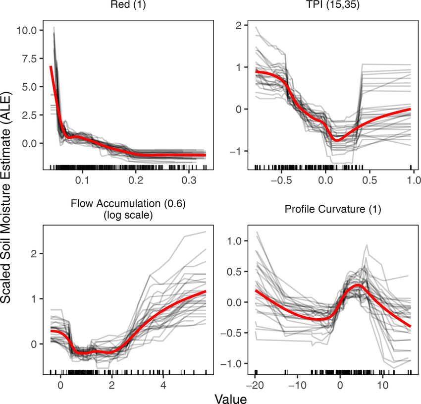
S. N. Araya et al.: Advances in soil moisture retrieval from multispectral remote sensing                                     2743

Figure 3. Vernal pool annual moisture cycle.

                                                                      era’s orientation, the angle of the Sun, and the known re-
                                                                      flectance values of the calibration panel.

                                                                      2.2.2   In situ soil moisture measurement

                                                                      The moisture content of the top 4 cm of soil was measured si-
                                                                      multaneously with UAS remote sensing flights using a Field-
                                                                      Scout TDR 300 soil moisture meter equipped with a 3.8 cm
                                                                      probe (Spectrum Technologies Inc., IL, USA). The Field-
                                                                      Scout TDR 300 measures volumetric water content, using
                                                                      time domain reflectometry, with a resolution of 0.1 % and
Figure 4. Typical scene of the study area in April (a) and June (b)   an accuracy of ± 3 %.
2018.                                                                    Accurate geolocation of the in situ soil moisture measure-
                                                                      ment points is critical for an overlay analysis of the ground
                                                                      measurements with remote sensing products. To ensure ac-
fifth channel captures a high-resolution image in the visible         curate geolocations of the ground measurements, we identi-
spectrum, with a focal length of 4.88 mm and a resolution of          fied six 90 m long sampling transects and recorded the survey
4608 × 3456. Images for the study area were captured with a           grade geolocation of the transect ends using the RTK posi-
minimum of 85 % overlap and a ground pixel resolution of 10           tioning survey. The transect ends were marked with a metal
to 15 cm. Images were scaled to a uniform 15 cm pixel res-            peg hammered into the ground. During each soil moisture
olution during post-processing. Image processing was done             measurement campaign, a 90 m tape measure was temporar-
using Pix4D photogrammetry software (Pix4D, Lausanne,                 ily affixed between the two ends of the transect, and soil
Switzerland). A DEM was photogrammetrically generated                 moisture measurements were taken about every 10 m, not-
from the overlapping stereo images, and images were or-               ing the exact distance of the sampling point from the transect
thorectified and radiometrically calibrated.                          ends.
                                                                         The sampling transects were laid out in a way that ensured
Geometric and radiometric corrections                                 that they run over a variety of topographic variables in terms
                                                                      of flow accumulation, topographic wetness index, and stream
Between seven and nine ground control point (GCP) targets,            networks. Furthermore, each sampling transect fell in a sep-
with precise locations identified by RTK survey, were used            arate subbasin within the Avocet basin.
for photo alignment. The mean georeferencing root mean
square errors (RMSEs) of the GCPs ranged from 0.6 to 2 cm,            2.2.3   Hydrological variables
and the mean reprojection errors ranged from 0.1 to 0.2 px,
based on the bundle block adjustment error assessment re-             Daily precipitation data were retrieved from the University
port. DEM was generated using the structure-from-motion               of California, Merced, weather station located approximately
technique; noise filtering and mild surface smoothing (sharp          6 km southwest of the study site (California Department of
smoothing) were applied to correct for the noisy and erro-            Water Resources, 2018). Daily reference evapotranspiration
neous points of the point cloud. The inverse distance weight-         data were retrieved from the California Irrigation Manage-
ing algorithm was used to interpolate between points to cre-          ment Information System’s (CIMIS) Merced station located
ate the raster DEM.                                                   approximately 10 km south of the study site (California Ir-
   Radiometric calibration by the Pix4D software considers            rigation Management Information System, 2018). The refer-
the positional data, solar irradiance measurements, and gain          ence evapotranspiration is evapotranspiration from standard-
and exposure data from the camera to convert raw digital              ized grass calculated using the modified Penman (CIMIS
numbers into sensor reflectance values. Sensor reflectance            Penman) and Penman–Monteith equations (California Irri-
represents the ratio of the reflected light to the incoming solar     gation Management Information System, n.d.). In this study,
radiation and provides a standardized measure that is directly        we will refer to the reference evapotranspiration as the po-
comparable between images. Finally, surface reflectance is            tential evapotranspiration (PET).
calculated in post-processing, taking into account the cam-

https://doi.org/10.5194/hess-25-2739-2021                                          Hydrol. Earth Syst. Sci., 25, 2739–2758, 2021
2744                              S. N. Araya et al.: Advances in soil moisture retrieval from multispectral remote sensing

2.3     Data processing                                             identify a subset of relevant variables (features) from the
                                                                    larger set of potential predictors. The benefits of variable se-
To prepare the data for machine learning, we compiled all           lection include improvement of model performance, reduc-
the information into a table with the measured soil moisture        ing training and utilization times, and facilitating data under-
from each sampling point and date organized into one col-           standing (Guyon and Elisseeff, 2003; Weston et al., 2003).
umn. Each row contained the accompanying information for            We employed the following three methods of variable se-
that sampling point and time.                                       lection: tests of linear correlation and linear dependencies
                                                                    among variables and recursive feature elimination. Recur-
2.3.1    Feature engineering                                        sive feature elimination involves removing the least impor-
                                                                    tant features whose omission has the least effect on training
We calculated several variables based on the multispectral
                                                                    errors (Chen and Jeong, 2007; Guyon et al., 2002). We imple-
reflectance, terrain, and hydrological data to be used to train
                                                                    mented a recursive feature elimination procedure during the
a machine learning model as predictor variables. A list of all
                                                                    coarse tuning of the boosted regression tree (BRT), random
the measured and calculated variables used in modeling soil
                                                                    forest (RF), artificial neural networks (ANNs), and support
moisture are given in Table 1.
                                                                    vector regression (SVR) algorithm models.
   Topographic variables derived from DEM are scale depen-
                                                                       Following the variable selection procedure, of the 138
dent; to account for this, we calculated all topographic vari-
                                                                    variables, 76 variables were removed based on linear correla-
ables on six DEMs with different resolutions. Prior to calcu-
                                                                    tion and linear dependencies among variables. An additional
lating topographic variables, we upscaled the DEM to 15, 30,
                                                                    16 were removed following the recursive feature elimination
60, 100, 300, and 500 cm cell resolutions and then calculated
                                                                    procedure. The final data used for building the models had
topographic variables for all the resolutions. The calculation
                                                                    46 variables (Table 2), of which five are hydrological, nine
of the topographic position index (TPI) is a special case since
                                                                    are reflectance, and 32 are topographic variables. Variable
it does not only depend on DEM resolution but also on the
                                                                    categories that had no importance included the topographic
definition of the inner and out radii of the annulus (see Eq. 1).
                                                                    wetness index (TWI), the reflectance in the red-edge band,
TPI = Elevation − focal mean (annulus (Inner Radius,                and normalized difference vegetation index (NDVI).
      Outer Radius)).                                        (1)
                                                                    2.4   Data description
   We calculated the TPI for different neighborhood sizes us-       The 6 data collection days in the 2018 water year and sum-
ing the ArcGIS 10.5 Land Facet Corridor tool (Jenness et al.,       mary site statistics are given in Table 3. Cumulative and 30 d
2013). We calculated the TPI on three DEM resolutions (100,         rolling sums of precipitation and PET for the 2018 water year
300, and 500 cm), with two inner radii (1 and 3 cells) and          are shown in Figs. S3 and S4.
three outer radii (3, 5, and 7 cells). A map of selected topo-         Figure 5 shows the distribution of soil moisture and
graphic variables is provided in Fig. S2.                           Thiam’s transformed vegetation index (TTVI) during the 6
   Precipitation and PET are two important drivers of surface       measurement days. The soil moisture measurement followed
soil moisture. To account for antecedent conditions, we used        the general precipitation patterns but was also influenced by
the cumulative water year precipitation and PET and rolling         immediate rainfall events; the highest soil moisture occurred
sums of both variables with different time windows before           on the only measurement day on which it had rained the day
the measurement dates. We calculated cumulative precipita-          before (23 January 2018). The vegetation greenness, as mea-
tion and PET for 1, 2, 3, 7, 15, and 30 d before the sampling       sured with TTVI, followed the 15 d cumulative rainfall well,
dates and used those rolling sums as input.                         with maximum greenness occurring on 4 April 2018 (day
                                                                    of water year 186) and sharply decreasing in the following
2.3.2    Variable selection
                                                                    2 months (Fig. 5).
The total number of soil moisture measurements was 406,                Figure S5 shows the distribution of some terrain vari-
that is, the total number of rows. For each soil moisture           ables associated with the soil moisture sampling points and
point, we added columns with the corresponding date, re-            correlations between variables. The terrain variables for the
flectance, topographic, and hydrological variables. The re-         ground sampling points show a reasonable distribution of
flectance and topographic variables were extracted from the         values, while the distribution of elevation shows a bimodal
raster images using the raster-to-point data extraction tool        distribution with ranges from 120 to 130 m; most of the other
in ArcGIS software, taking the average value of a 1 m di-           variables show a close to normal distribution. The only vari-
ameter buffer around the points. The hydrological variables         ables with Person’s correlation above 0.5 are between TPI
were taken to be the same for the entire study area and only        and curvature (Pearson’s correlation is equal to 0.67). The
changed based on the measurement days.                              distribution of some variables in the data is shown in Fig. S6.
   The data preparation resulted in 138 variables. We em-
ployed variable selection (or feature selections) methods to

Hydrol. Earth Syst. Sci., 25, 2739–2758, 2021                                        https://doi.org/10.5194/hess-25-2739-2021
S. N. Araya et al.: Advances in soil moisture retrieval from multispectral remote sensing                                                                             2745

Table 1. Measured and calculated data used for machine learning. All topographic variables are computed from the digital elevation model.
Descriptions and significance of topographic variables are adapted from Wilson and Gallant (2000).

                     Variable (unit)                            Description                                        Significance or relation to soil mois-
                                                                                                                   ture
                     Soil moisture content (%)                  Volumetric soil moisture content                   Variable of interest
        Measured

                     Daily rainfall (mm)                        Daily rainfall from a precipitation                Source of soil moisture
                                                                gauge (OTT Pluvio) with a wind-
                                                                shield
                     Green (–)                                  Surface reflectance in the green                   Soil and vegetation reflectance
                                                                wavelength band (530–570 nm)                       change
                     Red (–)                                    Surface reflectance in the red wave-               Soil and vegetation reflectance
                                                                length band (640–680 nm)                           change
                     Red edge (–)                               Surface reflectance in the red-edge                Soil and vegetation reflectance
                                                                wavelength band (730–740 nm)                       change
                     Near-infrared (NIR) (–)                    Surface reflectance in the NIR wave-               Soil and vegetation reflectance
                                                                length band (770–810 nm)                           change
                     Altitude (m)                               Elevation (m)                                      Vegetation; potential energy
                     Daily potential evapotranspiration         Reference evapotranspiration from                  Major soil moisture loss pathway
        Calculated

                     (mm)                                       standardized grass calculated using
                                                                CIMIS Penman equation.
                                                                        r
                     Thiam’s transformed vegetation in-         TTVI =       NIR−R
                                                                             NIR+R + 0.5                           Vegetation moisture stress
                     dex (TTVI) (–) ∗
                     Slope (degrees)                            Slope gradient (degrees)                           Surface and subsurface flow velocity,
                                                                                                                   runoff rate, vegetation, geomorphol-
                                                                                                                   ogy
                     Aspect (cos(degree))                       Cosine transformed direction of max-               North- and south-facing slopes dif-
                                                                imum downward gradient (north-                     fer in solar insolation, PET, flora and
                                                                ness)                                              fauna distribution, and abundance
                     Profile curvature (–)                      Downslope curvature                                Flow acceleration, erosion or
                                                                                                                   deposition rate, and geomorphology
                     Plan curvature (–)                         Alongside curvature                                Converging or diverging flow; soil
                                                                                                                   characteristics
                     Tangential curvature (–)                   Curvature in an inclined plane                     Represents areas of convergent (con-
                                                                                                                   cave) and divergent (convex) flow
                     Flow accumulation (multiple flow           Catchment area draining to pixel                   Runoff volume; geomorphology
                     direction, A) (cm2 )
                     Length–slope (LS) factor (–)               Length–slope factor from the Re-                   Calculates a spatially distributed sed-
                                                                vised Universal Soil Loss Equation                 iment transport capacity
                                                                (RUSLE). For slope lengths < 100 m
                                                                and slopes < 14◦ :
                                                                              0.4             1.3
                                                                            A
                                                                LS = 1.4 22.12               S
                                                                                      sin 0.0896

                                                                TPI = Z0 − n1R i∈R Zi
                                                                               P
                     Topographic position index (–)

                     Topographic wetness index (–)                         A
                                                                TWI = ln tan                                       Commonly used index to quantify to-
                                                                             S
                                                                                                                   pographic control on the hydrologi-
                                                                                                                   cal process
      ∗ The TTVI is a transformation of the commonly used normalized difference vegetation index (NDVI). The reason for choosing the TTVI transformation is that it
      eliminates negative values and often transforms NDVI histograms into a more normal distribution. Normalizing machine learning inputs is considered good
      practice and aids models in converging faster.

https://doi.org/10.5194/hess-25-2739-2021                                                                 Hydrol. Earth Syst. Sci., 25, 2739–2758, 2021
2746 S. N. Araya et al.: Advances in soil moisture retrieval from multispectral remote sensing
Table 2. Predictor variables used for machine learning models.
Domain Variable Scale ∗
Hydrological Potential evapotranspiration 1, 30
Precipitation 1, 15, 30
Reflectance Green 0.6, 1, 3
Red 0.6, 1, 3
Near-infrared 0.6, 1, 3
Topographic Northness 0.6, 1, 3, 5
Slope 0.6, 1, 3, 5
Flow direction 0.6, 1, 3, 5
Flow accumulation 0.6, 1, 3, 5
Curvature (profile) 1, 3, 5, 50
Curvature (planform) 0.6, 1, 3, 5, 50
Topographic position index (1,3), (3,7), (3,9), (5,15), (9,21), (15,35), (15,100)
∗ Scale for raster products is pixel resolution in meters and cumulative days for the hydrological variables. Topographic position index
scale is a combination of the inner and outer diameters in meters (see Eq. 1).
Table 3. Data collection days and site summary statistics.
Date Day of the Cumulative Cumulative Mean soil moisture Sample
water year water year water year (and standard
precipitation PET (mm) deviation) (%) count
(mm)
1 30 Oct 2017 30 5.8 96.58 2.47 (1.09) 60
2 4 Dec 2017 65 34.3 149.16 12.26 (5.23) 60
3 23 Jan 2018 115 85.6 199.15 24.85 (7.79) 64
4 4 Apr 2018 186 133.3 371.81 20.27 (10.72) 92
5 1 May 2018 213 177.9 489.18 8.98 (3.93) 74
6 24 May 2018 236 177.9 619.26 4.42 (1.68) 56
2.5 Machine learning procedure where x 0 is the centered and scaled value of variable x, and x
and σx are the arithmetic mean and standard deviation of the
The overall machine learning procedure is illustrated in variable. Standardizing variables prior to model training is
Fig. 1. The computationally demanding steps of model train- a good practice that minimizes issues of scale among input
ing and testing were run at the Multi-Environment Research variables and often leads to better and faster training (Brown-
Computer for Exploration and Discovery (MERCED) high- lee, 2020).
performance computing cluster at the University of Califor-
nia, Merced. The caret R package (v6.0-78; Kuhn, 2008) 2.5.1 Machine learning algorithms used
was used to handle training and tuning procedures. The SVR
and relevance vector regression (RVR) algorithms were im- Several machine learning algorithms exist for multivariate
plemented using the kernlab package (v0.9-26; Karatzoglou regression modeling. Artificial neural networks (ANNs) are
et al., 2004), RF algorithm was implemented using the ran- among the most commonly used algorithms for the retrieval
domForest package (v4.6-12; Liaw and Wiener, 2002), and of soil moisture from remote sensing (e.g., Hassan-Esfahani
the BRT algorithm was implemented using the xgboost pack- et al., 2015; Paloscia et al., 2008). In recent years, the support
age (v0.6.4.1; Chen and Guestrin, 2016). vector machine (SVM) and the similar support vector regres-
Prior to model training, all the predictor variables were sion (SVR) algorithms have become popular in the retrieval
standardized by centering to mean zero and scaling by the of soil moisture (e.g., Ahmad et al., 2010; Zaman and Mc-
variable’s standard deviation (Eq. 2) as follows: kee, 2014; Zaman et al., 2012). Other popular machine learn-
ing algorithms include tree-based models such as the random
x −x forest (RF) and boosted regression trees (BRTs).
x0 = , (2)
σx
Hydrol. Earth Syst. Sci., 25, 2739–2758, 2021 https://doi.org/10.5194/hess-25-2739-2021S. N. Araya et al.: Advances in soil moisture retrieval from multispectral remote sensing 2747
Relevance vector regression (RVR)
Like SVM, the RVR was originally introduced as a classi-
fication machine (Tipping, 2000). RVR is a Bayesian treat-
ment of the SVM prediction function which avoids some of
the limitations of SVM algorithms, such as reducing the use
of basis functions and the need for optimizing the cost and
the insensitivity parameters (Ben-Shimon and Shmilovici,
2006). Torres-Rua et al. (2016) successfully used the RVR
algorithm to estimate surface soil moisture from satellite im-
ages and energy balance products.
Random forest (RF)
RFs are popular models that are relatively simple to train and
tune (Hastie et al., 2009). They apply ensemble techniques by
averaging a large number of individual decision-tree-based
models. Tree models are grown by searching for a predictor
that ensures the best split that results in the smallest model
error. The individual trees in the RF ensemble are built on
a bootstrapped training sample, and only a small group of
predictor variables are considered at each split; this ensures
that trees are decorrelated with each other (Breiman, 2001;
James et al., 2013).
Figure 5. Measured soil moisture and vegetation index of the
ground sampling locations from 1 m resolution raster.
Boosted regression trees (BRTs)
BRT is another form of the decision tree model ensemble
Artificial neural network (ANN)
enhanced by the gradient boosting approach. The gradient
ANN models have been widely used in the development of boosting algorithm constructs additive regression models by
pedotransfer models (Matei et al., 2017; Pachepsky et al., sequentially fitting simple base learner functions (i.e., de-
1996; Schaap et al., 2001; Zhang et al., 2018; Zhang and cision trees) to current pseudo-residuals at each iteration
Schaap, 2017). ANNs are universal approximators that can (Friedman, 2002). These pseudo-residuals are the gradient
approximate any nonlinear mapping. The feed-forward neu- of the loss function being minimized. BRT models have
ral network is a popular variant of ANN. In this study, we shown considerable success and often outperform other ma-
implemented the feed-forward neural network with a single chine learning algorithms in many situations (Elith et al.,
hidden layer, which is considered sufficient for the majority 2008; Natekin and Knoll, 2013). BRT models are also par-
of problems (Reed and Marks II, 1999). ticularly suitable for less-than-clean data (Friedman, 2001),
which makes them particularly attractive in our work where
Support vector regression (SVR) the training data are compiled from various sources and dif-
ferent measurement methods, making them prone to some
SVR is an adaptation of the support vector machine (SVM) inconsistencies.
for regression problems (Cortes and Vapnik, 1995; Drucker Tree-based models, both the RF and BRT, have the advan-
et al., 1997). The SVM learning is a generalization of a max- tage of being able to rank the predictor variable’s relative im-
imal margin classifier. The algorithm first maps the input portance. In these models, the approximate relative influence
variables into a high-dimensional space using a fixed map- of a single predictor variable is calculated as the empirical
ping function, i.e., a kernel function. The algorithm then con- improvement of predictions by splitting on that predictor at
structs hyperplanes, which can be used for classification or, each node and then averaging the relative influence of the
in the case of SVR, for regression. In this study, we use the variable across all trees of the model (Ridgeway, 2012).
radial basis function kernel, which is one of the most-used
kernels in SVR. Some advantages of SVR include the fact 2.5.2 Training–testing set splits
that they do not suffer from the problem of local minima,
and that they have few parameters to tune when training the The data was split into training and testing sets of approxi-
model. mately 75 %–25 %, respectively (i.e., approximately 300 and
100 records). The testing set was a hold-out set used only to
evaluate final trained models.
https://doi.org/10.5194/hess-25-2739-2021 Hydrol. Earth Syst. Sci., 25, 2739–2758, 20212748 S. N. Araya et al.: Advances in soil moisture retrieval from multispectral remote sensing
The training–testing set splitting was done based on a ran- N
1 X
dom selection of the transect. For the testing set, two tran- MBE = (yˆi − yi ) (4)
N i=1
sects are randomly selected on four randomly selected sam- PN 2
pling dates, and one transect is randomly selected on the 2 i=1 yi − yˆi
remaining two sampling dates. To minimize the bias that R = 1 − PN 2
, (5)
i=1 (yi − y)
may result from the training–testing set split, we generated
30 unique training–testing set splits and trained 30 separate where N is the number of observations, y is the measured
models based on each separate training set. The performance value, ŷ is the predicted value, and y is the mean of measured
of each model was assessed on its respective testing set. Sim- values.
ilar performance of the individual models would indicate that The MAE indicates the average deviation of predictions
bias due to the training–testing set split is minimal. The justi- from the measured value, with smaller values indicating bet-
fication for this subsetting procedure is as follows: (1) the se- ter performance. The MBE measures the average system-
lection of entire transects as testing sets avoids possible data atic bias, and positive or negative values indicate the aver-
leakage between the training and testing sets due to spatial age tendency of the predicted values to be larger or smaller
autocorrelation since samples in a transect are located close than the measured values, respectively. The R 2 measures the
to each other – a simple random splitting would not avoid correspondence between predicted and measured data, with
this potential problem; (2) all six sampling dates are repre- higher values indicating stronger correspondence. The MAE
sented in the training set – models are trained on the entire was chosen over RMSE as it is a more appropriate measure
range of time and soil moisture changes; and (3) the testing when averaging (Willmott and Matsuura, 2005).
set is between 25 % and 30 % of the data (between 100 and
Variable importance
125 samples).
The distribution of samples across the sampling dates and The predictor variable importance is the statistical signifi-
transects for the training and testing sets is shown in Figs. S7 cance of each predictor variable with respect to its effect on
and S8, respectively. On average, the training–testing split the generated model. For the tree-based models, RF and BRT,
was 294 samples in the training sets and 113 samples in the variable importance is calculated internally within the model
testing sets. All the training sets have samples from all the algorithm. For the rest of the machine learning models, we
six sampling dates and transects. While all sampling dates calculated the predictor variable importance by the recursive
are represented in each testing set, on average, there are five feature elimination method, which is done by recursively re-
transects in each testing set. moving predictors before training a model and evaluating the
change in model performance. In this method, to account
2.5.3 Cross-validation procedure
for possible bias in variable subset selection (Ambroise and
The selection of optimal model parameters in the model McLachlan, 2002; Hastie et al., 2009), we included a sepa-
training process was done by the cross-validation method. rate layer of 10-fold cross validation in the entire sequence
Cross validation is done to estimate the test error rate by modeling steps.
holding out a subset of the training data (i.e., a validation set)
Effect of predictor variables
from the fitting process and then applying the fitted model to
predict the validation subset. A 30-fold cross-validation set The relationship between the predictor variables and out-
was generated by randomly splitting the training data into puts for a black box model can be analyzed using model-
80 %–20 % training–validation split by randomly selecting a independent methods such as partial dependence plots or ac-
single transect every day. Optimum model parameters were cumulated local effects (ALEs) plots (Apley and Zhu, 2020;
selected using a comprehensive grid search method. Greenwell, 2017). These plots help to explain the relation-
ship between the outcome of the black-box-supervised ma-
2.5.4 Model assessment
chine learning models and the predictors of interest. We use
Performance the ALE plots to analyze the effect of selected predictor vari-
ables. Although similar, the ALE plots are preferred over
The final performance of models was assessed on the sep- partial dependence plots for their speed and their ability to
arate hold-out test data set that was not used in the model produce unbiased plots when variables are correlated (Apley
training. The performance of models is measured in terms of and Zhu, 2020). The value of the ALE is centered so that the
mean absolute error (MAE), mean bias error (MBE), and the mean effect is zero; it can be interpreted as being the effect
coefficient of determination (R 2 ) determined as follows: of the variable on the outcome at a certain value compared
to the average prediction of the data. For example, if an ALE
N
1 X estimate of −2 occurs when a variable of interest has a value
MAE = |yi − ŷi | (3) of 3, then the prediction is lower by 2 compared to the aver-
N i=1
age prediction (Molnar, 2019).
Hydrol. Earth Syst. Sci., 25, 2739–2758, 2021 https://doi.org/10.5194/hess-25-2739-2021S. N. Araya et al.: Advances in soil moisture retrieval from multispectral remote sensing 2749
higher soil moisture levels. In addition, the model prediction
appears capped at around 40 % soil moisture content; this is
likely the result of a lack of training data points with values
above that soil moisture (see Fig. 5). The marginal box plot
on the y axis of Fig. 7 illustrates this point as values above a
40 % soil moisture content are over 1.5 times the interquartile
range above the upper quartile and are plotted as outliers.
Figure 6. Distribution of residuals and MAE on the testing set by 3.2 Predictor variable importance
the type of machine learning algorithm. Filled circles and values to
the right indicate the average MAE. Precipitation and PET were among the top variables in terms
of predictive importance. This is to be expected, given that
these two variables represent the major source and loss path-
3 Results and discussion way for surface soil moisture. Reflectance in the red band
was by far the most important of all the reflectance bands.
3.1 Model performance Following these three variables, topographic variables – TPI
and curvature in particular – were most important in most
All the tested machine learning algorithms were able to pre- models. Topography has a strong control on soil moisture
dict soil moisture with good accuracy. Both BRT and RF al- distribution at landscape scales (Sørensen et al., 2006), while
gorithms, however, had a slightly better performance with a the TPI was the most important topographic variable in de-
MAE of less than 4 % soil moisture content. Figure 6 shows termining soil moisture. A surprising finding was that TWI
the performances of the five machine learning algorithms in was found not to be an important predictor despite numerous
the testing set. The relatively better performance of BRT and studies finding it important in explaining surface soil mois-
RF models is consistent with other studies that find that en- ture (e.g. Moore et al., 1988; Western et al., 1999) Despite
semble decision-tree-based regression models perform bet- calculating TWI in multiple ways and at multiple scales, it
ter than many other machine learning algorithms (Caruana consistently failed the variable selection procedure for all al-
and Niculescu-Mizil, 2006), particularly in terrain and soil gorithms we tested. The reasons for this could be that TWI
spatial predictions (Hengl et al., 2017, 2018; Keskin et al., is of little significance when explaining soil moisture distri-
2019; Nussbaum et al., 2018; Szabó et al., 2019). Of the bution at a small scale. Upon observing a similar lack of cor-
two best algorithms, BRT performs marginally better, and relation between TWI and soil moisture, Famigliettiet et al.
we present variable importance and predictor effect analy- (1998) suggest that TWI is more appropriate for predicting
sis done with the BRT model. Despite being marginally in- the soil moisture of an entire unsaturated zone profile and
ferior to BRT, the RF model has several advantages over not just the surface layer. Yet another reason could be that
BRT and the other algorithms. RF is much easier and faster since slope and flow accumulation, i.e., the constituent parts
to train compared to the other machine learning algorithms of TWI, are already included in the models, it was deemed
used. Since the ensemble trees are independent in the RF redundant (not providing unique information) to the models.
model, the forest can be grown simultaneously, which dra- This would be consistent with the models not finding NDVI
matically increases the processing efficiency in parallel com- important when the constituent bands (red and NIR bands)
puting. In addition, the RF model has few hyperparameters were found to be important.
to tune. In contrast, the ensemble trees in the BRT algorithm When considering the importance of variables, it is worth
must be grown sequentially since each new tree is dependent noting that different variables may have different degrees of
on the previous ensemble (which makes parallel processing importance depend on how wet or dry the soil condition is.
challenging). Training a BRT model requires tuning multiple Western et al. (1999), for example, found that flow accumula-
hyperparameters – seven in our implementation of the BRT tion was the best predictor for soil moisture distribution dur-
model compared to two for the RF model. The performance ing wet conditions, while the potential solar radiation index
of individual models across the 30 different training–testing was a better predictor during dry conditions.
splits was comparable and seems consistent with minimum The relative importance of predictors for the BRT model
bias resulting from testing set selection. The performances is shown in Fig. 8. The predictors have been grouped by vari-
of the individual 30 tuned BRT models on their respective able type (lumping the same variables regardless of variable
testing sets are shown in Fig. S9. specifications, such as summation window for precipitation
Measured vs. model-predicted soil moisture contents for or pixel resolution for the raster). The only temporally dy-
the testing data sets are plotted in Fig. 7. The one-to-one namic variables in our model are the hydrological and re-
comparison in Fig. 7 shows the individual predictions by flectance variables; the topographic variables are not time
all 30 models. The plot shows a general increase in error at dependent, and their variables need only be generated once
https://doi.org/10.5194/hess-25-2739-2021 Hydrol. Earth Syst. Sci., 25, 2739–2758, 20212750 S. N. Araya et al.: Advances in soil moisture retrieval from multispectral remote sensing
Figure 7. Scatterplot of the measured vs. predicted soil moisture content for the testing sets. Marginal box plots show the distributions of
measured and predicted values. MAE, MBE, and R 2 are averaged across the 30 models.
for a study area. A more detailed variable importance plot is
provided in Fig. S10.
3.3 Effect of predictor variables
We used the ALE plots to investigate the nature of the re-
lationship between the predictor variables and soil moisture.
Figure 9 shows the partial effect of red reflectance and three
of the most important topographic variables, i.e., TPI, pro-
file curvature, and flow accumulation. Given the high impor-
tance of these topographic variables, it is useful to understand
how these variables relate to soil moisture and identify possi-
ble thresholds of significant changes. Predicted soil moisture
generally increased with flow accumulation across all scales.
The relationship of curvature to soil moisture is a little
more complex; soil moisture tends to decrease as surfaces be-
came less convex. However, the trend reverses, and soil mois-
Figure 8. Relative variable importance distribution of the 30 BRT ture increases as surface curvature transitions from convex to
models aggregated by variable type. concave (approximately between profile curvature values −5
and +5) before the effect reverses again at higher concavity
surfaces. A possible explanation for this behavior might be
that more flat surfaces (with a near-zero curvature value) are
Hydrol. Earth Syst. Sci., 25, 2739–2758, 2021 https://doi.org/10.5194/hess-25-2739-2021S. N. Araya et al.: Advances in soil moisture retrieval from multispectral remote sensing 2751
Although the machine learning models are considered
non-spatial models, as they do not consider sampling lo-
cation information and spatial autocorrelations (Georganos
et al., 2019; Hengl et al., 2018), the inclusion of spatially
dependent variables (specifically curvature, flow accumula-
tion, and TPI) as predictors means that the models do account
for a significant amount of spatial information. The inclusion
of such variables should make the predictions more spatially
relevant.
The red band was the most predictive of the three bands,
and the red-edge band was found not to be an important pre-
dictor. The two spectral vegetation indices we tested, i.e.,
NDVI and TTVI, were found not to be important, but their
constituent bands, the red and NIR, were important. The
lower importance of NIR compared to the red band in the
prediction of surface soil moisture was particularly surpris-
ing, given the higher sensitivity of the NIR band to plant
moisture stress and the fact that our study area was almost
entirely covered with vegetation.
Figure 9. ALE plots for four selected high-importance predictor 3.4 Spatial prediction of soil moisture
variables. The black curves represent the individual effects of the
30 models, and red curves are smoothed trend lines over all individ- The final utility of training a machine learning model was
ual models. Marks along the x axis show the distribution of the data to be able to produce a spatially resolved soil moisture map.
in the model training set.
In Fig. 10, we have predicted surface soil moisture for the 6
sampling days for which we had multispectral images. Ide-
ally, in the future, the only new inputs required to produce a
associated with higher slope areas, such as those immediately
soil moisture prediction map for our study site is UAV-based
following a ridgetop which is of higher convexity. The de-
multispectral images and hydrologic variables of precipita-
creasing trend of soil moisture at increasing concavity (pro-
tion and PET which are available from nearby weather sta-
file curvature value above +5) is harder to explain. However,
tions. As can be seen in Fig. 10, while the mean moisture
at lower scales (3 and 5 m resolution DEM), soil moisture did
content was largely driven by the day (which, in turn, is con-
peak at the convex to concave transition (near zero) but there
trolled by antecedent precipitation and PET), the distribution
was almost no noticeable decreasing pattern at higher curva-
appears to closely follow topographic attributes. This is par-
ture (concavity) values (not presented in this paper). At the
ticularly visible in a magnified map (Fig. 11). Ridges appear
lowest resolution (50 m DEM), soil moisture continuously
drier, while valleys appear wetter; furthermore, northern-
increases with an increase in concavity of surface.
facing ridges appear slightly drier than south-facing slopes,
Of all the topographic variables we calculated, perhaps
which is probably due to slightly higher vegetation cover.
TPI is the most scale-dependent variable. Surprisingly, TPI
Density plots showing the distribution of soil moisture pre-
across all scales had a similar relation with soil moisture.
dictions over the test area for each of the 6 d is provided in
Negative TPI values indicate a surface that trends towards
Fig. S11.
valleys, and zero values indicate flat areas, if the slope of the
A magnified map of the soil moisture prediction for
surface is shallow, or mid-slope areas. For areas with signif-
23 January 2018 is shown in Fig. 11 and shows that soil mois-
icant slopes, positive TPI values indicate surfaces that trend
ture varies considerably with topography. Tracks made by the
towards ridgetops (Jenness et al., 2013). Across all scales,
repeated passage of vehicles are, for example, clearly identi-
there was a U-shaped relation between TPI and soil moisture,
fiable as areas of low soil moisture in the magnified map.
with soil moisture decreasing as negative TPI values moved
towards zero and soil moisture increasing as TPI moved from
zero to positive values. This pattern is consistent with valleys
and ridgetops being wetter than mid-slope areas. We com- 4 Conclusions
puted TPI at several scales, and across all machine learning
algorithms, TPI with 15 and 35 m inner and outer diameters, Our study addressed the following questions: how effectively
i.e., TPI(15,35), had the highest variable importance among can machine learning methods be employed to retrieve soil
all topographic variables. moisture from a combination of topographic and UAV re-
mote sensing data? What are the most important predictors of
surface soil moisture in our study area? And what is the na-
https://doi.org/10.5194/hess-25-2739-2021 Hydrol. Earth Syst. Sci., 25, 2739–2758, 20212752 S. N. Araya et al.: Advances in soil moisture retrieval from multispectral remote sensing
Figure 10. Predicted soil moisture content (percent) over the study area for the 6 d sampled. Days of the water year 30, 65, 115, 186, 213,
and 236 are 30 October 2017, 4 December 2017, 23 January 2018, 4 April 2018, 1 May 2018, and 24 May 2018, respectively).
ture of the relationship between predictor variables and soil
moisture? Our approach can be summarized as follows: we
took multispectral images of grassland in the visible near-
infrared range using a UAS. Using a photogrammetric anal-
ysis of the images, we produced a high-resolution digital el-
evation model of the study site, which we used to calculate
several topographic variables at different scales. Simultane-
ously with the UAS imaging flights, we took about 400 in
situ surface soil moisture measurements. Using those ground
truth measurements, we trained machine learning models to
predict soil moisture from the multispectral images, topo-
graphic variables, and precipitation and evapotranspiration
data. We finally interrogated the machine learning models to
understand the importance of the different variables and elu-
cidate the nature of the relationship between variables and
soil moisture.
Figure 11. Magnified map of predicted soil moisture content (per- What makes our study stand out is that we used UAS-
cent) map for water year day 115 (23 January 2018). based remote sensing to investigate soil water outside of the
relatively homogenous farm plots. Our study site had un-
Hydrol. Earth Syst. Sci., 25, 2739–2758, 2021 https://doi.org/10.5194/hess-25-2739-2021You can also read


