Uncertainties, sensitivities and robustness of simulated water erosion in an EPIC-based global gridded crop model
←
→
Page content transcription
If your browser does not render page correctly, please read the page content below

Biogeosciences, 17, 5263–5283, 2020
https://doi.org/10.5194/bg-17-5263-2020
© Author(s) 2020. This work is distributed under
the Creative Commons Attribution 4.0 License.

Uncertainties, sensitivities and robustness of simulated water
erosion in an EPIC-based global gridded crop model
Tony W. Carr1 , Juraj Balkovič2,3 , Paul E. Dodds1 , Christian Folberth2 , Emil Fulajtar4 , and Rastislav Skalsky2,5
1 University College London, Institute for Sustainable Resources, London, United Kingdom
2 International Institute for Applied Systems Analysis, Ecosystem Services and Management Program, Laxenburg, Austria
3 Department of Soil Science, Faculty of Natural Sciences, Comenius University in Bratislava, Bratislava, Slovak Republic
4 International Atomic Energy Agency, Joint FAO/IAEA Division of Nuclear Techniques

in Food and Agriculture, Vienna, Austria
5 National Agricultural and Food Centre, Soil Science and Conservation Research Institute, Bratislava, Slovak Republic

Correspondence: Tony W. Carr (tony.carr.16@ucl.ac.uk)

Received: 13 March 2020 – Discussion started: 21 April 2020
Revised: 22 September 2020 – Accepted: 30 September 2020 – Published: 5 November 2020

Abstract. Water erosion on arable land can reduce soil fer-         the uncertainty in global land-use maps and to collect more
tility and agricultural productivity. Despite the impact of wa-     data on soil erosion rates representing the diversity of envi-
ter erosion on crops, it is typically neglected in global crop      ronmental conditions where crops are grown.
yield projections. Furthermore, previous efforts to quantify
global water erosion have paid little attention to the effects of
field management on the magnitude of water erosion. In this
                                                                    1   Introduction
study, we analyse the robustness of simulated water erosion
estimates in maize and wheat fields between the years 1980          Water erosion is widely recognized as a threat to global agri-
and 2010 based on daily model outputs from a global grid-           culture (den Biggelaar et al., 2004; Kaiser, 2004; Panagos et
ded version of the Environmental Policy Integrated Climate          al., 2018; Pimentel, 2006). The removal of topsoil by sur-
(EPIC) crop model. By using the MUSS water erosion equa-            face runoff reduces soil fertility and crop yields due to loss
tion and country-specific and environmental indicators deter-       of nutrients, degradation of the soil structure and decreas-
mining different intensities in tillage, residue handling and       ing plant-available water capacity (Våje et al., 2005). Water
cover crops, we obtained the global median water erosion            erosion is a natural process, but the impact of agricultural
rates of 7 t ha−1 a−1 in maize fields and 5 t ha−1 a−1 in wheat     field management on surface cover and roughness is decisive
fields. A comparison of our simulation results with field data      for the magnitude of water erosion. High-energy precipita-
demonstrates an overlap of simulated and measured water             tion, steep slopes and lack of vegetation cover intensify water
erosion values for the majority of global cropland. Slope in-       erosion. The most vulnerable areas are mountainous regions,
clination and daily precipitation are key factors in determin-      due to steep slopes; the tropics and subtropics, due to abun-
ing the agreement between simulated and measured erosion            dant high-energy precipitation; and arid regions, where pre-
values and are the most critical input parameters controlling       cipitation events are rare but often intense and the vegetation
all water erosion equations included in EPIC. The many dif-         cover is sparse. This global distribution of water erosion is in-
ferences between field management methods worldwide, the            dicated by suspended sediment in rivers (Walling and Webb,
varying water erosion estimates from different equations and        1996). South America, sub-Saharan Africa, South East Asia
the complex distribution of cropland in mountainous regions         and East Asia have been identified as the most vulnerable re-
add uncertainty to the simulation results. To reduce the un-        gions for erosion on agricultural land by several prior studies
certainties in global water erosion estimates, it is necessary      (Borrelli et al., 2017; Pimentel et al., 1995).
to gather more data on global farming techniques to reduce

Published by Copernicus Publications on behalf of the European Geosciences Union.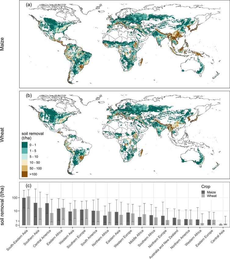
5264                                T. W. Carr et al.: Uncertainties, sensitivities and robustness of simulated water erosion

   Despite its importance for global agriculture, water ero-          Most global soil removal estimates using water erosion
sion is usually not considered in global gridded crop model        models are based on static observation approaches or on very
(GGCM) studies. Throughout the past decade, GGCMs –                coarse timescales that do not fall below annual time steps
typically combinations of agronomic or ecosystem models            (Borrelli et al., 2017). Therefore, seasonal patterns of soil
and global gridded input data infrastructures – have become        cover and precipitation intensities are neglected even though
essential tools for climate change impact assessments, evalu-      they are crucial factors for water erosion. The state of the soil
ations of agricultural externalities and as input data providers   and its cover is influenced by land management, such as the
for agro-economic models (Mueller et al., 2017). Few assess-       choice of crops, planting and harvest dates, tillage, and plant
ments have considered land degradation processes and found         residue management. Accordingly, neglecting the impact of
their inclusion and understanding crucial for evaluating cli-      seasonal changes in vegetation cover and field management
mate change mitigation and adaptation strategies (Balkovič        practices constitutes large uncertainty in global water erosion
et al., 2018; Chappell et al., 2016). Beyond crop models,          estimates. Crop models usually simulate crop growth on a
there is a need to improve the representation of agricultural      daily timescale, which allows attached water erosion models
management and soil-related processes in earth system mod-         to account for daily changes in weather, soil properties and
els to better reflect carbon sinks and sources (Luo et al.,        vegetation cover. However, uncertainty remains due to the
2016; McDermid et al., 2017; Pongratz et al., 2018). More-         increasing requirement of input data for daily simulations,
over, improving the representation of water erosion in large-      which is especially challenging at a global scale.
scale models is urgently needed to inform major environmen-           The overall aims of this study are (i) to analyse the
tal and agricultural policy programmes such as the European        robustness of water erosion estimates in all global agro-
Union’s Common Agricultural Policy (CAP), the United Na-           environmental regions simulated with an EPIC-based global
tions Sustainable Development Goals (SDGs), the United             gridded crop model and (ii) to discuss the main drivers affect-
Nations Convention to Combat Desertification (UNCCD)               ing the robustness and the uncertainty of simulated water ero-
and the Intergovernmental Science-Policy Platform on Bio-          sion rates on a global scale. We simulate global water erosion
diversity and Ecosystem Services (IPBES) (Alewell et al.,          rates in maize and wheat fields using different empirical ero-
2019). Yet, the necessary algorithms to simulate water ero-        sion equations in EPIC while accounting for the daily crop
sion are often not incorporated into such models. Exceptions       growth and development under different field management
among field-scale crop models, which are frequently used           scenarios. Here, maize and wheat are used as representative
in GGCM ensemble studies, are the Environmental Policy             crops of global agriculture, as they are grown under most en-
Integrated Climate model (EPIC) and Agricultural Produc-           vironmental conditions and represent contrasting soil cover
tion Systems Simulator (APSIM). Compared to other com-             patterns. Our global simulations are carried out for a baseline
monly used crop models in GGCMs, EPIC stands out in its            crop management scenario based on a set of environmental
detailed representation of soil processes including water ero-     and country-specific assumptions and indicators, which is a
sion and the impacts of tillage on soil properties (Folberth et    common practice in global gridded crop modelling. In addi-
al., 2019).                                                        tion, we quantify the uncertainties of simulated water erosion
   Recently, water erosion models such as the Universal Soil       values stemming from (i) uncertain field management inputs
Loss Equation (USLE) and the Revised Universal Soil Loss           and (ii) water erosion calculation methods. We also evaluate
Equation (RUSLE) have been used to estimate global wa-             the model’s sensitivity to all inputs involved in the water ero-
ter erosion. Annual global soil removal estimates and water        sion calculation to interpret the variability and uncertainties
erosion rates on cropland of recent studies range between          of the simulation results, as well as to discuss the differences
13 and 22 Gt and between 11 and 13 t ha−1 , respectively           between water erosion equations. Finally, we use field mea-
(Borrelli et al., 2017; Doetterl et al., 2012; van Oost et al.,    surements from various locations worldwide to evaluate the
2007). USLE and its modifications were developed in the            robustness of estimated water erosion rates under different
Midwestern United States and should ideally be evaluated           environmental conditions.
against soil erosion measurements when used for other agro-
environmental zones (Evans and Boardman, 2016). However,
the uneven distribution of field data around the world, the        2   Methods
lack of long-term soil measurements in most global regions
and the great variability of the designs of erosion rate mea-      The simplified framework in Fig. 1 illustrates the particular
surements hamper the evaluation of global soil loss estimates      stages of the methodological procedure applied by this study
derived from models (Auerswald et al., 2004; Borrelli et al.,      and their relationships to input data and model outputs. Both
2017; García-Ruiz et al., 2015). In addition, model input data     input and output data are used in two ways. We use input
on topography, soil properties and land use are often aggre-       data (i) to simulate daily maize growth, daily wheat growth
gated over large areas; thus, simulation results cannot be di-     and water erosion with EPIC and (ii) to analyse the sensi-
rectly compared to single field measurements at specific lo-       tivity of relevant model parameters to simulate global water
cations.                                                           erosion with all equations in EPIC. We use model outputs

Biogeosciences, 17, 5263–5283, 2020                                                   https://doi.org/10.5194/bg-17-5263-2020

T. W. Carr et al.: Uncertainties, sensitivities and robustness of simulated water erosion                                          5265

Figure 1. Scheme of the procedure used for simulating global water erosion with EPIC-IIASA and for analysing the uncertainty, sensitivity
and robustness of our simulation setup.

(i) to calculate a baseline global water erosion scenario and          These are aggregated to homogenous response units and fur-
(ii) to address the uncertainty of simulation results. The fi-         ther intersected with a 300 × 300 climate grid, the resolution
nal step of this study consists of the robustness check of the         at which global gridded climate data are available. This re-
model outputs using field data. A detailed description of each         sults in a total of 131 326 grid cells with a spatial resolution
element of this study is described in the following sections.          ranging between 50 and 300 (about 9 to 56 km near the Equa-
                                                                       tor) (Skalský et al., 2008). We use global daily weather data
2.1     Modelling water erosion and crop growth with                   from the AgMERRA dataset for the years 1980–2010 (Ruane
        EPIC                                                           et al., 2015), soil information from the Harmonized World
                                                                       Soil Database (FAO/IIASA/ISRIC/ISSCAS/JRC, 2009) and
2.1.1    Global gridded crop model and input data                      topography from USGS GTOPO30 (USGS, 1997). Each grid
                                                                       cell is represented by a single field characterized by the
We use a global gridded version of the Environmental Pol-              combination of topography and soil conditions prevailing
icy Integrated Climate (EPIC) crop model, EPIC-IIASA                   in this landscape unit. Each representative field has a de-
(Balkovič et al., 2014), to simulate soil sediment loss with          fined slope length (20–200 m) and field size (1–10 ha) based
runoff from 1980 to 2010 while accounting for the daily                on a set of rules for different slope classes (Table S1). The
growth of maize and wheat under different field manage-                slope of each representative field is determined by the slope
ment scenarios. EPIC can simulate the growth of a wide                 class covering the largest area in each grid cell (Table S1).
range of crops and has a sophisticated representation of car-          Slope classes are taken from a global terrain slope database
bon, nutrient and water dynamics as well as a wide variety             (IIASA/FAO, 2012) and are based on a high-resolution 90 m
of possible field management options, including tillage op-            Shuttle Radar Topography Mission (SRTM) digital elevation
erations and crop rotations (Izaurralde et al., 2006; Sharpley         model. In each grid cell, we consider reported growing sea-
and Williams, 1990). Originally, EPIC was named Erosion-               sons for maize and wheat (Sacks et al., 2010) and spatially
Productivity Impact Calculator and was developed to deter-             explicit nitrogen and phosphorus fertilizer application rates
mine the relationship between erosion and soil productiv-              (Mueller et al., 2012).
ity. Due to its origin, EPIC has several options to calculate
water erosion caused by precipitation, runoff and irrigation
(Williams, 1990).                                                      2.1.2   Water erosion equations
   EPIC-IIASA requires global soil and topography data and
daily weather data. The basic spatial resolution of the model          EPIC includes seven empirical equations to calculate water
is 50 × 50 at which soil and topographic data are provided.            erosion (Wischmeier and Smith, 1978). The basic equation

https://doi.org/10.5194/bg-17-5263-2020                                                        Biogeosciences, 17, 5263–5283, 2020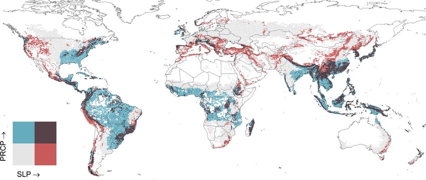
5266                                T. W. Carr et al.: Uncertainties, sensitivities and robustness of simulated water erosion

is                                                                 2.1.3    Field management scenarios

Y = R × K × LS × C × P ,                                    (1)    Field management techniques influencing soil properties and
                                                                   soil cover have a significant impact on the amount of wa-
where Y is soil erosion (t ha−1 ) (mass per area), R is the ero-   ter erosion. However, these methods are very heteroge-
sivity factor (erosivity unit per area), K is the soil erodibil-   nous around the world, and data on different field manage-
ity factor (t MJ−1 ) (mass per erosivity unit), LS is the slope    ment techniques are sparse. Therefore, three tillage manage-
length and steepness factor (dimensionless), C is the soil         ment scenarios – conventional tillage, reduced tillage and no
cover and management factor (dimensionless), and P is the          tillage – were designed by altering parameters related to wa-
conservation practices factor (dimensionless).                     ter erosion to analyse the impact of field management on sim-
   The main difference between the water erosion equations         ulated water erosion and to draw conclusions on its impact on
available in EPIC is their energy components used to calcu-        the quality of simulation results.
late the erosivity factor. The USLE, RUSLE and RUSLE2                  In the reduced and no-tillage scenarios, we decrease soil
equations (Table 1) use precipitation intensity as an ero-         disturbance by reducing cultivation operations, tillage depth
sive energy to calculate the detachment of soil particles. The     and surface roughness, and we increase plant residues left in
Modified Universal Soil Loss Equation (MUSLE) and its              the field after harvest. In addition, we reduce the runoff curve
variations MUST and MUSS use runoff variables to sim-              numbers, which indicate the runoff potential of a hydrolog-
ulate water erosion and sediment yield. The Onstad–Foster          ical soil group, land use and treatment class, with decreas-
equation (AOF) combines energy through rainfall and runoff         ing tillage intensification, by using pre-defined values for the
(Table 1).                                                         cover treatment classes presented in Table 2 (Sharpley and
   The erosion energy component is calculated as a function        Williams, 1990). By lowering the runoff curve numbers, the
of runoff volume Q (mm), peak runoff rate qp (mm h−1 ) and         impact of reduced tillage practices on the hydrologic balance
watershed area WSA (ha) or via the rainfall erosivity index        can be taken into account (Chung et al., 1999). We simulate
EI (MJ ha−1 ). The EI determines the detachment of soil par-       each tillage scenario with and without green fallow cover in
ticles through the energy of daily precipitation and a statisti-   between growing seasons, leading to a total of six field man-
cal estimate of the daily maximum intensity of precipitation       agement scenarios.
falling within 30 min. RUSLE2 is the only equation calcu-
lating soil deposition. If the sediment load exceeds the trans-    2.2     Baseline scenario for estimating global water
port capacity, determined by a function of flow rate and slope             erosion in wheat and maize fields
steepness, soil is deposited, which is calculated by a function
of flow rate and particle size (USDA-ARC, 2013).                   We estimate the rate of water erosion globally by combining
   The soil cover and management factor is updated for every       these six tillage and cover crop scenarios in different regions
day where runoff occurs using a function of crop residues,         of the world, using climatic and country-specific assump-
biomass cover and surface roughness. The impact of soil            tions and indicators (Table 3). We chose maize and wheat
erodibility on simulated water erosion is calculated for the       as two contrasting crop types for analysing water erosion in
topsoil layer at the start of each simulation year as a func-      different cultivation systems. Maize is a row crop with rel-
tion of sand, silt, clay and organic carbon content. The to-       atively large areas of bare and unprotected soil between the
pographic factor is calculated as a function of slope length       crop rows. The plant density in wheat fields is much higher,
and slope steepness. A detailed description of the cover and       which improves the protection of soils against water erosion.
management, soil erodibility, and topographic factor is pro-          We consider conventional and reduced tillage systems
vided in the Supplement (Sect. S1). The conservation prac-         globally while considering no tillage only for countries in
tice factor is included in all equations as a static coefficient   which the share of conservation agriculture is at least 5 %.
ranging between 0 and 1, where 0 represents conservation           In tropical regions, we simulate water erosion with a green
practices that prevent any erosion and 1 represents no conser-     cover in between maize and wheat seasons to account for
vation practices. Typical conservation practice factors can be     soil cover from a year-round growing season. In temperate
derived from tables, which include values ranging from 0.01        and snow regions, we simulate water erosion affected by both
to 0.35 for terracing strategies and from 0.25 to 0.9 for dif-     soil cover throughout the year and bare soil in winter seasons.
ferent contouring practices (Morgan, 2005; Wischmeier and          In arid regions, we do not simulate green cover in between
Smith, 1978). Alternatively, values can be derived from local      growing seasons due to the limited water supply.
field studies and remote sensing (Karydas et al., 2009; Pana-         On slopes steeper than 5 %, we consider only rainfed agri-
gos et al., 2015), from equations using topographical data         culture, as hilly cropland is irrigated predominantly on ter-
(Fu et al., 2005; Terranova et al., 2009) or from economic         races that prevent water runoff. To account for erosion con-
indicators (Scherer and Pfister, 2015).                            trol measures on steep slopes, we use a conservation P factor
                                                                   of 0.5 on slopes steeper than 16 %, and a P factor of 0.15 on
                                                                   slopes steeper than 30 % to simulate contouring and terracing

Biogeosciences, 17, 5263–5283, 2020                                                   https://doi.org/10.5194/bg-17-5263-2020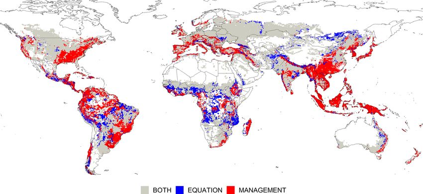
T. W. Carr et al.: Uncertainties, sensitivities and robustness of simulated water erosion                                        5267

Table 1. Equations for calculating the erosivity factor in each water erosion equation available in EPIC.

                  Erosivity factor                                 Equation
                  R = EI                                     (2)   USLE, RUSLE, RUSLE2 (Renard et al., 1997;
                                                                   USDA-ARC, 2013; Wischmeier and Smith, 1978)
                  R = 0.646 × EI + 0.45 × (Q × qp )0.33      (3)   AOF (Onstad and Foster, 1975)
                                      0.56
                  R = 1.586 × Q × qp        × WSA0.12        (4)   MUSLE (Williams, 1975)
                  R = 2.5 × Q × qp 0.5                       (5)   MUST (Williams, 1995)
                  R = 0.79 × (Q × qp )0.65 × WSA0.009        (6)   MUSS (Williams, 1995)

based on the range of P values presented by Morgan (2005).               be used to determine the impact of parameter interactions on
The threshold for slopes that are cultivated with conservation           the model output.
practices is based on the slope classes used for the under-                 We test 30 parameters directly connected to the water ero-
lying structure of slope information of EPIC-IIASA, from                 sion equations in EPIC. In total, we assign 126 976 random
which the three highest slope classes (16 %–30 %, 30 %–                  values to all input parameters along a pre-defined triangu-
45 %, >45 %) mark slopes that are less likely to be cultivated           lar distribution or a range of discrete values (Table S2). Wa-
without measures to prevent erosion. We choose the MUSS                  ter erosion is simulated with EPIC using the seven available
equation for the baseline scenario as it generates the lowest            equations for each random input combination at 40 locations
deviation between simulated and measured water erosion as                where wheat and maize are cultivated. To represent a het-
discussed below. Table 3 summarizes the field management                 erogenous distribution of global precipitation regimes, we
assumptions of the baseline scenario used to aggregate ero-              use the natural break optimization method to choose loca-
sion rates in each grid cell and region.                                 tions based on average annual precipitation amounts from
                                                                         1980 to 2010 (Jenks, 1967). For each location and equation,
2.3   Uncertainty analysis of field management scenarios                 the most sensitive parameters are ranked. To analyse the im-
      and water erosion equations                                        pact of precipitation regimes on the sensitivity of each pa-
                                                                         rameter, we use Spearman coefficients (ρ) to determine if
Given the global scale of the analysis and the aggregated                positive or negative relationships exist between each param-
nature of available field management information, there is               eter’s sensitivity and annual precipitation.
much uncertainty about crop management strategies, which
introduces uncertainty in the water erosion estimates. In ad-
                                                                         2.5    Evaluation of simulated erosion against reported
dition, each water erosion equation gives a different over-
                                                                                field measurements
all erosion estimate. To discuss the uncertainty of simulation
results, we evaluate the variance in simulated water erosion
rates at grid level due to (i) different management assump-              We compare our simulated water erosion rates with 606 soil
tions and (ii) the choice of water erosion equation. The vari-           erosion measurements on arable land from 36 countries rep-
ance of simulation outputs is defined as the range between               resenting plot and field scales. Most of the selected erosion
minimum and maximum simulated water erosion rates with                   rates are based on the 137 Cs method. In addition, data from
all combinations of tillage and cover crop scenarios and with            erosion plots and volumetric measurements of rills collected
each water erosion equation.                                             by Auerswald et al. (2009), Benaud et al. (2020) and García-
                                                                         Ruiz et al. (2015) are used. In total, 315 records are derived
2.4   Sensitivity analysis of model parameters                           by the 137 Cs method, 188 records from runoff plots and 103
                                                                         records from volumetric measurements of rills. An overview
We use a sensitivity analysis to identify the most essential             of the field data is presented in Fig. S4–S7, and the full
input parameters to the factors in the seven water erosion               dataset is available in Table S5.
equations. We use the Sobol method (Sobol, 1990), which                     Guidance on the 137 Cs method is provided by Fulajtar et
is a variance-based sensitivity analysis that is popular in              al. (2017), Mabit et al. (2014) and Zapata (2002). The 137 Cs
environmental modelling (Nossent et al., 2011). With this                radionuclide was released into the atmosphere by nuclear
method, it is possible to quantify the amount of variance that           weapon tests and from the accident of the Chernobyl Nu-
each parameter contributes to the total variance of the model            clear Power Plant and subsequently deposited in the upper-
output. These amounts are expressed as sensitivity indices,              most soil layer by atmospheric fallout. After its deposition,
which rank the importance of each input parameter for sim-               it was bound to soil colloids and can be moved only together
ulated water erosion. In addition, the sensitivity indices can           with soil particles by mechanical processes such as soil ero-

https://doi.org/10.5194/bg-17-5263-2020                                                           Biogeosciences, 17, 5263–5283, 2020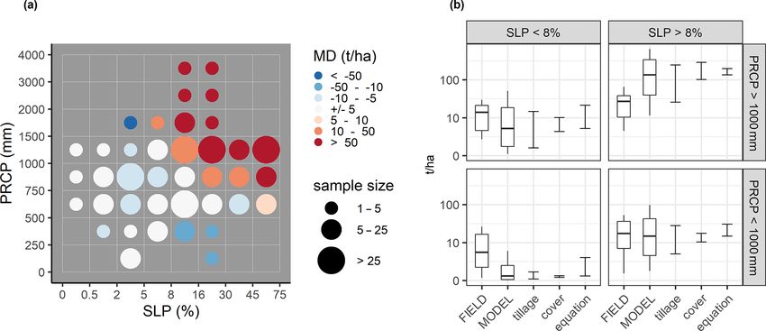
5268                                 T. W. Carr et al.: Uncertainties, sensitivities and robustness of simulated water erosion

Table 2. Tillage management scenarios for maize and wheat cultivation.

                                                     Conventional tillage   Reduced tillage    No tillage
                     Total cultivation operations    6–7                    4–5                3
                     Max surface roughness           30–50 mm               20 mm              10 mm
                     Max tillage depth               150 mm                 150 mm             40–60 mm
                     Plant residues left             25 %                   50 %               75 %
                     Cover treatment class           straight               contoured          contoured and terraced

Table 3. Management assumptions and erosion equation selected for the baseline scenario.

 Option                                      Baseline
 TILLAGE                                     – Mix of conventional, reduced and no tillage in regions where the national share of
                                             conservation agriculture is >5 % according to the latest reported data in
                                             AQUASTAT (2007–2014) (FAO, 2016): Argentina, Australia, Bolivia, Brazil, Canada, Chile,
                                             China, Colombia, Finland, Italy, Kazakhstan, New Zealand, Paraguay, Spain, USA, Uruguay,
                                             Venezuela, Zambia and Zimbabwe.
                                             – Mix of conventional and reduced tillage in the rest of the world.
 OFF-SEASON COVER                            – Cultivation only with cover crops in tropics according to Köppen–Geiger regions (Fig. S1)
                                             (Kottek et al., 2006). Mix of off-season cover with and without cover
                                             crops in temperate and cold zones.
                                             – No cover crops in arid regions.
 CONSERVATION PRACTICE FACTOR                Slope         0 %–16 %   16 %–30 %      >30 %
                                             P factor      1.0        0.5            0.15
 CROP                                        Water erosion is simulated in wheat and maize fields based on the global crop distribution
                                             by MIRCA2000 (Fig. S2) (Portmann et al., 2010).
 IRRIGATION                                  Only on slopes ≤ 5 %. Weighted average of irrigated and rainfed cropland based
                                             on MIRCA2000 (Portmann et al., 2010).
 METHOD                                      MUSS water erosion equation.
 AGGREGATION                                 Median of all management scenarios per grid cell and region.

sion. Its chemical mobility and uptake by plants is negligible           and Coshocton wheels). The overview of this method is pro-
(Mabit et al., 2014; Zapata, 2002). If part of the topsoil con-          vided by Cerdan et al. (2010); Hudson (1993); Mutchler et
taminated by 137 Cs is removed by erosion, the 137 Cs concen-            al. (1994); De Ploey and Gabriels (1980); and Zachar (1982).
trations in soil profiles can be used to trace soil movements               The volumetric measurements of rill erosion were used
using the mass balance equation (Walling et al., 2014). A                since approximately the 1940s in the USA (Kaiser, 1978,
major advantage of the 137 Cs method is that it provides long-           in Evans, 2013) and the 1950s in Europe (Lobotka, 1955),
term mean erosion rates (representing the period since 137 Cs            usually at the field scale (Boardman, 1990, 2003; Boardman
fallout in the 1960s until the time of sampling) and over-               and Evans, 2020; Brazier, 2004; Evans, 2002, 2013; Herweg,
comes the problem of high temporal variability of erosion.               1988; Zachar, 1982). The volume of erosion rills is derived
   Bounded plots are the most commonly used method of                    from their lengths and profile cross-section areas, which are
erosion measurements. They were introduced in the USA                    measured in field or from terrestrial and aerial photos (Evans,
in the 1920s (Hudson, 1993) and were used for the devel-                 1986; Watson and Evans, 1991).
opment of the USLE and WEPP models (Brazier, 2004).                         The overwhelming effect of the experimental methodol-
Eroded soil material can be quantified with erosion plots in             ogy on measured erosion rates, the lack of sufficient metadata
different ways (total collection of sediment, fractioned col-            accompanying erosion measurements and the granular spa-
lection of sediments using multislot divisors, measurement               tial resolution of our simulation setup hinders a direct com-
of discharge and sediment concentration by tipping buckets               parison between simulated and observed water erosion rates.

Biogeosciences, 17, 5263–5283, 2020                                                           https://doi.org/10.5194/bg-17-5263-2020
T. W. Carr et al.: Uncertainties, sensitivities and robustness of simulated water erosion 5269
Instead we compare aggregated simulated and observed ero- sion rates are simulated with management scenarios includ-
sion values for different slope and precipitation classes to ing no tillage and cover crops. For 86 % of grid cells, max-
analyse the robustness of simulated water erosion rates un- imum erosion rates are simulated under conventional tillage
der different environmental conditions. Therefore, only mea- without cover crops. The annual median uncertainty range
surements with recorded slope steepness and annual precip- at each grid cell due to the choice of erosion equation is
itation are used. Where annual precipitation is not recorded, 23 t ha−1 . In 74 % of grid cells, the lowest erosion rates are
it is taken from the WorldClim2 dataset (Fick and Hijmans, simulated with the MUSS equation. The highest erosion val-
2017). Due to the non-normal distribution of the simulated ues are simulated with RUSLE (46 %), followed by USLE
and measured data, the median deviation (MD) is used as a (25 %).
measure to compare the agreement between simulated and In most locations, the uncertainty due to field management
measured water erosion values. exceeds the uncertainty caused by choice of erosion equa-
tion. For 46 % of grid cells, management scenarios cause the
prevailing uncertainty, which we defined as the higher uncer-
3 Results tainty range by at least 5 t ha−1 . The selected erosion equa-
tion causes higher uncertainty by at least 5 t ha−1 in 14 % of
We estimate global median water erosion rates of 7 and grid cells. The map in Fig. 4 illustrates the global distribution
5 t ha−1 in maize and wheat fields, respectively. The total re- of prevailing uncertainty sources.
moval of soil in global maize and wheat fields is estimated to
be 5.3 and 1.9 Gt a−1 , respectively. The map in Fig. 2 illus- 3.2 Main drivers of the global erosion model
trates the global distribution of simulated water erosion rates.
Highest water erosion is simulated in mountainous regions We designed the sensitivity study to explain the large vari-
and regions with strong precipitation, especially in tropical ability of simulated water erosion rates in different regions
climate zones. In Asia, those regions are widespread in the and to discuss the main differences between water erosion
east, south-east and the Himalaya region. In Africa, simi- equations. Water erosion is highly sensitive to slope steep-
lar areas with high water erosion values are spread around ness (SLP) for all equations. The first-order sensitivity index
the continent and are most common at the west coast and in of the slope parameter indicates that 46 %–54 % of the vari-
East Africa, including broad areas in Guinea, Sierra Leone, ance in the model output is attributable to the slope, without
Liberia, Ethiopia and Madagascar. In South America, high- considering interactions between the input parameters (Ta-
est water erosion is simulated in the south of Brazil and re- ble 4). Daily precipitation (PRCP) is the second most impor-
gions around the Andes mountain range and the Amazon tant parameter for calculating water erosion, with an individ-
river basin. The highest water erosion values on the Amer- ual contribution of around 9 %–20 % to the variance of the
ican continent are simulated in tropical Central America and output. The remaining parameters contribute together 4 %–
the Caribbean. In North America, highest water erosion oc- 13 % to the output variance.
curs along the west coast and in the east. Water erosion in Eu- The first-order sensitivity indices do not include interac-
rope is highest in Mediterranean areas and around the Alps. tions between input parameters, which leads to the sum of all
Median annual water erosion values for the five largest first-order sensitivity indices being lower than 1. The total-
wheat- and maize-producing countries demonstrate the order sensitivity indices sum all first-order effects and inter-
strong impact of climate and topography on simulated wa- actions between parameters, which leads to overlaps in the
ter erosion. In Brazil, China and India, where a large pro- case of interactions and a sum greater than 1. The differences
portion of cropland is in tropical areas, water erosion is rela- between the first-order and the total-order indices can be used
tively high with annual median values of 10, 6 and 37 t ha−1 , as a measure to determine the impact of the interactions be-
respectively. In Russia and the United States, annual me- tween a specific parameter with other parameters. The total-
dian values are much lower with 1 and 2 t ha−1 , respectively. order sensitivity indices show that slope steepness, including
Overall, Fig. 2 illustrates the large variation in simulated wa- interactions to other parameters, contributes 63 %–75 % of
ter erosion between tropical climate regions and regions with the output variance from which 18 %–21 % is due to interac-
a large proportion of flat and dry land. tive effects with other parameters (Table 5). The total-order
sensitivity indices from precipitation range from 21 %–36 %,
3.1 Sources of model uncertainty related to from which 10 %–18 % is due to interactions with other pa-
management assumptions and method selection rameters.
The high sensitivity of slope and precipitation is simi-
The uncertainty of the simulation results due to management lar for all equations, but the most sensitive parameters after
scenarios and the choice of water erosion equations is high- these can be different for each equation. Equations estimat-
est in regions most vulnerable to water erosion (Fig. 3). The ing erosion energy by surface runoff and the RUSLE2 equa-
annual median uncertainty range at each grid cell due to man- tion are very sensitive to the hydrological soil group (HSG),
agement is 30 t ha−1 . For 97 % of grid cells, the lowest ero- which determines the soils infiltration ability. This parameter
https://doi.org/10.5194/bg-17-5263-2020 Biogeosciences, 17, 5263–5283, 20205270 T. W. Carr et al.: Uncertainties, sensitivities and robustness of simulated water erosion Figure 2. Soil loss due to water erosion in maize (a) and wheat (b) fields simulated with the baseline scenario. Each pixel cell illustrates the median relative water erosion of one representative field. The extent of cropland areas is not considered in pixel cell size. The bars in the bottom plot (c) illustrate median soil removal for major world regions simulated under maize and wheat cultivation. The lines and whiskers illustrate the 25th and 75th percentile values. The classification of world regions is illustrated in Fig. S3. Due to the large gap between aggregated values, all values in the bottom plot have been log-transformed to facilitate the visual comparison. is used in the calculation of the curve number, which defines evant for field management, such as surface roughness and the partition of precipitation into runoff and infiltration. Also, mixing efficiency of the topsoil, have little influence on wa- the land-use number (LUN), which is ranked among the most ter erosion. sensitive input parameters, is used for the calculation of the The sensitivity of slope steepness has a strong positive curve number. The most sensitive parameters of USLE and correlation with the amount of annual precipitation at each RUSLE, following slope inclination and daily precipitation, location (ρ = 0.69, p
T. W. Carr et al.: Uncertainties, sensitivities and robustness of simulated water erosion                                        5271

Figure 3. Water erosion uncertainty due to (a) field management assumptions and (b) water erosion equations.

Figure 4. Prevailing uncertainty, defined as the higher uncertainty range by at least 5 t ha−1 .

https://doi.org/10.5194/bg-17-5263-2020                                                            Biogeosciences, 17, 5263–5283, 2020
5272                                  T. W. Carr et al.: Uncertainties, sensitivities and robustness of simulated water erosion

Table 4. First-order sensitivity indices (denoted SI) ranking for the five most sensitive input parameters (PARM) for each water erosion
equation including slope steepness (SLP), daily precipitation (PRCP), soil hydrologic group (HSG), land-use number (LUN), soil silt content
(SILT), soil sand content (SAND), curve number parameter (S301), maximum air temperature (TMX) and crop residues left after harvest
(ORHI). The sensitivity indices of the remaining parameters are presented in Table S3.

      Rank        AOF            MUSLE              MUSS              MUST             RUSLE2            RUSLE              USLE
             PARM        SI    PARM        SI   PARM        SI    PARM        SI    PARM        SI    PARM        SI    PARM        SI
      1.     SLP        0.47   SLP      0.47    SLP       0.46    SLP       0.48    SLP       0.46    SLP       0.50    SLP       0.54
      2.     PRCP       0.13   PRCP     0.10    PRCP      0.12    PRCP      0.09    PRCP      0.16    PRCP      0.20    PRCP      0.18
      3.     HSG        0.03   HSG      0.04    HSG       0.05    HSG       0.04    HSG       0.03    SAND      0.05    SILT      0.02
      4.     SILT       0.02   LUN      0.02    LUN       0.02    LUN       0.02    SAND      0.01    TMX       0.01    TMX       0.01
      5.     LUN        0.01   SILT     0.02    S301      0.01    SILT      0.02    LUN       0.01    ORHI      0.01    ORHI      0.01
      ...    ...         ...   ...       ...    ...        ...    ...        ...    ...        ...    ...        ...    ...        ...
      Sum               0.69            0.68              0.71              0.69              0.71              0.78              0.77

Table 5. Total-order sensitivity indices (denoted SI) ranking for the five most sensitive input parameters (PARM) for each water erosion
equation including slope steepness (SLP), daily precipitation (PRCP), soil hydrologic group (HSG), land-use number (LUN), soil silt content
(SILT), soil sand content (SAND), maximum air temperature (TMX) and crop residues left after harvest (ORHI). The sensitivity indices of
the remaining parameters are presented in Table S3.

      Rank        AOF            MUSLE              MUSS              MUST             RUSLE2            RUSLE              USLE
             PARM        SI    PARM        SI   PARM        SI    PARM        SI    PARM        SI    PARM        SI    PARM        SI
      1.     SLP        0.68   SLP      0.68    SLP       0.63    SLP       0.68    SLP       0.66    SLP       0.69    SLP       0.75
      2.     PRCP       0.28   PRCP     0.23    PRCP      0.22    PRCP      0.21    PRCP      0.32    PRCP      0.36    PRCP      0.36
      3.     HSG        0.09   HSG      0.12    HSG       0.13    HSG       0.12    HSG       0.08    SAND      0.12    SILT      0.05
      4.     SILT       0.07   LUN      0.07    LUN       0.07    LUN       0.07    LUN       0.05    TMX       0.02    TMX       0.02
      5.     LUN        0.05   SILT     0.07    SILT      0.05    SILT      0.07    SAND      0.04    ORHI      0.01    SAND      0.01
      ...    ...         ...   ...       ...    ...        ...    ...        ...    ...        ...    ...        ...    ...        ...
      Sum               1.29            1.30              1.25              1.27              1.34              1.27              1.27

are negatively correlated to annual precipitation with a mod-           recorded slope inclinations and annual precipitation amounts
erate strength (ρ = 0.45, p
T. W. Carr et al.: Uncertainties, sensitivities and robustness of simulated water erosion 5273 Figure 5. First-order and total-order sensitivity indices (SIs) for (a) slope steepness (%) and (b) precipitation (mm). The dashed vertical line illustrates median annual precipitation at all tested locations (1248 mm). Figure 6. Comparison of simulated erosion with measured erosion. (a) Median deviation (MD) (t ha1 ) between simulated erosion using the baseline scenario and measured erosion. Simulated and measured data are grouped into precipitation classes and slope classes used for the simulation setup. (b) Distributions of measured erosion rates, erosion rates simulated with the baseline scenario and uncertainty ranges for management assumptions and erosion equations. The boxplots are defined by the median, the 25th percentile and the 75th percentile of simulated and measured erosion rates. Whiskers illustrate the 10th and 90th percentiles. The three bars next to the boxplots illustrate minimum and maximum median erosion rates calculated with all tillage and cover crop scenarios and with all water erosion equations. The values have been log-transformed for better visualization. also be observed between the range of simulated and mea- range of simulated medians due to contrasting tillage man- sured water erosion values. Outside locations combining agement scenarios, cover crop scenarios and different wa- steep slopes and strong precipitation, median deviation be- ter erosion equations. At locations with low to moderate tween simulated and measured data is lower than the vari- slope steepness and annual precipitation, the measured water ability within the field data. The range of values at locations erosion values agree best with the simulation values gener- with lower precipitation and slope steepness demonstrates ated under scenarios implying larger water erosion, such as that simulated values are mostly below measured values in high-intensity tillage and low soil cover. On the other hand, those environments. at locations with steep slopes and intensive precipitation, The uncertainty in the choice of management scenarios the measured values are closer to the simulated values un- and water erosion equations included in our baseline scenario der scenarios with less-intensive tillage and more soil cover. leads to an uncertainty of the deviation between simulated In addition, the varying sensitivities of each water erosion and measured erosion values. This uncertainty is demon- equation lead to a different magnitude of water erosion val- strated in Fig. 6b by additional three bars illustrating the ues in different environments. On low-to-moderate slopes, https://doi.org/10.5194/bg-17-5263-2020 Biogeosciences, 17, 5263–5283, 2020
5274                                T. W. Carr et al.: Uncertainties, sensitivities and robustness of simulated water erosion

water erosion simulated with the MUSS equation is low-             for without calibration and model adaptation (e.g. Cohen et
est, whereas RUSLE generates the highest values. On steep          al., 2005; Labrière et al., 2015).
slopes, RUSLE generates the lowest water erosion values,              The skewed distribution of simulated water erosion values
which agree best with the measured values. The options to          influenced by extreme soil loss rates in few fields highly sen-
increase and decrease simulated water erosion with differ-         sitive to water erosion results in a large difference between
ent field management scenarios and water erosion equations         the global median value of 6 t ha−1 a−1 and the global aver-
creates both uncertainty in the model results but also the pos-    age value of 19 t ha−1 a−1 (Fig. S9). Due to the strong influ-
sibility to closely match field data.                              ence of outliers on average values, we used median values
   At locations combining steep slopes and intense precipi-        to represent global and regional water erosion rates in wheat
tation, most management scenarios and equations generate           and maize fields. The high sensitivity of the simulation re-
water erosion values that are higher than the measured val-        sults to slope inclinations and precipitation suggests that a
ues. However, those environmental conditions cover only            significant share of the estimated soil removal of 7.2 Gt a−1
a small share of global cropland. Cultivation areas with           originates from small wheat and maize cultivation areas on
slopes steeper than 8 % and annual precipitation higher than       steep slopes with strong annual precipitation.
1000 mm represent only 7 % of global maize and wheat crop-
land in our grid cells. The map in Fig. 7 illustrates that the     4.2     Sources of uncertainties in global water erosion
highest concentration of these areas is in East Asia and South             estimates
East Asia, followed by Central America, South America and
sub-Saharan Africa.                                                4.2.1    Uncertain land use in mountainous regions

                                                                   Changing climatic conditions with increasing elevation and
                                                                   the variable soils in mountainous regions can favour crop cul-
4     Discussion                                                   tivation in higher elevations over lower elevations (Romeo
                                                                   et al., 2015). However, upland farming without soil con-
4.1    Varying robustness of simulated water erosion in            servation measures can lead to exhaustive soil erosion and
       different global regions                                    can become a critical problem for agriculture (Montgomery,
                                                                   2007). Large areas of land have been abandoned due to high
Global water erosion estimates generated with an EPIC-             erosion rates as soils were no longer able to support crops
based GGCM and our baseline scenario overlap with ob-              (Fig. 8) (Romeo et al., 2015). As mountain agriculture is de-
served water erosion values under most of the climatic and         termined by various environmental and socioeconomic fac-
topographic environments where maize and wheat are grown.          tors, the cultivation of steep slopes can be very variable be-
However, global maize and wheat land include locations             tween regions. Regional erosion assessments in mountain-
where environmental characteristics differ significantly from      ous cropland suggested that areas with extreme water ero-
the Midwestern United States, where the data were collected        sion rates are mainly limited to marginal steep land cultivated
to develop the water erosion equations embedded in EPIC.           by smallholders (Haile and Fetene, 2012; Long et al., 2006;
The USLE model and its modification were developed with            Nyssen et al., 2019). In some mountainous regions, efforts to
data for slopes of up to 20 %, which makes model appli-            remove marginal farmlands from agricultural production and
cation for steeper slopes uncertain (McCool et al., 1989;          programmes to improve land management on steep slopes
Meyer, 1984). Furthermore, the relations between kinetic en-       have reduced high water erosion rates (Deng et al., 2012;
ergy and rainfall energy in the American Great Plains differ       Nyssen et al., 2015). On the contrary, recent pressure through
from other regions in the world (Roose, 1996). Similarly, the      increasing population and crop production demands has re-
runoff curve number method, which is the key methodology           sulted in recultivation of hillslopes and a reduction of fallow
for the calculation of surface runoff, is based on an empir-       periods, which limits the recovery of eroded soil (Turkel-
ical analysis in watersheds located in the United States and       boom et al., 2008; Valentin et al., 2008).
might be less reliable in different regions of the world (Ralli-      To analyse the sustainability of simulated maize and wheat
son, 1980). Due to the high sensitivity of slope steepness and     cultivation systems exposed to high erosion rates, we com-
daily precipitation for the calculation of water erosion, the      pare simulated annual eroded soil depth with a global dataset
reliability of the tested equations decreases in regions where     on modelled sedimentary deposit thickness (Pelletier et al.,
typical slope and precipitation patterns differ from the Mid-      2016). The comparison shows that at 4 % of grid cells perma-
western US. Although some studies have successfully used           nent maize and wheat cultivation would not be sustainable as
USLE and its modification under a different environmental          the whole soil profile would be eroded at the end of the sim-
context (e.g. Alewell et al., 2019; Almas and Jamal, 2009;         ulation period (Fig. S18). Most of the unsustainable agricul-
Fischer et al., 2018; Sadeghi and Mizuyama, 2007), many            ture is simulated on steep slopes. Although we account for
studies have concluded that the accuracy of these models           conservation techniques and cover crops, we do not imitate
may be reduced outside the environments they were created          the highly complex farming practices involving intercrop-

Biogeosciences, 17, 5263–5283, 2020                                                   https://doi.org/10.5194/bg-17-5263-2020
T. W. Carr et al.: Uncertainties, sensitivities and robustness of simulated water erosion 5275 Figure 7. Distribution of low-to-high slope steepness (SLP) and annual precipitation (PRCP) in maize and wheat fields. Dark areas illustrate grid cells where dominant slopes are steeper than 8 % and annual precipitation is above 1000 mm. Correspondingly, blue, red and grey pixels are below one or both thresholds. Figure 8. (a) Sugar cane cultivation on steep slopes in southern China (Nanning, Guangxi Zhuang Autonomous Region). The steepest slopes are already abandoned and reforested by eucalyptus trees. (b) Maize cultivation on strongly eroded slopes (30 %–60 %) in south-west Uganda (Kigwa, Kabale District). (c) Abandoned fields and maize cultivation on a steep slope (30 %–60 %) in south-west Uganda (Kigwa, Kabale District). (d) Degraded and abandoned maize fields on steep slopes (20 %–60 %) in northern El Salvador (San Ignacio, Chalatenango Department). The photos and additional examples are provided in Figs. S10–S17. https://doi.org/10.5194/bg-17-5263-2020 Biogeosciences, 17, 5263–5283, 2020
5276                                T. W. Carr et al.: Uncertainties, sensitivities and robustness of simulated water erosion

ping techniques and fallow periods, which are common on            this management strategy is likely according to AQUASTAT
hillslopes typically managed by smallholders (Turkelboom           (FAO, 2016). Furthermore, by assuming cover crops in be-
et al., 2008). Moreover, we assume that the slope class rep-       tween wheat and maize seasons we simulated more complex
resenting the largest area in each grid cell most likely rep-      cropping systems in the tropics, where long and year-round
resents the largest share of arable land. This builds on the       growing seasons and frequent multi-cropping farm practices
idea that a spatially extensive and diverse landscape can be       barely leave the soil uncovered. Hence, we did not simulate
represented by a single “representative field” characterized       bare fallow in the tropics as erroneously high water erosion
by the prevailing topography and soil conditions found in the      values would have been simulated at locations with heavy
landscape. On hilly terrain this setup simulates maize and         precipitation falling on bare soil. In addition, conservation
wheat cultivation on steep slopes and thus mainly represents       practices such as contouring and terracing are crucial to re-
unsustainable agriculture. Although unsustainable maize and        duce the simulation of high water erosion values on steep
wheat cultivation can be observed in several mountain re-          slopes. We simulated these practices for specific slope classes
gions, cropland is very heterogeneously distributed in moun-       under the assumption that farmers around the world uni-
tains and thus erosion rates from one representative field are     formly use conservation practices when cultivating on steep
highly uncertain.                                                  slopes. The most relevant parameters used for tillage scenar-
   The uncertainty in cropland distribution can partly be re-      ios are related to crop residues left in the field. In addition,
duced by developing a higher-resolution global gridded data        equations directly connected to surface runoff are strongly
infrastructure, which is currently not available for EPIC-         influenced by the land-use number used to determine the im-
IIASA. However, due to the large uncertainty in global land        pact of cover type and treatment on soil permeability. While
cover maps (Fritz et al., 2015; Lesiv et al., 2019), an ex-        both crop residues and green fallow decrease water erosion
plicit spatial link between cropland distribution and the cor-     significantly, especially in the tropics, their use varies widely
responding slope category cannot be established without on-        between regions and even farms, based on a complex web
site observations. We test the impact of this uncertainty for      of factors such as institutional factors, farm sizes, risk atti-
erosion estimates in Italy, where large maize and wheat cul-       tudes, interest rates, access to markets, farming systems, re-
tivation areas are distributed on both flat terrain in the north   source endowments and farm management skills (Pannell et
and mountainous regions in the south. In an ideal scenario         al., 2014). Also, soil conservation measures such as terraces
where cropland is limited to flattest land available per grid      or contour farming significantly influence water erosion but
cell, median simulated water erosion in Italy would be re-         are very heterogeneously used between regions, farming sys-
duced to tolerable levels below 1 t ha−1 . However, in a sce-      tems and farmers. Our baseline scenario is a very rough de-
nario where the most common slopes per grid cell are culti-        piction of the complex patterns of field management around
vated, median simulated water erosion increases to 14 t ha−1       the world but attempts to represent these highly influential
due to high water erosion simulated in Italy’s mountainous         practices with the limited available data.
regions (Fig. S19). This suggests a high uncertainty in global
water erosion estimates due to uncertain spatial links be-         4.2.3   Variable estimates from different water erosion
tween maize and wheat cultivation areas and different slope                equations
categories.
                                                                   The water erosion equation chosen for the baseline scenario
4.2.2   Uncertain field management                                 generates the lowest global soil removal estimate. Different
                                                                   water erosion equations embedded in EPIC estimate a higher
Simulated water erosion values are highly variable depend-         global soil removal of up to 11 Gt a−1 as well as higher me-
ing on the field management scenario. Simulating cover             dian water erosion rates up to 19 t ha−1 a−1 . The MUSS wa-
crop and no tillage worldwide results in the lowest global         ter erosion equation chosen for the baseline scenario gener-
soil removal of 2 Gt a−1 with median water erosion rates of        ates water erosion rates closest to the field data. The focus
1 t ha−1 a−1 and simulating no cover crops and conventional        of equations on either rainfall energy or runoff energy is rel-
tillage worldwide results in the highest global soil removal of    evant for the different simulation results under specific en-
13 Gt a−1 with median water erosion rates of 17 t ha−1 a−1 .       vironmental conditions. Equations based on rainfall energy
These variations cause further uncertainties in the simulation     such as RUSLE and USLE simulate higher water erosion val-
results.                                                           ues than the other equations at most locations. However, on
    Indeed, a proper reconstruction of a business-as-usual field   steep slopes they generate the lowest water erosion values
management is important to further narrow down the un-             as runoff becomes a greater source of energy than rain with
certainty in global crop modelling (Folberth et al., 2019).        increasing slope steepness (Roose, 1996). Also, the vary-
In this study we allocated prevailing field management us-         ing sensitivities of other parameters to the equations such as
ing a set of environmental- and country-specific indicators,       soil properties and management parameters lead to a varying
similarly to Porwollik et al. (2019). For example, we ac-          agreement between simulated data and field data depending
counted for conservation agriculture only in countries where       on the equation selection. Detailed field data would facili-

Biogeosciences, 17, 5263–5283, 2020                                                   https://doi.org/10.5194/bg-17-5263-2020
T. W. Carr et al.: Uncertainties, sensitivities and robustness of simulated water erosion 5277
tate the choice of an appropriate equation to simulate water data derived from erosion plots, field-scale measurements,
erosion worldwide or for a specific region. catchment-scale measurements using hydrological methods,
137 Cs-method, soil profile truncation and elevated cemetery
4.3 The difficulty of evaluating large-scale erosion plots.
estimates with field data Whilst all erosion measurement methods are open to criti-
cism, we decided to use only data obtained by field measure-
The selection of field data for evaluating simulated water ero- ments from runoff plots, by the 137 Cs method and volumetric
sion was limited by the low availability of suitable water ero- surveys as these methods are most suitable at plot, slope and
sion observations covering the entire globe. The lack of reli- field scales. Geodetic methods such as erosion pins and laser
able data on water erosion rates is a severe obstacle for un- scanner are also used at plot to field scales, but their accuracy
derstanding erosion, developing and validating models, and is much lower than the accuracy of plot measurements and
implementing soil conservation (Boardman, 2006; Nearing the 137 Cs method. Furthermore, erosion pins are mainly suit-
et al., 2000; Poesen et al., 2003; Trimble and Crosson, 2000). able for areas with extreme erosion rates (Hsieh et al., 2009;
The main reasons for the low availability of suitable data to Hudson, 1993), and laser scanners have difficulties to recog-
evaluate simulated water erosion rates are twofold: (i) ero- nize vegetation (Hsieh et al., 2009). Other commonly used
sion monitoring is expensive, time consuming and labour methods such as the hydrological method (measurements of
demanding; (ii) primary data and metadata of measurement discharge and suspended sediment load) and the bathymet-
sites accompanying final results are often not available, and ric method are more suitable for larger scales and involve a
many older measurements are poorly accessible as they are significant portion of channel erosion, which is not related to
not available online (Benaud et al., 2020). A variety of fac- agricultural land (García-Ruiz et al., 2015). We did not con-
tors influencing water erosion such as climate, field topogra- sider plot experiments using rainfall simulators as they are
phy, soil properties and field management need to be consid- usually performed on small plots with artificially generated
ered when modelling water erosion but are often not reported rainfall, which mostly have very low energies and thus gen-
in available field measurements (García-Ruiz et al., 2015). erate low erosion rates (Boix-Fayos et al., 2006; García-Ruiz
This hampers a direct comparison between simulated and et al., 2015).
observed water erosion values. We demonstrated the vary- The 137 Cs method was criticized by Parsons and Fos-
ing match between measured and simulated water erosion ter (2013), who questioned assumptions about the 137 Cs
using different tillage and cover crop scenarios. Metadata on behaviour in the environment (variability of the 137 Cs in-
field management often only provides the crop cultivated and put by wet fallout, its micro-spatial variability at reference
therefore the conditions under which erosion was measured sites, its possible mobility in certain soils, the 137 Cs uptake
in the field are not known sufficiently to evaluate erosion val- by plants and other aspects of 137 Cs behaviour in soil). To
ues simulated under different field management scenarios. confront the criticism against the 137 Cs method, Mabit et
Similarly, information on field topography and soil proper- al. (2013) discussed all objections raised by Parsons and Fos-
ties is often not provided with recorded field measurements; ter (2013) and confirmed its accuracy by listing several stud-
thus, their use is limited in an evaluation of water erosion ies, in which 137 Cs-based erosion rates are compared with
estimates simulated in different global environments. More- erosion rates derived from direct measurements. The 137 Cs
over, most data are concentrated in the United States, western method is based on a set of presumptions which should be
Europe and the western Mediterranean (García-Ruiz et al., met to produce useful results and thus careful interpretation
2015). In summary, there is a lack of field data representing of the obtained results is needed (Fulajtar et al., 2017; Mabit
all needed regions, situations and scenarios (Alewell et al., et al., 2014; Zapata, 2002).
2019). Similarly, erosion rates obtained by volumetric measure-
The appropriate selection of field data to evaluate model ments require careful interpretation as they are exposed to
outputs needs to be considered as well. At different spa- various potential sources of errors and do not account for
tial scales different erosion processes are dominant and con- inter-rill erosion. Although the latter can be neglected un-
sequently different erosion measurement methods are suit- der certain circumstances, studies from Europe and semiarid
able (Boix-Fayos et al., 2006; Stroosnijder, 2005). Most au- areas of the USA have reported that inter-rill erosion con-
thors use very heterogeneous datasets to evaluate their mod- tributed significantly to the amount of soil eroded in fields
els, involving data generated by different methods at vari- (Boardman and Evans, 2020; Parsons, 2019). Further, mea-
able time and spatial scales and variable quality. For exam- suring the lengths and cross sections of rills during field sur-
ple, Doetterl et al. (2012) used plot data, suspended sed- veys or on terrestrial and aerial photos can be very subjective
iments from rivers data from RUSLE modelling. Borrelli (Panagos et al., 2016). Different approaches used to detect
et al. (2017) used soil erosion rates (measurement methods and measure rills in fields can cause variability in calculated
are not specified), remote sensing, vegetation index (NDVI) erosion volumes up to a factor of 2 (Boardman and Evans,
and results of RUSLE modelling. In his review on erosion 2020; Casali et al., 2006; Watson and Evans, 1991). In order
rates under different land use, Montgomery (2007) used field to obtain soil erosion rates in weight units, soil volumes need
https://doi.org/10.5194/bg-17-5263-2020 Biogeosciences, 17, 5263–5283, 2020You can also read


