A non reflecting wave equation through directional wave field suppression and its finite difference implementation - Nature
←
→
Page content transcription
If your browser does not render page correctly, please read the page content below

www.nature.com/scientificreports
OPEN A non‑reflecting wave equation
through directional wave‑field
suppression and its finite difference
implementation
Teun Schaeken, Leo Hoogerbrugge* & Eric Verschuur
The acoustic wave equation describes wave propagation directly from basic physical laws, even in
heterogeneous acoustic media. When numerically simulating waves with the wave equation, contrasts
in the medium parameters automatically generate all scattering effects. For some applications -
such as propagation analysis or certain wave-equation based imaging techniques - it is desirable
to suppress these reflections, as we are only interested in the transmitted wave-field. To achieve
this, a modification to the constitutive relations is proposed, yielding an extra term that suppresses
waves with reference to a preferred direction. The scale-factor α of this extra term can either be
interpreted as a penetration depth or as a typical decay time. This modified theory is implemented
using a staggered-grid, time-domain finite difference scheme, where the acoustic Poynting-vector is
used to estimate the local propagation direction of the wave-field. The method was successfully used
to suppress reflections in media with bone tissue (medical ultrasound) and geophysical subsurface
structures, while introducing only minor perturbations to the transmitted wave-field and a small
increase in computation time.
Numerical simulations of propagating wave-fields in complex heterogeneous media play an essential role in the
field of acoustical imaging. Through a combination of acoustic recordings and numerical wave equation simu-
lations, images of physically inaccessible, vastly differently sized objects can be made. Despite their numerical
nature, these simulations honour the physical laws of wave theory.
One of these acoustical imaging methods is known as reverse time migration (RTM)1,2. RTM is comprised
of two modeling phases, a forward modeling of source data and a backward modeling of time-reversed receiver
data. In its most basic form, RTM creates an image through a cross-correlation of forward modeled shot data
and backward modeled, time-reversed, receiver data. In the past, this modeling phase was often performed using
one-way propagators3,4. Nowadays, due to the increasing advances in computational processing and storage
capabilities, finite difference modeling (FD) of the complete, two-way wave equation has become the preferred
approach. A common problem in prestack-RTM is the formation of image artifacts due to the cross-correlation
of unwanted reflections. These artifacts can be avoided directly, by suppressing these reflections within the
simulation5, or indirectly, by means of angle-gathers6,7.
Recently, RTM, which has been developed for geophysical imaging, has also found its way to ultrasound
applications like civil engineering8,9 and photo-acoustic imaging10. In medical applications, RTM has also shown
to be successful in imaging breast-tissue using frequency domain finite difference modeling (FDFD)11,12. Other
geophysical imaging methods, such as Full Waveform Inversion (FWI)13, have also been successfully applied
to medical ultrasound imaging of high-contrast bone tissue, such as the human s kull14. For these methods, dis-
tinguishing complex back-scattering from multiple arrivals by means of reflection suppression could serve as a
useful tool within wave propagation analysis.
An obvious method to remove reflections is to smooth the inverse of the wave-speed (slowness) of the
medium. This approach, however, is less effective for high-frequency components of the wave-field and comes
at the expense of inaccurate wave propagation. Another popular method, matching the impedance inside the
medium15, is only effective in suppressing reflections at small angles of incidence and does not preserve the origi-
nal wave amplitudes. A final alternative is an approach where reflections are suppressed by virtue of predefined
wave-field directions within carefully chosen r egions5.
Imaging Physics, Delft University of Technology, Lorentzweg 1, 2628 CJ Delft, The Netherlands. *
email:
L.A.Hoogerbrugge@tudelft.nl
Scientific Reports | (2022) 12:407 | https://doi.org/10.1038/s41598-021-04064-3 1
Vol.:(0123456789)
www.nature.com/scientificreports/
In this paper, we will build from the latter method towards a robust directional wave-field suppression theory.
Using this theory and its implementation, waves are guided through the medium without reflections and without
significant perturbations to the transmitted wave-field.
Theory
Inside a lossless, heterogeneous, isotropic, acoustic medium the particle velocity and the acoustic pressure obey
the equations of motion and the constitutive equation (stress-strain relation). Together, they can be written as a
system of first-order hyperbolic partial differential equations (PDE’s):
∂�v 1�
= − ∇p, (1)
∂t ρ
∂p � · v�,
= −ρc 2 ∇ (2)
∂t
where v = v(�r , t) and p = p(�r , t) denote the particle velocity and the acoustic pressure respectively, and ρ = ρ(�r )
and c = c(�r ) correspond to the density and compressional wave speed at each position r in the medium. In this
paper, a modification of Eq. (2) is proposed to suppress wave-fields along a preferred direction:
∂�v 1�
= − ∇p, (3)
∂t ρ
∂p
� · v� − α cp − ρc 2 Ŝ · v� ,
= −ρc 2 ∇ (4)
∂t
where α = α(�r ) (m−1) determines the strength of suppression, and Ŝ = Ŝ(�r , t) indicates the estimated propagation
direction. In order to motivate this modification, we first revert to the second order hyperbolic PDE by taking
the temporal derivative of (4) and substituting Eq. (3):
∂ 2p
2� 1� ∂p � .
= ρc ∇ · ∇p − αc + c Ŝ · ∇p (5)
∂t 2 ρ ∂t
Thus, we have obtained the acoustic wave equation with an extra α-weighted, one-way term towards the Ŝ direc-
tion. This term corresponds to the term proposed by Fletcher et al.5, and has its origin in sponge-like boundary
conditions16. This particular form was selected because it does not require any auxiliary fields.
To observe the effect of this extra term on the wave-field, we derive the solution of Eq. (5) for a plane wave
traveling in the k̂-direction:
� �
� �
αct
P(k, ω) = P0 (k, ω) exp i k · �r − c�k�t exp − 1 − Ŝ · k̂ , (6)
2
where k and ω denote the wave-vector and angular frequency of the plane-wave, respectively. A complete deriva-
tion of this result can be found in the supplementary information. In Eq. (6), we see that the proposed modifica-
tion leads to a directional suppression effect. When Ŝ coincides with the plane wave’s direction, e.g: Ŝ · k̂ = 1, the
plane wave propagates unaltered. On the other hand, when Ŝ and k̂ are opposite, e.g: Ŝ · k̂ = −1, the plane wave
is maximally suppressed by a factor exp[−αct]. In between these two extremes, suppression is proportional to
the cosine of the angle between Ŝ and k̂ . Since this method solely suppresses reflections, and does not affect the
transmitted amplitude, energy is not preserved. This method must thus be viewed as a non-physical acoustic
wave equation.
The observations above motivate us to define a penetration depth, δp = α −1, for reflecting waves propagating
in a direction exactly opposite to the incident direction. Alternatively, suppression can be viewed as a temporal
process by defining a time-decay constant τ , such that α(�r ) = (c(�r )τ )−1.
Finite difference implementation
The proposed method for reflection suppression is demonstrated using a O(t 2 , x 4 ) staggered-grid FDTD
implementation17 of Eqs. (3) and (4) with Perfectly Matched Layer (PML) boundary conditions18. The additional
term in Eq. (4) is implemented using spatial (cubic) and temporal (quadratic) interpolation. The complete FD
scheme can be found in the supplementary information.
The choice of FDTD provides the added benefit of allowing one to work with the acoustic Poynting vector,
which can be used to determine the local wave-field propagation direction Ŝ(�r , t). Conveniently, the additional
cost for computing and storing this quantity is low. In order to account for regions where the acoustic Poynting
vector is ill-defined, we use the time-stacking technique described by Yoon et al.7.
Using the above method, the maximum value of α is defined based on the source frequency through a time
constant τ . Additionally, the value of α is set to 0 within a small circle around the source location, since the
acoustic Poynting vector is not well-defined at the time of source-injection. In theory, τ can be kept constant
throughout the medium. In practice, to minimize perturbations to the transmitted wave-field, it is recommended
�
∇c|)
to scale τ with respect to the local medium velocity contrast, e.g: τ (�r ) = max(|
� τmin , where τmin denotes the
|∇c|
fastest time-decay present in the medium.
Scientific Reports | (2022) 12:407 | https://doi.org/10.1038/s41598-021-04064-3 2
Vol:.(1234567890)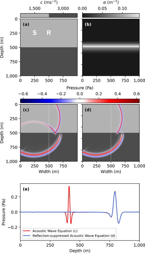
www.nature.com/scientificreports/
Figure 1. (a) The wave-speed of a 2 layer velocity-profile with point source location S and (b) local suppression
constant α( r ). (c) shows a snapshot of the wave-field at t = 0.35 s for the acoustic wave Eqs. (1, 2) and (d) the
reflection-suppressed wave Eqs. (3, 4), using a peak frequency of 50 Hz, 10 grid-points per smallest wavelength,
and a CFL20 number of 0.5. The resulting space interval and step-size become x = 1.0 m and t = 1.6 · 10−4
s, respectively. (e) shows a cross-section through snapshots (c) and (d) along the white dotted-line. A video of all
snapshots is available as supplementary material.
Results
First, we examine a medium with a sharp velocity contrast at geophysical scale (Fig. 1a). A point-source
Ricker19 wavelet with a peak frequency of 50 Hz is injected inside the medium, after which the wave-fields
arising from Eqs. (1) and (2) are compared with their reflection-suppressed counterparts (3, 4), with a value of
τmin = 4.68 · 10−3 s such that αmax = 0.14 m−1 (Fig. 1b).
In Fig. 1c,d,e we observe the effectiveness of the reflection suppression method via a snapshot and time series
display. Reflections at both small and large incident angles are fully suppressed, while the refracted wave-field
propagates with little to no perturbations.
The value of the suppression constant used in Fig. 1 was determined by a sensitivity assessment for the value
of τmin.
Figure 2 shows the level of suppression for different levels of τmin . Complete suppression of the reflections
seen in Fig. 1a is reached at a value of τmin = 4f10 , or αmax = 4cf1 0 . The level of suppression can be tuned depending
on the level of velocity contrasts in the medium or in the case when there exist specific regions where reflections
must be suppressed.
Next, we apply the same methodology in the ultrasound regime to a human skull m odel21 (Fig. 3a) with a
peak frequency of 200 kHz. We use a value of τmin = 7.80 · 10−7 s such that αmax = 855 m−1 (Fig. 3b).
In Fig. 3c,d,e we once again observe that the reflected wave-fields are very strongly suppressed, while the
transmitted wave-fields only exhibit small perturbations with respect to the unmodified acoustic wave equation.
Scientific Reports | (2022) 12:407 | https://doi.org/10.1038/s41598-021-04064-3 3
Vol.:(0123456789)
www.nature.com/scientificreports/
Figure 2. (a) The seismic trace, p( rS , rR , t), obtained from the simulation of Fig. 1 from a point probe at
location R (Fig. 1a) for different values of τmin. The first-arrival wave remains unaltered for all values of τ ,
whereas the subsequent reflected wave from the interface depends strongly on τ . Figure (b) highlights these
suppressed reflected waves compared to the unmodified acoustic wave equation (τmin = ∞). The suppressed
reflections yield an amplitude loss of − 14 dB for τmin = f10 , − 35 dB for τmin = 2f10 , and − 54 dB for τmin = 4f10 .
Lastly, we repeat the same procedure for the geophysical Marmousi22 model (Fig. 4a) at a peak frequency of
10 Hz. We use a value of τmin = 7.80 · 10−3 s such that αmax = 7.50 · 10−2 m−1 (Fig. 4b).
We once again observe a complete suppression of reflected wave-fields. The transmitted wave-field of the
modified acoustic wave equation in Fig. 4e contains varying perturbations with respect to the acoustic wave
equation. In part, these perturbations can be explained due to the wave-front in Fig. 4c containing both reflected
and transmitted wave-fields at heterogeneous locations, where Fig. 4d only contains the transmitted wave-field,
making it difficult to compare the two figures.
Discussion
The examples show that the method presented in this paper strongly suppresses internal reflections in a robust
manner, even within highly heterogeneous media. In addition, the transmitted wave-fields exhibit only small
perturbations. In order to fully remove these small perturbations, we recommend a combination of slowness
smoothing and a contrast-dependent α to keep changes to the transmitted wave-field to a minimum. If desired,
this method can also be used in conjunction with an impedance-matched wave equation, where the impedance
is kept constant throughout the medium, e.g: ρ(�r ) = c −1 (�r ). However, this will not allow for an independently
chosen density contrast and significantly affects the transmission amplitudes. A comparison between our method
and impedance matching is included in the supplementary information.
In general, the acoustic Poynting vector has shown to give an accurate estimate of the local propagation direc-
tion of wave-fields. However, problems may arise in the case of interfering waves. Firstly, we note that the use of
the acoustic Poynting vector as a measure of wave-field direction breaks down for interfering waves. Secondly,
and more importantly, we note that the modified Eq. (5) does not allow for reflection suppression in multiple
directions simultaneously. For this reason, more sophisticated wave-field decomposition methods would not
provide a solution to this issue. To remedy this, our method of contrast-dependent α allows interfering waves far
away from areas exhibiting large contrasts in wave-speed to propagate unaltered. Furthermore, at high-contrast
regions where interfering waves are known to appear, suppression could be turned off by setting α to zero locally.
As evident from the plane wave solution of Eqs. (3) and (4), it is possible for forward propagating components
of the wave-field not exactly aligned with Ŝ to also be suppressed. The losses incurred from such misalignments,
however, can be disregarded in general because of the exponential term in Eq. (6). Moreover, the results do not
show any occurrence of suppression of the forward propagating wave-field.
As an alternative to the acoustic Poynting vector, a-priori ray-based methods such as Eikonal solvers can be
used as a measure of the wave-field direction in the case of point-sources, by using the gradient of the shortest
travel time as a time-independent propagation direction vector. It is important to note that in this way only
primary arrivals are taken into account. Using this approach, the method presented here can also be applied in
the frequency domain. After temporally Fourier transforming Eq. (5) we obtain a modified Helmholtz equation,
which can subsequently be solved independently for each frequency component. Our experimental results using
Scientific Reports | (2022) 12:407 | https://doi.org/10.1038/s41598-021-04064-3 4
Vol:.(1234567890)www.nature.com/scientificreports/
Figure 3. (a) The wave-speed of a human skull model with point source location S and (b) local suppression
constant α( r ). (c) shows a snapshot of the wave-field at t = 7.44 · 10−5 s for the acoustic wave equation (1,
2) and (d) the reflection-suppressed wave equation (3, 4), using a peak frequency of 200 kHz, 10 grid-points
per smallest wavelength, and a C FL20 number of 0.5. The resulting space interval and step-size become
x = 2.45 · 10−4 m and t = 5.32 · 10−8 s, respectively. (e) shows a cross-section through snapshots (c) and
(d) along the white dotted-line. A video of all snapshots is available as supplementary material.
this approach show similar reflection suppression compared to the time domain method. Lastly, because PML’s
in the space-frequency domain only require a small modification to the spatial gradient term, the suppressing
term of Eq. (5) could conceivably also be implemented via PML’s inside the domain.
Computational costs for state-of-the-art FD wave simulations are of primary importance. The spatial interpo-
lation step used in this method keeps the added computational cost to a minimum, by only using values which
are already required to compute the derivatives of vx and vy . Further improvements in computational speed can
Scientific Reports | (2022) 12:407 | https://doi.org/10.1038/s41598-021-04064-3 5
Vol.:(0123456789)www.nature.com/scientificreports/
Figure 4. (a) The wave-speed of the Marmousi model with point source location S and (b) local suppression
constant α( r ). (c) shows a snapshot of the wave-field at t = 1.12 s for the acoustic wave equation (1, 2) and
(d) the reflection-suppressed wave Eqs. (3, 4), using a peak frequency of 10 Hz, 10 grid-points per smallest
wavelength, and a CFL20 number of 0.5. The resulting space interval and step-size become x = 5.70 · 10−4 m
and t = 5.18 · 10−4 s, respectively. (e) shows a cross-section through snapshots (c) and (d) along the white
dotted-line. A video of all snapshots is available as supplementary material.
be achieved by using adaptive scheme a pproaches23. Alternatively, Eq. (5) can be directly implemented using a
flux-limiter24 in a dimensional splitting approach. Results from both these methods are identical, but flux-limited
schemes are significantly more expensive computationally, and thus are not preferred. The implementation of
this method can also be extended naturally to the three dimensional case. Lastly, it is worth emphasising that
this approach consists of an analytical modification to the acoustic wave equation. Therefore, approaches to
Scientific Reports | (2022) 12:407 | https://doi.org/10.1038/s41598-021-04064-3 6
Vol:.(1234567890)www.nature.com/scientificreports/
numerical solutions are not limited to finite difference methods and could also be implemented using finite-
element or finite-volume methods.
Conclusion
The modification to the acoustic wave equation proposed in this paper successfully suppresses reflections within
heterogeneous media, while the transmitted wave-field only exhibits small perturbations. Using a staggered grid
FD scheme, the modified acoustic wave equation is implemented without significant additional computational
cost. In combination with the acoustic Poynting vector, the wave-field is essentially dynamically guided through a
reflection-less, heterogeneous medium. Although the solution is non-physical, this method is very suitable for use
in RTM, where internal reflections often lead to imaging artifacts. Additionally, this method could serve as a tool
for analysis purposes for many imaging methods, and could be used for any type of wave simulation application.
Received: 8 July 2021; Accepted: 10 December 2021
References
1. Baysal, E., Kosloff, D. D. & Sherwood, J. W. Reverse time migration. Geophysics 48, 1514–1524. https://doi.org/10.1190/1.14414
34 (1983).
2. Buur, J. & Kühnel, T. Salt interpretation enabled by reverse-time migration. Geophysicshttps://doi.org/10.1190/1.2968690 (2008).
3. Claerbout, J. F. Imaging the Earth’s Interior (Blackwell Scientific Publications Ltd, GBR, 1985).
4. Zhang, Y., Zhang, G. & Bleistein, N. Theory of true-amplitude one-way wave equations and true-amplitude common-shot migra-
tion. Geophysicshttps://doi.org/10.1190/1.1988182 (2005).
5. Fletcher, R. P., Fowler, P. J., Kitchenside, P. & Albertin, U. Suppressing unwanted internal reflections in prestack reverse-time
migration. In Geophysics, vol. 71. https://doi.org/10.1190/1.2356319. (Society of Exploration Geophysicists, 2006).
6. Yoon, K. & Marfurt, K. J. Reverse-time migration using the Poynting vector. Explor. Geophys. 37, 102–107. https://d oi.o rg/1 0.1 071/
EG06102 (2006).
7. Yoon, K., Guo, M., Cai, J. & Wang, B. 3D RTM angle gathers from source wave propagation direction and dip of reflector. SEG
Tech. Progr. Expand. Abstr. 30, 3136–3140. https://doi.org/10.1190/1.3627847 (2011).
8. Beniwal, S. & Ganguli, A. Defect detection around rebars in concrete using focused ultrasound and reverse time migration.
Ultrasonics 62, 112–125. https://doi.org/10.1016/j.ultras.2015.05.008 (2015).
9. Grohmann, M., Müller, S., Niederleithinger, E. & Sieber, S. Reverse time migration: Introducing a new imaging technique for
ultrasonic measurements in civil engineering. Near Surf. Geophys. 15, 242–258. https://d oi.o
rg/1 0.3 997/1 873-0 604.2 01700 6 (2017).
10. Johnson, J. L., Shragge, J. & van Wijk, K. Image reconstruction of multi-channel photoacoustic and laser-ultrasound data using
reverse time migration. In Photons Plus Ultrasound Imaging Sensing 2015, vol. 9323, 932314. https://doi.org/10.1117/12.2077220.
(SPIE, 2015).
11. Roy, O., Zuberi, M. A. H., Pratt, R. G. & Duric, N. Ultrasound breast imaging using frequency domain reverse time migration. In
Medical Imaging 2016: Ultrasonic Imaging and Tomography, vol. 9790, 97900B. https://doi.org/10.1117/12.2218366 (SPIE, 2016).
12. Filatova, V. M. & Nosikova, V. V. Determining sound speed in weak inclusions in the ultrasound tomography problem. Eurasian
J. Math. Comput. Appl. 6, 11–20. https://doi.org/10.32523/2306-6172-2018-6-1-11-20 (2018).
13. Virieux, J. & Operto, S. An overview of full-waveform inversion in exploration geophysics. Geophysics.https://doi.org/10.1190/1.
3238367 (2009).
14. Guasch, L., Calderón Agudo, O., Tang, M., Nachev, P. & Warner, M. Full-waveform inversion imaging of the human brain. npj
Digit. Med. 3, 1–12. https://doi.org/10.1038/s41746-020-0240-8 (2020).
15. Baysal, E., Kosloff, D. D. & Sherwood, J. W. Two-Way Nonreflecting Wave Equation. Geophysics 49, 132–141. https://doi.org/10.
1190/1.1441644 (1984).
16. Israeli, M. & Orszag, S. A. Approximation of radiation boundary conditions. J. Comput. Phys. 41, 115–135. https://doi.org/10.
1016/0021-9991(81)90082-6 (1981).
17. Virieux, J. P- SV wave propagation in heterogeneous media: velocity- stress finite-difference method. Geophysics 51, 889–901.
https://doi.org/10.1190/1.1442147 (1986).
18. Berenger, J. P. A perfectly matched layer for the absorption of electromagnetic waves. J. Comput. Phys. 114, 185–200. https://doi.
org/10.1006/jcph.1994.1159 (1994).
19. Ricker, N. The form and laws of propagation of seismic wavelets. Geophysics 18, 10–40. https://doi.org/10.1190/1.1437843 (1953).
20. Courant, R., Friedrichs, K. & Lewy, H. Über die partiellen Differenzengleichungen der mathematischen Physik. Math. Ann. 100,
32–74. https://doi.org/10.1007/BF01448839 (1928).
21. Iacono, M. I. et al. MIDA: A multimodal imaging-based detailed anatomical model of the human head and neck. PLoS One 10,
e0124126. https://doi.org/10.1371/journal.pone.0124126 (2015).
22. Versteeg, R. The Marmousi experience: Velocity model determination on a synthetic complex data set. Lead. Edge 13, 927–936.
https://doi.org/10.1190/1.1437051 (1994).
23. Yao, G., Wu, D. & Debens, H. A. Adaptive finite difference for seismic wavefield modelling in acoustic media. Sci. Rep. 6, 1–10.
https://doi.org/10.1038/srep30302 (2016).
24. Van Leer, B. Towards the ultimate conservative difference scheme. IV. A new approach to numerical convection. J. Comput. Phys.
23, 276–299. https://doi.org/10.1016/0021-9991(77)90095-X (1977).
Author contributions
E.V. conceived the experiment, T.S. developed and implemented the theory, T.S., L.H. and E.V. analyzed the
results. All authors reviewed the manuscript.
Competing interests
The authors declare no competing interests.
Additional information
Supplementary Information The online version contains supplementary material available at https://doi.org/
10.1038/s41598-021-04064-3.
Scientific Reports | (2022) 12:407 | https://doi.org/10.1038/s41598-021-04064-3 7
Vol.:(0123456789)www.nature.com/scientificreports/
Correspondence and requests for materials should be addressed to L.H.
Reprints and permissions information is available at www.nature.com/reprints.
Publisher’s note Springer Nature remains neutral with regard to jurisdictional claims in published maps and
institutional affiliations.
Open Access This article is licensed under a Creative Commons Attribution 4.0 International
License, which permits use, sharing, adaptation, distribution and reproduction in any medium or
format, as long as you give appropriate credit to the original author(s) and the source, provide a link to the
Creative Commons licence, and indicate if changes were made. The images or other third party material in this
article are included in the article’s Creative Commons licence, unless indicated otherwise in a credit line to the
material. If material is not included in the article’s Creative Commons licence and your intended use is not
permitted by statutory regulation or exceeds the permitted use, you will need to obtain permission directly from
the copyright holder. To view a copy of this licence, visit http://creativecommons.org/licenses/by/4.0/.
© The Author(s) 2022
Scientific Reports | (2022) 12:407 | https://doi.org/10.1038/s41598-021-04064-3 8
Vol:.(1234567890)You can also read


