A mathematical model and mesh-free numerical method for contact-line motion in lubrication theory
←
→
Page content transcription
If your browser does not render page correctly, please read the page content below
A mathematical model and mesh-free numerical method for
                                                              contact-line motion in lubrication theory
                                                                                Khang Ee Pang, Lennon Ó Náraigh1
                                                                  1 School   of Mathematics and Statistics, University College Dublin
                                                                                         (Dated: July 23, 2021)
                                                            We introduce a mathematical model with a mesh-free numerical method to de-
                                                         scribe contact-line motion in lubrication theory. We show how the model resolves the
arXiv:2107.10732v1 [physics.flu-dyn] 22 Jul 2021

                                                         singularity at the contact line, and generates smooth profiles for an evolving, spread-
                                                         ing droplet. The model describes well the physics of droplet spreading – including
                                                         Tanner’s Law for the evolution of the contact line. The model can be configured to
                                                         describe complete wetting or partial wetting, and we explore both cases numerically.
                                                         In the case of partial wetting, the model also admits analytical solutions for the
                                                         droplet profile, which we present here.

                                                                                        I.   INTRODUCTION

                                                       When a droplet of fluid (surrounded by a gaseous atmosphere) is deposited on a sub-
                                                   strate, it spreads until it reaches an equilibrium configuration. At equilibrium, the angle
                                                   between the liquid-gas interface and the solid surface is measured (conventionally, through
                                                   the liquid), to yield the equilibrium contact angle θeq . If the angle is less than 90◦ , the
                                                   substrate is deemed hydrophilic, whereas if the angle exceeds 90◦ , the substrate is deemed
                                                   hydrophobic [1]. Droplet spreading then describes the dynamic phase before the attainment
                                                   of this equilibrium.
                                                       In droplet spreading, the point of contact between the substrate and the gas-liquid inter-
                                                   face is in motion. And yet this contradicts the classical no-slip assumption in viscous fluid
                                                   flow, which stipulates that there should be no relative motion between a substrate in contact
                                                   with a fluid [2, 3]. The resolution of this paradox is that there is missing physics, and that
                                                   on a sufficiently small scale, there is slip, the dynamics of which are governed by the inter-
                                                   actions between the fluid molecules and the substrate molecules [4]. These molecular-level
                                                   interactions can be incorporated into a macroscopic fluid model via a so-called regulariza-
                                                   tion technique. Broadly, there are three regularization techniques in the literature – the slip
                                                   length [5], the precursor film [1], and the diffuse interface [6, 7]. Although methodologically
                                                   distinct, these yield the same qualitative and quantitative results when used to model droplet
                                                   dynamics. This consistency between the different approaches gives a solid justification for
                                                   the general approach of model regularization.
                                                       The purpose of this article is to introduce a novel model regularization, albeit one in the
                                                   spirit of those just described. The focus of the work is on mode regularization for the case
                                                   of thin-film flows (also called lubrication flows). For simplicity, we focus on two-dimensional
                                                   configurations (or equivalently, three-dimensional axi-symmetric configurations), however,
                                                   the generalization to three dimensions is straightforward.
                                                       Thin-film flows arise in the context of hydrophilic substrates, where the equilibrium shape
                                                   of the droplet is such that the typical size of the droplet base R greatly exceeds the maximum
                                                   droplet height h0 , leading to a small parameter  = h0 /R, with   1. In this context, the
                                                   Navier–Stokes equations reduce down to a single equation for the interface height (the so-
                                                   called Thin-Film Equation). In this context also, the interface height is conventionally
2

               FIG. 1. Schematic description of droplet spreading on a substrate

written as z = h(x, t). Thus, the coordinate x and is in the plane of the substrate, and the
z-coordinate is orthogonal to the substrate (e.g. Figure 1).

                                  Motivation for this work

   In the context of droplet spreading, the Thin-Film Equation inherits the contact-line
singularity from the full Navier–Stokes equations; the singularity can be regularized by
introducing a slip length [5, 8], or a precursor film [1, 9]. Both these regularizations
give accurate and consistent descriptions of contact-line spreading [10], albeit with some
drawbacks – the classical Navier slip-length model has a logarithmic stress singularity at
the contact line, while as the precursor-film model requires a precursor film to be present
that extends indefinitely beyond the droplet core. Although physically, such a precursor film
does exist, it has a very small thickness (10 − 100 nm [9]), meaning that such a small scale
must be resolved in the model: in particular, the numerical grid size must be at least as
small as the precursor-film thickness [11]. Furthermore, the resulting equations are quite stiff
numerically [12]. Although this approach is just about feasible for millimetre-scale droplets,
it may not be feasible for larger ones. Beyond the millimetre scale, an unphysically large
precursor-film thickness can be used in numerical investigations (and the results checked for
robustness to changes in the value of the precursor-film thickness), however, this approach
is somewhat unsatisfactory. The Diffuse Interface Model has been proposed as a more
general regularization of the contact-line singularity problem, valid for the full Navier–
Stokes equations beyond the lubrication limit [13]. The Diffuse Interface Model has been
implemented for droplet spreading in the thin-film lubrication approximation [6].
   Our contribution in this article is to introduce a novel regularization technique similar in
spirit to the Diffuse Interface Method – we formulate a theory of droplet spreading involving
a smooth interface height h, as well as a sharp interface height h, which interact via a
convolution operator and an evolution equation. In a previous work [14], the idea behind
this regularization was introduced in the context of thin-film lubrication flows – the so-
called Geometric Thin Film Equation. In the present article, we extend this previous work
by introducing a particle method as a novel and highly accurate solution method for the
Geometric Thin Film Equation. Also, Reference [14] was for complete wetting – in this work
we extend the Geometric Thin-Film Equation to describe partial wetting as well.
   The Geometric Thin-Film Equation can be viewed as special case of a mechanical
3

model for energy-dissipation on general configuration spaces – the derivation of the general
model involves methods from Geometric Mechanics such as Lie Derivatives and Momentum
Maps [15] – hence the name Geometric Thin-Film Equation. The main advantage of this
new method so far has been the non-stiff nature of the differential equations in the model,
which leads to robust numerical simulation results. A second advantage (the main focus of
the present work) is that the Geometric Thin-Film equation admits so-called particle solu-
tions. These give rise to an efficient and accurate numerical method (the particle method)
for solving the model equations.
    The basis for the particle method lies in the structure of the Geometric Thin-Film Equa-
tion: the model includes a ‘smoothened’ free-surface height h(x, t) and a ‘sharp’ free-surface
height h(x, t), related by convolution, h(x, t) = Φ ∗ h(x, t), where Φ ≥ 0 is a filter function
with a characteristic lengthscale
                               PN α. The model admits a delta-function solution for the sharp
free-surface height h(x, t) = i=1 wi δ(x − xi ), where δ is the Dirac delta function, and xi (t)
is the (time-dependent) centre of the Delta function. The delta-function centres {xi (t)}N  i=1
satisfy a set of ordinary differential equations:
                          dxi
                              = Vi (x1 , · · · , xN ),   i ∈ {1, 2, · · · N },                 (1)
                          dt
where Vi is a velocity function which can be derived from the Geometric Thin-Film
                                                                              PN        Equation.
Thus, the screened free-surface height admits a regular solution h(x, t) = i=1 wi Φ(x − xi ).
In this context, the weights wi and the delta-function centres xi (with i ∈ {1, 2, · · · , N }) can
be viewed as pseudo-particles, which satisfy the first-order dynamics (1). We will demon-
strate in this article another advantage of this particle-method: it is a mesh-free method that
automatically accumulates particles in regions where |∂xx h| is large, thereby mimicking the
effects of adaptive mesh refinement, with none of the computational overheads associated
with that method.
               PN A final key advantage of the particle method is positivity-preservation:
as h(x, t) =      i=1 wi Φ(x − xi ), with wi ≥ 0 and Φ ≥ 0, the numerical values of h(x, t)
are guaranteed never to be negative, hence the numerical method is manifestly positivity-
preserving.

              This work in the context of Environmental Fluid Mechanics

   Before introducing the method, we place the method in the context of Environmental
Fluid Mechanics, focusing in particular on droplet spreading on plant leaves. In general,
surfaces can be further classified as being (i) super-hydrophobic (θeq > 150◦ ), hydrophobic
(90◦ < θeq < 150◦ ), hydrophilic (10◦ < θeq < 90◦ ), or super-hydrophilic (θeq < 10◦ ). Plant
leaves display this wide range of contact angles. Superhydrophobic surfaces have been
frequently found in wetland plants, where the superhydrophobic surface prevents a buildup
of water on the leaves, which could otherwise promote the growth of harmful micro-organisms
and limit the gas exchange necessary for photosynthesis [16].
   A particularly well-studied plant with superhydrophobic a leaf surface is the Lotus plant
(Nelumbo nucifera), with a contact angle of about 160◦ [16, 17]. The leaves of the Lotus
plant also demonstrate a low contact-angle hysteresis, such that water droplets roll off the
leaf surface when at a low tilt angle (4◦ ). During rolling, contaminating particles are picked
up by the water droplets, and are then removed with the droplets as they roll off [16].
The leaf structure of the Lotus plant has been studied using Scanning Electron Microscopy,
and reveals a hierarchical microstructure made up of micron-scale pillars (cell papillae) and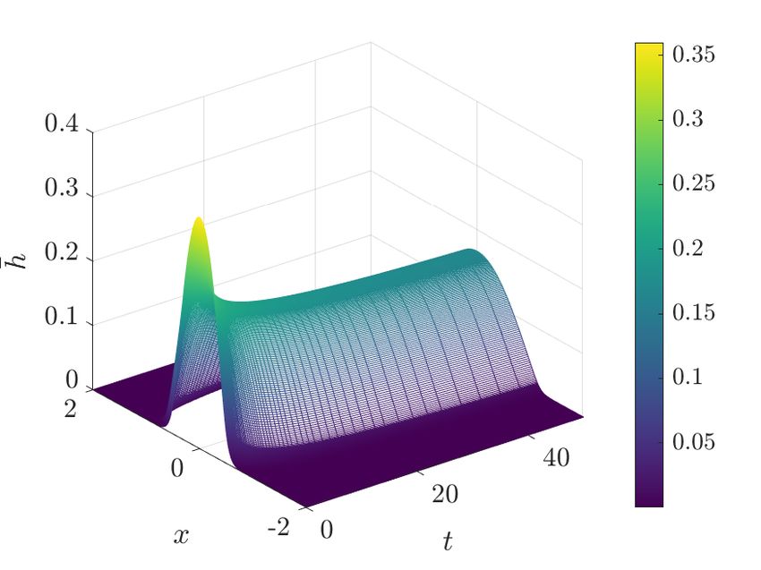
4

    FIG. 2. A species of carnivorous plants of the genus Nepenthes (image: Khang Ee Pang)

a randomly covered by a smaller branch-like nanostructure [18] (the wax crystal, with mi-
crostructures ∼ 100 nm in diameter) [19]. Such biological microsturctures are the inspiration
for engineered super-hydrophobic surfaces [19].
   In contrast, plants with superhydrophilic leaf surfaces are often found in tropical re-
gions [20]. A water droplet that spreads on a superhydrophilic surface will spread and form
a wide, flat droplet – effectively a thin film. Evaporation in such films is more efficient than
in a spherical droplet, due to the increase of the water-air interface. Thus, water evaporates
from a superhydrophilic leaf much faster than that from a hydrophilic or superhydrophobic
one, thereby keeping the leaf dry, reducing the accumulation of harmful micro-organisms
on the leaf surface, and increasing the gas exchange with the environment, for the purpose
of photosynthesis [16]. A well-studied hydrophilic plant is Ruellia devosiana, wherein the
superhydrophilic property of the leaf surface is due both to the leaf microstructure, and to
a secretion of surfactants by the leaf, which both promote spreading [21].
   Other plants which exploit hydrophilicity are the carnivorous plants of the Nepenthes
genus (e.g. Figure 2), the perisotone of which is a fully wettable, water-lubricated anisotropic
surface [22]. Insects landing on the peristone or rim of the plant effectively ‘aquaplane’ down
the plant rim [22] before being captured by the viscoelstic fluid inside the pitcher [23].
   We emphasize here that both the super-hydrophobic and super-hydrophilic plant surfaces
are extreme cases. In a comprehensive investigation of 396 plant species out of 85 families
growing in three different continents at various elevations (including 792 leaf surfaces total),
only forty leaf surfaces (5.1% out of 792) were found in these extremes, including 24 super-
hydrophobic surfaces and 16 super-hydrophilic surfaces [20]. Thus, most leaf surfaces lie
inside these extremes. The droplet-model introduced in this paper is most relevant to
hydrophilic cases where the equilibrium contact angle is small.

                                      Plan of the paper

   In Section II we present the classical Thin-Film Equation as a model of droplet spreading.
Certainly, this is a very well-established topic, however, we include a summary of this topic
here because it enables us to clearly mark out the point of departure of the present work.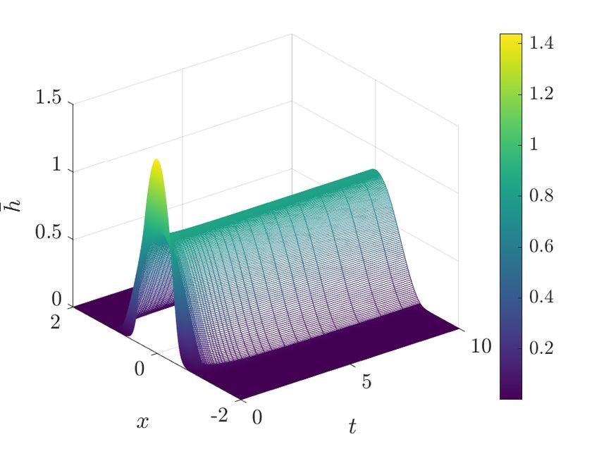
5

Thereafter, in Section III we introduce the Geometric Thin-Film Equation as a regularized
model which enables contact-line motion. In Section IV we introduce the particle method
for generating numerical solutions of the Geometric Thin-Film Equation. In Section V
we presents results for complete wetting. In Section VI we demonstrate how the Geometric
Thin-Film Equation can be extended to the case of partial wetting, and we present numerical
results for that case also. Concluding remarks are given in Section VII.

                        II.    REVIEW OF CLASSICAL THEORY

   In this section we review the classical theory of the Thin Film Equation, including the
problem of the contact-line singularity. The purpose of this review is to put the Geometric
Thin-Film Equation into the context of the classical theory; the theoretical formulation of
the Geometric Thin-Film Equation is therefore presented subsequently in Section III.

                                 Classical Thin-Film Equation

   We review the derivation of the classical Thin Film Equation for a flow in two dimensions,
with spatial coordinates x and z (we refer the reader Reference [24] for the details). The
starting-point is the kinematic condition valid on the free surface z = h(x, t):
                              ∂h                  ∂h
                                 + u(x, z = h, t)    = w(x, z = h, t).                       (2)
                              ∂t                  ∂x
The fluid flow is assumed to be incompressible, such that ux + vy = 0. The incompressiblity
condition can be integrated once to give
                                        Z h
                                            ∂u
                     w(x, z = h, t) = −        dz,    z(x, z = 0, t) = 0.               (3)
                                         0 ∂x

Equations (2)–(3) can be combined to give
                                                           Z   h
                              ∂h ∂q
                                 +    = 0,            q=           u(x, z, t) dz.            (4)
                              ∂t   ∂x                      0

In the lubrication limit, the velocity u(x, z, t) satisfies the equations of Stokes flow, hence

                                     ∂P    ∂ 2u                    ∂P
                                 −      + µ 2 = 0,                    = 0,                   (5)
                                     ∂x    ∂z                      ∂z
where P is the fluid pressure and µ is the constant dynamic viscosity. We integrate the first
equation of the pair in (5) once with respect to z to obtain
                                            h
                                       ∂u           1 ∂P
                                                =        (h − z) .                           (6)
                                       ∂z   z       µ ∂x

The standard interfacial condition is that the viscous stress ∂u/∂z should vanish on the free
surface z = h(x, t). Thus, Equation (6) becomes ∂u/∂z = µ−1 (∂p/∂x)(z − h). Applying the
no-slip boundary condition
                                      u(x, z = 0, t) = 0,                                 (7)
6
the u-velocity profile becomes
1 ∂P 1 2
u(x, t) = 2
z − hz , (8)
µ ∂x
hence
1 3 ∂P
q=− h . (9)
3µ ∂x
The pressure P is identified with the Laplace pressure, P = −γ∂xx h, where γ is the surface
tension and hxx is the interfacial curvature in the longwave limit. Hence, Eqution (9)
becomes:
γ 3
q= h hxxx . (10)
3µ
Substituting Equation (10) into Equation (4) gives:
3
∂h γ ∂ 3∂ h
+ h = 0. (11)
∂t 3µ ∂x ∂x3
Contact-Line Singularity
In the context of droplet spreading, it is desirable to propose a similarity solution to
Equation (11), corresponding to a self-similar droplet that retains some overall structural
properties even as the base of the droplet spreads out. Dimensional analysis indicates that
the similarity solution should be:
x/R
h(x, t) = h0 (t/t0 )−1/7 f (η), η= , (12)
(t/t0 )1/7
where h0 and R are as given in Figure 1 and t0 is a timescale to be determined. Substitution
of Equation (12) into Equation (11) yields:
3
γ t0 h0
1
7
ηf = f 3 f 000 . (13)
3µ h0 R
The timescale t0 is chosen to be the capillary timescale, such that (γ/3µ)(t0 /h0 )(h0 /R)3 = 1.
Thus, Equation (13) becomes:
1
7
ηf = f 3 f 000 . (14)
The appropriate droplet-spreading boundary conditions for Equation (14) are f (0) = 1,
f 0 (0) = 0,
f = f 0 = 0, at η = η0 > 0, (15)
where η0 corresponds to the outermost extent of the droplet. Thus, the position a at which
the (microscopic) contact line touches down to zero is described by a(t)/R = η0 (t/t0 )1/7 .
Unfortunately, the similarity solution (12) with the boundary conditions (15) fails to exist;
instead, f (η) degenerates into a Dirac delta function centred at η = 0, and the droplet does
not spread [25].
The reason for this failure is that the no-slip condition (7) is inconsistent with the phe-
nomenon of droplet spreading. When the model (11) is applied to droplet spreading, the7
physics which permits slip to occur on sufficiently small scales is missing. The missing
physics is then put into the model as part of a regularization. For instance, by allowing for
slip on a sufficiently small scale `, Equation (11) becomes:
3
∂h γ ∂ 1 3 2 ∂ h
+ h + `h = 0. (16)
∂t µ ∂x 3 ∂x3
Equation (16) is the Thin-Film Equation with a slip-length model.
Using the theory of matched asymptotic expansions, it has been shown [26] that the
solution of Equation (16) consists of an outer solution and an inner solution. The outer
solution resembles the similarity solution (12) and is valid on large scales, far from the
contact line. The inner solution is valid on small scales close to the contact line, and
provides for contact-line motion. Indeed, by matching the inner and outer solutions across an
intermediate matching zone, the contact-line a(t) is shown to satisfy the so-called Tanner’s
Law,
γθ03 R6
da 2a
= 1 + 2 − ln a−6 . (17)
dt 3µ R
Where θ0 is the initial contact angle. Thus, a(t) ∼ t1/7 , which is the scaling that would be
expected if the similarity solution could be made to extend down to the microscopic scale.
The slip-length model therefore provides for a resolution of the contact-line singularity.
However, the stress γhxx remains singular at the contact line. For these reasons, an alterna-
tive regularization of the Thin-Film Equation has been proposed, namely the Precursor-Film
model [1, 9]. Following Reference [14], in this work we present the Geometric Thin-Film
Equation as an alternative regularization, the advantage of this approach as we reveal in
subsequent sections is the remarkable simplicity of the numerical solutions produced by this
model.
III. GEOMETRIC THIN-FILM EQUATION: THEORETICAL FORMULATION
In the framework of the Geometric Thin-Film Equation, the starting-point is the assump-
tion that there is missing physics on a small scale. Instead of modelling the missing physics,
it is parametrized. As such, h(x, t) is used to denote the interface location in a crude model
with missing physics – which we call here the ‘noisy’ interface location. The noisy interface
location is to be smoothened by a filtering operation, to produce a smoothened, more ac-
curate, estimate of the interface location, which we denote by h(x, t). The noisy interface
location may be different from the true interface location – for instance, the noisy interface
location may be zero, whereas the true interface location may be close to, but different
from zero – as would be the case if the noisy interface location was obtained through an
incomplete model with missing small-scale physics.
Model A
To take account of the fact that h represents a smoother description of the interface
location than h, we propose that h and h be connected via the expression
h = h + η, (18)8
where η is a fluctuating quantity with mean zero and variance σ 2 . Then, h(x, t) can be made
into an accurate estimate of the interface location by minimizing the total interfacial energy
Z ∞q
E[h] = γ 1 + |∂x h|2 dx, (19)
−∞
subject to a fixed-variance-constraint:
Z ∞
|h − h|2 dx = σ 2 . (20)
−∞
Here, γ is a positive constant representing the surface area; the constraint (20) enforces
a fixed level of uncertainty between the model with missing physics and the smoothened
model.In practice, we minimize the surface area in the long-wave limit: instead of Equa-
tion (19) we minimize Z ∞
E[h] = 12 γ |∂x h|2 dx, (21)
−∞
which is obtained from Equation (19) in the longwave limit, when |∂x h|2 is small.
Equation (21) with constraint (20) is a constrained minimization problem – to solve it,
one would introduce an energy functional with a Lagrange multiplier:
Z ∞
1 2 1 2
L[h, h] = E[h] + λ 2 |h − h| dx − 2 σ . (22)
−∞
One would then compute
δL δL
= 0, = 0, (23)
δh δh
yielding
− γ∂xx h − λ(h − h) = 0, h − h = 0. (24)
In practice, solving Equation (24) yields inconsistent results, as it implies that h = h. But
h and h live in different function spaces (h is noisy, h is smooth), so Equation (24) cannot
be correct. Instead, we can study the dynamics, whereby L[h, h] in Equation (22) gradually
evolves to a minimum configuration over time. The dynamics are highly conditioned:
• The evolution of h and h must be such that L tends to a minimum over time;
R∞ R∞
• The integrals −∞ h(x, t)dx and −∞ h(x, t)dx must be conserved quantities, reflecting
underlying principles of conservation of fluid mass.
Under these conditions, the evolution equation for h must be of a generic conservative-
gradient-descent type, hence:
∂h ∂ ∂ δL
= hM . (25)
∂t ∂x ∂x δh
where M ≥ 0 is a mobility function to be determined. The evolution equation for h may
be similar. However, for simplicity, we may assume that h relaxes instantaneously to a
smoothened form of h, hence δL/δh = 0, hence
− γ∂xx h = λ(h − h), (26)9
or −1
γ
h = 1 − ∂xx h. (27)
λ
Equation (27) establishes a natural smoothing operation and hence, smoothing kernel for the
formulation, namely, the Helmholtz kernel. Substitution of Equation (26) into Equation (25)
yields:
∂h ∂ ∂
=− hM γ∂xx h . (28)
∂t ∂x ∂x
The physical model for h is completed by specifying the mobility. This is done by reference
to the classical theory in Section II. However, instead of M = (1/3µ)h2 we take
1 2
M= h; (29)
3µ
2
the reason for using h in the mobility becomes apparent when we look at particle-like
solutions of the regularized model (Section IV). Finally, the value of the Lagrange multiplier
λ is chosen at each point in time to reflect the model uncertainty:
−1 2
Z ∞
1
1 − ∂xx h − h dx = σ 2 . (30)
−∞ λ
We refer to this model with a fixed level of uncertainty as Model A.
Model B
In practice, recomputing the Lagrange multiplier λ at each time t is a difficult task nu-
merically. However, an equivalent model can be formulated by introducing an unconstrained
functional, Z ∞
1 γ
L[h, h] = E[h] + 2 2 (h − h)2 dx. (31)
α −∞
Here, the parameter α corresponds to model uncertainty on the (small) lengthscale λ. The
dynamical equation is the same as before (Equation (28)), as is the mobility; however, now
h is computed as
−1
h = 1 − α2 ∂xx h := K ∗ h. (32)
We refer to this model with uncertainty on a small scale α as Model B. Here, we have
introduced the standard notation for smoothing kernels:
Z ∞
2 −1
K ∗ f (x) = (1 − α ∂xx ) f (x) = K(x − y)f (y)dy,
−∞
and we explicitly use K for the Helmholtz kernel, such that
1 −α|x|
K(x) = e .
2α10
Although Model A and Model B are different, there is a one-to-one relationship between
them, and they are equivalent – e.g. λ in Equation (30) is clearly a [lengthscale]2 which
depends on time. We therefore identify
α(t) = [λ(t; σ)]−1/2 , (33)
and the required uncertainty on a small lengthscale α in the second description of the model
is the average value of Equation (33):
1 ∞
Z
α = lim [λ(t; σ)]−1/2 dt. (34)
T →∞ T 0
Due to the computational efficiency, Model B is preferred in this work.
The kernel solution (32) can be substituted back into the expression L[h, h] to give:
h Z ∞h
2
−1 i 1 2 2
2 i
`[h] := L h, h = 1 − α ∂xx h = 2γ ∂x h + α ∂xx h dx. (35)
−∞
This can in turn be written in several further ways:
1. The inner-product pairing of ∂x h with ∂x h:
Z ∞
1
`[h] = 2 γ ∂x h∂x h dx. (36)
−∞
2. The weighted inner-product pairing:
Z ∞
1 1
∂x h 1 − α2 ∂x2 ∂x h dx.
`[h] = 2
γh∂x h, ∂x hiK = 2
γ (37)
−∞
The pairing h·, ·iK defines a Reproducing Kernel Hilbert Space [27].
Equation (28) now reads:
∂h ∂ ∂ δ`
=− hM , h = K ∗ h. (38)
∂t ∂x ∂x δh
Higher-order smoothing
For the purpose of generating particle-like solutions of the regularized model (e.g. Sec-
tion IV), smoothing with the Helmholtz kernel is not sufficient. Therefore, in this paper,
we work with a higher-order smoothing. We take ` as before (specifically, Equation (35)),
with evolution equation (38) and smoothing kernel h = K ∗ K ∗ h – this is a straightforward
extension of the basic model. We therefore summarize in one place the model studied in
this work:
Z ∞
1
`[h] = 2 γ ∂x h∂x h dx, (39a)
−∞
h = K ∗ K ∗ h, (39b)
∂h ∂ ∂
=− hM ∂xx h . (39c)
∂t ∂x ∂x
The aim of the remainder of the paper is to explore numerically the solutions of Equation (39)
– we will use Φ = K ∗ K to denote the double Helmholtz kernel, such that h = Φ ∗ h – the
need for this higher-order smoothing will become apparent in Section IV.11
Discussion
Summarizing our work so far, we have introduced a regularized thin-film equation where
the missing small-scale physics is not modelled, but is instead parametrized. The idea of
the model is that h(x, t) provides an incomplete description of the droplet evolution (but
which nonetheless contains important physical information, such as the problem dependence
on the viscosity µ and time t. A refined description of the interface is then obtained via a
smoothened interface profile h = Φ ∗ h. Overall, the model evolves so as to minimize the
interfacial energy (area) while keeping the difference between h and h as small as possible.
The model as formulated envisages that h(x, t) is an incomplete description of the inter-
face profile (with missing small-scale physics). The missing physics is encoded either as a
fixed level of uncertainty between h and h (model A), or such that the uncertainty in the
model description occurs below a lengthscale α (model B). These two models are equivalent,
although model B is preferred for computational simplicity.
The equation (39) is a variant of the so-called Geometric Thin-Film equation introduced
in Reference [14]: by viewing a = hdx as a one-form, Equation (39) can be written as
∂a
= −£U (a), (40)
∂t
where £U (a) = £U (hdx) = ∂x (U h) dx is the Lie derivative on one-forms; in this instance,
U = M ∂x (δ`/δh) is the pertinent vector field. Equation (40) is then a very simple instance
of a general theory of gradient-flow dynamics [15] which uses geometric mechanics (Lie
Derivatives, Momentum Maps) to formulate an energy-dissipation mechanical model for
general configuration spaces – hence the Geometric Thin-Film equation. Equation (39)–(40)
can furthermore be identified as a special case of Darcy’s Law [15], where the generalized
force is f = −∂x (δ`/δh), the Darcy velocity is U = M f , and the flux-conservative evolution
is equation for the conserved scalar quantity h is ht + ∂x (hU ) = 0. These insights will be
used in formulating the Geometric Thin-Film equation for the case of partial wetting in
Section VI, below.
We remark finally here on the intriguing connection between Model A and ‘denoising’
in Image Processing – in Image Processing one is given a noisy image h and it is desired
to produce a smoother image h while keeping the difference between the noisy and the
smooth image at a fixed level σ. This is achieved by minimizing a functional such as
Equation (22) [28, 29]. Our evolution equation (28) for the free-surface height h(x, t) in a
thin-film flow is equivalent to carrying out denoising on a (one-dimensional) image in Image
Processing.
IV. GEOMETRIC THIN-FILM EQUATION: PARTICLE SOLUTIONS
The general theory of geometric dissipative mechanics introduced in Reference [15] in-
cludes many examples where discrete, particle-like solutions (such as Equation (1)) are
admitted. Motivated by these examples, we seek simplified solutions of Equation (39) of the12
following form:
N
X
hN = wi δ(x − xi (t)), (41a)
i=1
N
N X
h (x, t) = wi Φ(x − xi (t)). (41b)
i=1
where N is a positive integer corresponding to a truncation of an infinite sum, wi ≥ 0 are
weights to be computed, and δ(·) is the Dirac delta function. The motivation for seeking
out such highly simplified particle solutions is that they make the task of solving the partial
differential equation (39) numerically very simple: instead of discretizing a fourth-order
parabolic-type partial differential equation and solving it numerically, we can instead solve
a set of ordinary differential equations for the delta-function centres xi (t) using standard
time-marching algorithms. This simplifies the numerical computations greatly. We refer to
the weights wi together with the delta-function centres xi (t) as the ‘particles’ – thus, we are
concerned with a particle-solution of Equation (39). We describe the construction of such
particle-solutions in what follows.
The weights wi ≥ 0 are chosen such that
Z ∞ Z ∞
N
lim h (x, t = 0)φ(x)dx = h0 (x)φ(x)dx, (42)
N →∞ −∞ −∞
where φ(x) is an arbitrary smooth, integrable test function. This limit can be satisfied by
taking
0 N 2L
xi (t = 0) = xi = i − , i ∈ {1, 2, · · · N }, (43)
2 N
where L is a lengthscale such that supp(h0 ) ⊂ [−L, L], and by taking
wi = h0 (x0i )(2L/N ), i ∈ {1, 2, · · · N }, (44)
then, Equation (42) is satisfied automatically.
We now multiply both sides of Equation (39) by the test function φ(x), integrate from
x = −∞ to x = ∞, and apply vanishing boundary conditions at these limits. We thereby
obtain γ 2
hφ, ht i − hφx , hh ∂xxx hi = 0, (45)
3µ
where h·, ·i denotes the standard pairing of square-integrable functions:
Z ∞
hf, gi = f gdx, f, g, ∈ L2 (R). (46)
−∞
We substitute Equations (41) into Equation (45). Owing to the judicious choice of mobil-
2
ity M = (1/3µ)h (cf. Equation (29)), no instance of the singular solution hN (x, t) gets
N
squared (only the smoothened solution h gets squared). After performing some standard
manipulations with Dirac delta functions, Equation (45) becomes:
N N
X dxi γ X h N N
i
wi φx (xi ) − wi φx (xi ) (h )2 ∂xxx h = 0, (47)
i=1
dt 3µ i=1 x=xi13
N N
where now [(h )2 ∂xxx h ]x=xi is taken to mean
"X
N
#2 " N
#
X
wj Φ(x − xj ) wj Φ000 (x − xj ) . (48)
j=1 j=1 x=xi
Equation (47) is re-arranged to give
N
X dxi γ h N 2 N
i
wi φx (xi ) − (h ) ∂xxx h = 0. (49)
i=1
dt 3µ x=xi
Equation (49) is true for all test functions φ(x) and all initial data h0 (x) (hence wi ), hence
dxi γ 2
− h ∂xxx h = 0. (50)
dt 3µ x=xi
Thus, Equation (41), together with the ordinary differential equations
dxi γ 2
= h ∂xxx h , t > 0, i = 1, 2, · · · , N, (51)
dt 3µ x=xi
and initial data
N
xi (t = 0) = x0i = i− (2L/N ), supp(h0 ) ⊂ [−L, L], (52)
2
give a so-called singular solution to the Geometric Thin-Film Equation (39). The centres of
the Dirac delta functions xi (t) with associated weights wi are identified as pseudo-particles,
and the velocity Vi of the ith pseudo-particle is identified with the right-hand side in Equa-
tion (51),
dxi γ 2
= Vi (x1 , · · · , xN ), Vi (x1 , · · · , xN ) = h ∂xxx h . (53)
dt 3µ x=xi
Key properties of the particle evolution equations
We notice that in Equation (53), evaluation of Φ000 is required – this is the rationale
for our choice of the double Helmholtz kernel as the smoothing kernel in Equation (39).
Using the single Helmholtz kernel K would not be sufficient,P as K 000 is singular at the origin.
Furthermore, as the reconstructed interface profile h(x, t) = N i=1 wi Φ(x−xi (t)) involves the
positive weights wi and a positive kernel Φ ≥ 0, the particle method is positivity-preserving:
if h and h are initially positive, then the stay positive for all time. The numerical particle
method is manifestly positivity-preserving, this is a key advantage as a numerical method
that led to erroneous negative values of h and h would produce unphysical results.
Numerical Solutions using the Particle Method
In this paper, we solve the Geometric Thin-Film Equation (39) numerically using the
particle method (53). To demonstrate the accuracy of the novel particle method, we compare14
the particle method to a standard fully-implicit finite-difference method. It can be noted
from the particle method (specifically Equation (53)) that N ordinary differential equations
are to be solved; each of the N right-hand-side (RHS) terms requires a summation over all
other particles (cf. Equation (41b) and the second entry in Equation (53)) – this suggests
the particle method has computational complexity O(N 2 ). However, the number of floating-
point operations to be performed in evaluating the different RHS terms can be dramatically
reduced by symmetry operations, to give an overall computational complexity O(N ) – this
is the so-called fast-particle method. We give details of the fast particle method and our
fully-implicit finite-difference method in Appendix A.
Both the particle method and the fully-implicit finite-difference method are solved in
Matlab. The particle method makes use of Matlab’s built-in time-evolution algorithms for
ordinary differential equations, notably, ODE45 and ODE15s.
V. COMPLETE WETTING
In this section we present numerical results for complete wetting for the Geometric Thin-
Film Equation. Equation (39) R ∞clearly corresponds to the case of complete wetting: the
energy functional E = (1/2)γ −∞ |∂x h|2 dx is penalized, meaning that the system evolves to
minimize the curved part of the droplet interface, that is, the part of the droplet interface
in contact with the surrounding atmosphere.
Non-dimensionalization and Initial Conditions
To characterize this spreading phenomenon, we solve the Geometric Thin-Film equa-
tion (39) in dimensionless variables. The interfacial height is made dimensionless on a length-
scale h0 , which is proportional to the initial maximum droplet height hmax . In this section,
we take the rather non-standard value h0 = (8/3)hmax for h0 , this is done here to compare
with Reference [14]. The x-coordinate is then made dimensionless on the initial droplet
base L. Finally, time is made dimensionless on the capillary timescale τ = (3µL/γ)(L/h0 )3 .
The ratio = h0 /L must be small, for inertial effects to be negligible, and hence, for the
lubrication theory underlying Equation (39) to be valid. Henceforth, we assume that all of
the relevant variables have been made dimensionless in this way. The initial condition for
the droplet height therefore reads:
( h 2 i
3 1
− x 2
, if |x| < 12 ,
h(x, t = 0) = 2 2 (54)
0, otherwise.
Thus, the droplet area (which is the analogue of droplet volume in two dimensions) is
therefore fixed as Z
h(x, t = 0) dx = 1/4.
R R
Both the droplet area h(x, t) dx and h(x, t) dx are conserved under the evolution equa-
tion (39). The simulations are carried out in a finite spatial domain x ∈ [−2, 2] with periodic
boundary conditions – this condition also establishes the limits of integration on the forego-
ing integrals.15
Results
We solve Equation (39) with the initial condition (54). The numerical calculations in-
dicate that the particle method and the finite-difference method produce results that are
qualitatively the same: we therefore show only results for the particle method. A rigorous,
quantitative comparison between the two methods is also presented herein – this analysis
also justifies the number of particles used in the calculations as N = 800, this can be deemed
equivalent to a grid spacing of ∆x = 2L/N = 0.005 in the finite-difference method.
A first set of results is shown in Figure 3. In Figure 3(a) we show a space-time plot of the
smoothened free-surface height h̄ where the spatial grid is evaluated at the particle positions
xi (t) – effectively, a discretization of h on a non-uniform grid. From this plot, region in space
where where h is significantly different from zero increases over time, demonstrating that
the droplet is indeed spreading. Figure 3(b) shows a snapshot the filtered surface height
and its slope at t = 50. The particle locations are shown explicitly in Figure 3(b) – there is
FIG. 3. (a) Space-time plot of h̄(x, t) showing the spreading of the droplet. (b) Droplet shape h̄
and the slope ∂x h̄ at t = 50.
a high concentration of particles in the regions of high curvature – this is discussed in more
detail in what follows.
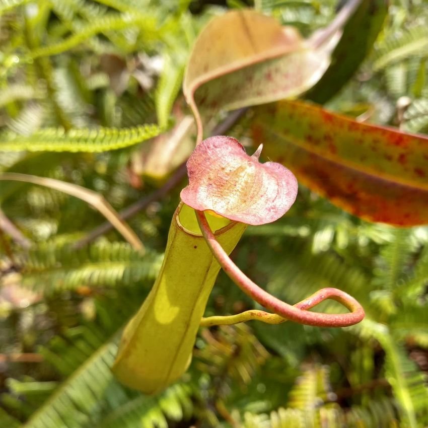
In Figure 4, we plot the particle trajectories xi (t) for the solution of the Geometric Thin-
Film Equation via the particle method. Intriguingly, the particles are seen to accumulate at
regions where |∂xx h| is large, giving a higher spatial resolution in regions of high interfacial
curvature. When a finite-difference or finite-volume solver is able to execute local grid
refinement in regions of where the spatial derivatives are large in magnitude, this is because
of adaptive mesh-refinement, which is a complex and computationally expensive feature to
add to a numerical solver. Here, the particle method demonstrates a built-in tendency to
mimic the effect of adaptive mesh-refinement, without the high computational overhead of
that method. Furthermore, in Figure 4 we have used the built-in MATLAB ODE solvers
to generate the space-time plot, meaning that the adaptive mesh refinement is performed in
the temporal as well as the spatial domain.
A further advantage of the particle method is that it provides a numerical description
of the contact line by simply following the trajectory of a particle starting near the contact
line, say xk (t) such that xk (0) = 0.5. This is also shown in Figure 4, where the contact line
is found to satisfy Tanner’s Law, with xk (t) ∼ t1/7 .16
FIG. 4. Evolution of the particle trajectories xi (t) (logarithmic scales on both axes). The colors
indicate the weight corresponding to each particle wi . The line t1/7 is imposed to show that the
trajectories follows a power law at late time.
The finding that the Geometric Thin-Film Equation satisfies Tanner’s Law of droplet
spreading indicates that the regularized model is capturing the large-scale physics in the
droplet-spreading problem. In order to demonstrate this even further, we introduce the
function fα (η, t) = t−1/7 h(ηt1/7 , t), with ηt1/7 = x. In Figure 5 we produce a space-time plot
of fα (η, t) – this is seen to relax to a constant profile at late times as t → ∞. Furthermore,
FIG. 5. Space-time plot in similarity variables of fα (η, t) = t−1/7 h(ηt1/7 , t).
the profile of fα (η, t) at fixed t (t large) can be compared with a similarity solution of the
unregularized problem, f 3 f 000 = ηf /7 (cf. Equation (14)). This ordinary differential equation
is then solved with the shooting method together with appropriate initial conditions [14].17
The results are shown in Figure 6. This figure therefore shows that the Geometric Thin-Film
FIG. 6. Comparison between fα (η, t = 50) and the similarity solution, solved using the shooting
method.
Equation describes the expected large-scale droplet-spreading physics in the droplet core.
Where the classical Thin-Film Equation breaks down at the contact line, the height profile
of the Geometric version decays smoothly to zero.
Rigorous Error and Performance Analysis
We analyse the truncation error associated with the standard fully-implicit finite-
difference method and the particle method. As such, let h denote the exact solution of
Equation (39), and let h∆x denote the numerical solution with step size ∆x (finite-difference
method), or number of particles N = 2L/∆x (particle method). We assume that the error
kh − h∆x k depends smoothly on ∆x, then
kh − h∆x k = C∆xp + O(∆xp+1 ), (55)
for some constant C and p. Since h is unknown, we instead compute
ε(∆x) := kh∆x − h∆x/2 k (56)
Using the triangle inequality, it can be shown that
ε(∆x) ≤ C∆xp (1 − 1/2p ) + O(∆xp+1 ). (57)
We take the natural logarithm on both sides of Equation (57); this gives:
log ε ≤ p log(∆x) + log(C) + log(1 − 1/2p ). (58)
Thus, the rate of convergence (or the order of accuracy) of the numerical method is p; p can
be computed from the numerical simulations as the slope of the log-log plot between the
error ε and the grid spacing ∆x.18
Figure 7 shows the rate of convergence of the finite-difference method and the particle
method – here we use the L1 norm applied to Equation (57)–(58) (our choice of norm is
obtained because the particle solutions are expected to converge weakly in an L1 function
space, see Reference [30]). The finite-difference method is implemented with a step size of
∆t = 0.01, while the particle method uses the ODE45 solver in Matlab, hence an adaptive
time step. Both methods use the same numerical parameter of, α = 0.05, with final time
T = 1, and periodic boundary condition on the spatial domain x ∈ [−1, 1]. From this
figure, both the particle method and the standard finite-difference method are estimated to
be second-order accurate in the spatial domain.
FIG. 7. Convergence plot of the finite-difference method (left) and the particle method (right).
Furthermore, in Figure 8 we evaluate the execution time of the different numerical meth-
ods to see if any one method outperforms the rest. A comparison of the average execution
time over 10 runs between the finite-difference method, the direct implementation of the
particle method (computational complexity O(N 2 )), and the fast implementation particle
method (computational complexity O(N )). The numerical parameters used are the same
as the one used in the convergence analysis and the calculations are performed on an Intel
i7-9750H with 6 hyper-threaded cores. The fast particle method is already comparable to
the standard finite-difference method in terms of accuracy; from Figure 8 the fast particle
method is seen to outperform the other methods, meaning that overall, the fast-particle
method is the best method for simulating the droplet-spreading phenomenon.
VI. PARTIAL WETTING
In this section, we extend the Geometric Thin-Film Equation to the case of partial wet-
ting, where a droplet on a substrate spreads initially before assuming an equilibrium shape.
This requires the addition of an extra, stabilizing term, to Equation (39). We derive this
additional term. Then, we construct an analytical solution for the equilibrium droplet shape.
Finally, we use both the finite-difference method and the particle method to simulate tran-
sient droplet spreading, up to the point where the droplet assumes its equilibrium shape.19
FIG. 8. (a) Performance of the finite-difference method, the direct implementation of the particle
method, and the fast implementation of the particle method.
Theoretical Formulation
The starting-point for the theoretical formulation is to consider an unregularized de-
scription of the droplet, with h(x) as the droplet profile. Then, the unregularized energy
associated with a droplet of radius r is:
Z rp
E = γla 1 + h2x dx + 2r γls + γas (S − 2r) , (59)
−r
Here, γla is the surface tension between the air and the liquid droplet (previously referred
to as γ), γls is the surface tension between the liquid and the substrate, and γas is the
surface tension between the air and the substrate; S is an arbitrary lengthscale
p denoting the
2
extent of the system in the lateral direction. In the longwave limit, 1 + hx is expanded as
1 + (1/2)h2x , and Equation (59) becomes:
Z r
1
E = 2 γla h2x dx + 2r (γla + γls − γas ) + Const. (60)
−r
The three surface-tension coefficients are related via the Laplace-Young condition,
γls + γla cos θeq − γas = 0, (61)
where θeq is the equilibrium contact angle. Thus, Equation (60) can be re-written as
Z r
1
E = 2 γla h2x dx + 2rγla (1 − cos θeq ) + Const. (62)
−r
Now, inspired by the replacements h → h in Section III, we propose herein a regularized
energy, Z ∞
1
E = 2 γla hx hx dx + γla w (1 − cos θeq ) + Const., (63)
−∞20
where w is an estimate of the size of the droplet footprint, based on the interfacial profile
h, and on the smoothened interfacial profile, h = Φ ∗ h.
We estimate the size of the droplet footprint as
khk21 A2
w=c =c 0 (64)
hh, hi hh, hi
R∞ R∞
where A0 is the constant droplet volume, A0 = −∞ h(x, t)dx = −∞ h(x, t)dx, and c is
an O(1) parameter to be determined. The estimate in Equation (64) is dimensionally cor-
rect, but also yields good agreements with some model droplet profiles: for instance, if h
were a spherical cap, h(x) = max{0, (3A0 /4r)[1 − (x/r)2 ]}, then we would have (by direct
calculation) hh, hi = 3A20 /5r + O(α2 ), and
khk21
= 56 (2r) + O(α2 )
hh, hi
i.e. a width proportional to the droplet footprint 2r, with a constant of proportionality
6/5 + O(α2 ) close to one. Thus, the regularized energy becomes:
Z ∞
A2
1
E = 2γ hx hx dx + γχ 0 . (65)
−∞ hh, hi
where χ = c(1 − cos θeq ) is an O(1) constant, which will be selected a priori in what follows;
we also use γ instead of γla , for consistency with the previous sections. Finally, the constant
term in the energy has been dropped in Equation (65), because only energy differences are
important for the purpose of deriving evolution equations.
To derive the evolution equation associated with Equation (65), we use the framework
of Darcy’s Law introduced previously in Section III. Thus, the generalized force associated
with Equation (65) is:
∂ δE
f =− ,
∂x δh
and the Darcy velocity is therefore U = M f , where M is the mobility; we again take
2
M = (1/3µ)h . Thus,
A20
∂
f =− −γ∂xx h − 2γχ h .
∂x hh, hi2
R∞
The evolution equation for h which conserves −∞ hdx is thus:
∂h ∂
+ (hU ) = 0,
∂t ∂x
hence
A20
∂h ∂ ∂
= hM −γhxx − 2γχ h . (66)
∂t ∂x ∂x hh, hi2
Non-dimensionalization
p
We non-dimensionalize Equation (66) using the lengthscale h0 = A0 tan θeq in the verti-
p
cal direction and L = A0 / tan θeq in the lateral direction. Thus, h is made dimensionless on21
h0 , x is made dimensionless on L, and time is made dimensionless on the capillary timescale
(3µL/γ)(tan3 θeq ). In dimensionless variables, Equation (66) now reads:
∂h ∂ 2 ∂ h
=− hh hxx + 2χ . (67)
∂t ∂x ∂x hh, hi2
R∞
Also, in dimensionless variables, −∞ h(x, t)dx = 1. Also in this context, the ratio = h0 /L
is precisely tan θeq ; strictly speaking therefore, θeq should be small, for inertial effects to be
negligible, and hence, for the lubrication theory underlying Equation (67) to be valid.
Equilibrium Solution
Equation (67) has an equilibrium solution with ∂h/∂t = 0. In this limiting case, Equa-
tion (67) reduces to
2
hh ∂x ∂xx h + ξ 2 h = 0,
(68)
where ξ 2 is a positive constant,
2χ
ξ2 = . (69)
hh, hi2
Equation (68) has a simple analytical solution, parametrized by ξ, and by a radius r:
(
B1 cos(ξx) + B2 . |x| < r,
h(x) = −|x|/α −|x|/α
(70)
C1 e + C2 |x|e , |x| > r.
Correspondingly, (
B1 (1 + α2 ξ 2 )2 cos(ξx) + B2 , |x| < r,
h(x) = (71)
0, |x| > r.
Here, B1 , B2 , C1 , and C2 are constants of integration. TheseR constants are fixed by imposing
∞
continuity of h, hx , hxx at x = r, and also by imposing −∞ h dx = 1. These give four
conditions in four unknowns. Hence, {B1 , B2 , C1 , C2 } are fixed in terms of r. The value of
r is in turn fixed by imposing continuity of hxxx at x = r, this gives a simple rootfinding
condition:
2αξ
tan(ξr) = − . (72)
1 − α2 ξ 2
The details of this calculation are provided in Appendix B. Equation (72) gives r as a func-
tion of ξ. However, ξ is not arbitrary, but is instead fixed by its own rootfinding condition
(Equation (69)). Although this procedure is somewhat involved, the point remains: the Ge-
ometric Thin-Film Equation with partial wetting admits an analytical equilibrium solution
in terms of elementary functions (via Equations (70)–(71)). Furthermore, the elementary
solution (70) for h(x) coincides with the expression for a spherical-cap droplet in the core
region x → 0,
h(x) ≈ (B1 + B2 ) − 21 B1 ξ 2 x2 , x → 0.
The equilibrium contact angle is now computed as:
tan θeq = −hx (x = xref ),22
FIG. 9. Equilibrium droplet profile h(x) in dimensionless variables (α = 0.05). The red line is the
tangent of the droplet profile at x = argmaxx [−∂x h(x)].
where hx is expressed in dimensionless variables and xref > 0 is a reference point. Since
tan θeq = in the chosen dimensionless variables, this requires:
1 = −hx (x = xref ),
We choose the reference point xref to be the positive value of x which maximizes |hx |, thus
xref = π/ξ. Thus, we require B1 ξ = 1. But B1 and ξ depend parametrically on χ, hence
we require B1 (χ)ξ(χ) = 1. This therefore fixes the model parameter χ as a global constant,
χ ≈ 1.1602 (for filter width α = 0.05). The resulting equilibrium droplet profile is shown in
Figure 9. Values of χ for different values of α are given in Table I.
α χ
0.01 1.1264
0.02 1.1306
0.05 1.1602
TABLE I. Optimum value of χ for different values of filter width α
Results
For the simulations of partial wetting, we use the initial condition
(
3
[1 − (x/r0 )2 ] , |x| < r0 ,
h(x, t = 0) = 4r0
0, |x| > r0 .
R∞
with r0 = 0.5, and −∞ h(x, t = 0) dx = 1. We also take α = 0.05. We use both the
particle method and the finite-difference method: the results are the same in each case. In23 Figure 10(a), we show a space-time plot of the solution for the partial wetting case up to t = 10; panel (b) shows a snapshot of the droplet profile at t = 10. Figure 11 is based exclusively on the particle method: here we show a log-log plot of the particle trajectories. At intermediate times, the particle trajectories are parallel to the path x = t1/7 before attaining a steady state at late times. Thus, in the case of partial wetting, the system obeys Tanner’s law at intermediate times, until at late times, the partial wetting stabilizes the droplet and it assumes its equilibrium shape. FIG. 10. (a) Space-time plot of h(x, t) showing the spreading of the droplet for the partial-wetting case. (b) Droplet shape h and the slope ∂x h at t = 10. The foregoing statement that the droplet spreading obeys Tanner’s Law at intermedi- ate times until the onset of equilibrium also applies to the Cox–Voinov Law [9] of droplet spreading, which in equation form is [θ(t)]3 = [θeq ]3 + cẋcl log(xcl /d). Here, θ(t) is the dy- namic contact angle, which is obtained from the slope of the interface profile h(x, t) at some appropriate location x, and c and d are constants. In order to validate the applicability of FIG. 11. Spacetime plot showing the evolution of the particle trajectories (partial-wetting). Log- arithmic scale on both axes.
24

FIG. 12. Plot of [θ(t)]3 (solid line) and 1 + cẋcl log(xcl /d) (solid line with markers) as a function
of time showing the agreement between GDIM and the Cox–Voinov theory for droplet spreading
in the case of partial wetting. Here, the dynamic contact angle θ(t) and the contact-line position
xcl (t) are defined operationally as in the text. The values of c and d are chosen to optimize the fit
between the two curves.

the Cox–Voinov law to the droplet spreading in GDIM, we operationally define the contact
angle as θ(t) = maxx [−∂x h(x, t)]). The tangent line to h(x, t) at argmaxx [−∂x h(x, t)] is
constructed, and the contact line is then taken to be the intersection of this tangent line
with the x-axis. A plot of [θ(t)]3 constructed in this way is shown in Figure 12. Shown
also is a plot 1 + cẋcl log(xcl /d) – here, θeq = 1, and c and d are best-fit constants. Overall,
there is good agreement between the two curves at intermediate times – consistent with the
behaviour of the trajectories Figure 10. There is some disagreement at late times, however,
this may be expected, in view of the somewhat imprecise operational definition of θ(t) and
xcl .

                         Rigorous Error and Performance Analysis

   We carry out a rigorous error analysis of both the fully-implicit finite-difference method,
and the particle method, for the case of partial wetting. Because there is an analytical,
equilibrium solution valid at late times, we analyze the results of the numerical simulations
at such late time (specifically, t = 100), when the numerical solutions attain equilibrium. In
this case, the the equation for the rate of convergence of the numerical method is simply

                                    log kh − h∆x k1 = p log(∆x),                                  (73)

where h denotes the analytical equilibrium solution, and h∆x denotes the numerical equilib-
rium solution (or what amounts to the same, the numerical solution at t = 100). Figure 13
shows the rate of convergence for the finite-difference method and the particle method.
Both methods have α = 0.05 and were performed on the spatial domain x ∈ [−2, 2] for
various spatial resolutions ∆x. We have used the MATLAB solver ODE15s for the particle
25
method. Again, we observed both the finite-difference method and the particle method to
be second-order accurate in the spatial domain.
FIG. 13. Convergence plot for the partial wetting case of the finite-difference method (left) and
the particle method (right).
Finally, we have looked at the performance of the different numerical methods (fully-
implicit finite-difference method, particle method, and ‘fast’ particle method): the results
are similar to what was observed in the case of complete wetting (Figure 14).
FIG. 14. Performance of the finite-difference method, the direct implementation of the particle
method, and the fast implementation of the particle method (partial wetting)
VII. CONCLUSIONS
Summarizing, we have introduced a new mathematical model to describe contact-line
motion which has the same regime of validity as conventional lubrication theory. The model
involves using a ‘smooth’ interface profile h and a sharp interface profile h. The smooth26
interface profile h is connected to the sharp interface profile h via convolution, while h
is defined through an evolution equation which couples both interface profiles, and which
drives the droplet spreading. It is possible to assign a physical interpretation to the model:
the equation for h is a model with missing small-scale physics (below a lengthscale α), while
h is a complete model of the physics at lengthscales greater than α. By minimizing the
difference between the two descriptions, a convolution relation between h and h emerges.
Furthermore, by formulating the evolution equation so that it involves both descriptions of
the interface profile, the contact-line singularity is resolved. There is no need to model the
missing small-scale physics explicitly: instead, it is parametrized through the lengthscale α.
A further advantage of the new formulation is that it naturally suggests a mesh-free
numerical method for the purpose of simulating the model numerically. Furthermore, the
mathematical model involves equations which are non-stiff, and are straightforward to solve
numerically (we include a repository of the code as part of this work; see Reference [31]). We
have conducted numerical simulations for both complete wetting and partial wetting using
this new mesh-free method (as well as a conventional finite-difference method), and have
found that the model describes well the physics of droplet spreading – including Tanner’s
Law for the evolution of the contact line. Remarkably, in the case of partial wetting, the
model also admits a simple analytical solution for the equilibrium profile.
Beyond droplet spreading, the model may find further applications in describing families
of droplets (the analytical equilibrium solution already possesses such ‘multiple-droplet’
solutions), multi-component systems, and problems in droplet evaporation. The model’s
intrinsically non-stiff equations (as well as the absence of a precursor film extending to
infinity) may in future simplify the description of such complex physical systems.
Acknowledgements
This publication has emanated from research supported in part by a Grant from Science
Foundation Ireland under Grant number 18/CRT/6049. LON has also been supported
by the ThermaSMART network. The ThermaSMART network has received funding from
the European Union’s Horizon 2020 research and innovation programme under the Marie
Sklodowska–Curie grant agreement No. 778104.
Appendix A: Detailed Description of Numerical Methods
In this Appendix, we describe in detail the numerical methods used in the paper. For
definiteness, we focus on the case of complete wetting, although the description carries over
to the case of partial wetting as well. We start by describing the fully-implicit finite-difference
method, and then describe the fast-particle method.
Fully-Implicit Finite-Difference Method
Instead of solving Equation (39), we instead take the convolution of both sides of the same
equation with the filter function Φ and solve the evolution for the smoothened free-surfaceYou can also read