Whistle the Racist Dogs: Political Campaigns and Police Stops
←
→
Page content transcription
If your browser does not render page correctly, please read the page content below
Whistle the Racist Dogs:
          Political Campaigns and Police Stops
            Pauline Grosjean                Federico Masera                Hasin Yousaf∗

                                            May 5, 2021

                                               Abstract

         Did Trump rallies aggravate anti-Black racism? Using data from nearly 12 million
         traffic stops, we show that the probability that a police officer stops a Black driver
         increases by 5.1% after a Trump rally during his 2015-2016 campaign. The effect
         is immediate, specific to Black drivers, lasts for up to 50 days after the rally, and is
         not due to changes in drivers’ behavior. The effects are significantly larger among
         racially biased officers, in areas with more racist attitudes today, that experienced
         more racial violence during the Jim Crow era, or that relied more heavily on slavery.
         Results from a 2016 online experiment show that Trump’s inflammatory campaign
         speech, although not explicitly mentioning Black people, specifically aggravated re-
         spondents’ prejudice that Black people are violent. We find that the same words
         also increase the effect of a Trump rally among racially biased officers. We take
         this as evidence that although not explicitly anti-Black, Trump’s campaign radi-
         calized racial prejudice against Black people – through a phenomenon known as
         dog-whistling – and the expression of such prejudice in a critical and potentially
         violent dimension: police behavior.

       Keywords: Police stops, political campaign, racial prejudice.
       JEL Codes: D72, J15, K42.
   ∗
     Grosjean: School of Economics, University of New South Wales and CEPR. Masera and Yousaf:
School of Economics, University of New South Wales. p.grosjean@unsw.edu.au; f.masera@unsw.edu.au;
h.yousaf@unsw.edu.au. We are grateful to Sam Bazzi, Sascha Becker, Eli Berman, Julia Cagé, Fed-
erico Curci, Pedro Dal Bó, Gianmarco Daniele, Stefano Fiorin, Bob Gibbons, Gabriele Gratton, Richard
Holden, Remi Jedwab, Marco Le Moglie, Leslie Martin, Conrad Miller, Andrea Prat, Nancy Qian,
Aakaash Rao, Michele Rosenberg, Paul Seabright, Sarah Walker as well as other participants at presen-
tations at the 2020 NBER Political Economy meeting, the 2020 Australian Political Economy Network
meeting, George Washington University, LMU Munich and UC San Diego for helpful comments and
suggestions. We thank Ben Enke and Daniel Thompson for generously sharing data with us. Elif Bahar,
Jack Buckley, Jonathan Nathan, Ian Hoefer Marti, and Lehan Zhang provided outstanding research as-
sistance. Pauline Grosjean acknowledges financial support from the Australian Research Council (grant
FT190100298). This project received Ethics Approval from UNSW (HC200471). All errors remain our
own.

                                                    1
“This is a president who has used everything as a dog-whistle to try to generate
racist hatred, racist division.”- President Joe Biden, during the presidential
election debate with Donald Trump, 30 September 2020.
1. Introduction
Identity politics has played an increasing role in most advanced democracies in recent
years (Gennaioli and Tabellini, 2019). This has been accompanied by a change in pub-
lic discourse, with politicians increasingly appealing to identitarian values and emotional
triggers (Enke, 2020; Gennaro and Ash, 2021). Historically, explicitly inflammatory polit-
ical rhetoric has spurred racial and ethnic violence (Adena et al., 2015; Yanagizawa-Drott,
2014). Consequently, today, what can be openly said against many historically victimized
groups is restricted either by explicit laws or by social acceptability norms.1
During the 2015-2016 campaign for the US Presidency, Donald Trump, a candidate
with openly xenophobic views against foreigners, incarnated the break in public discourse
brought about by identity politics (see, e.g., Enke (2020)). Trump, however, never chal-
lenged social and political norms of racial equality, and his discourse during the 2015-2016
campaign was never explicitly anti-Black.2 Yet, mounting racial tensions in the US since
his election raise the question as to whether Trump’s rhetoric also aggravated prejudice
and discrimination against Black people.
In this paper, we explore how Trump’s 2015-2016 political campaign affected the
expression of racial prejudice and discrimination against Black people in one of its most
fundamental and potentially violent dimensions: police behavior. Police behavior and
alleged racially-motivated brutality have come to symbolize racial bias and discrimination
1
The European Convention on Human Rights, article 10, protects freedom of speech but also ac-
knowledges the State’s right to limit this freedom in certain circumstances. One of the most prominent
examples in France, where the Law of 1881, amended in 1972, prohibits hate speech intended to “pro-
voke discrimination, hate, or violence towards a person or a group of people because of their origin or
because they belong or do not belong to a certain ethnic group, nation, race, or religion”. Since 1990,
it is also illegal to deny crimes against humanity. Many other countries, including Australia, Austria,
Belgium, Brazil, Canada, Cyprus, Denmark, England, Germany, India, Ireland, Israel, Italy, Sweden,
and Switzerland, also have laws that restrict hate speech (Tsesis, 2009). In the US, in its Brandenburg v.
Ohio ruling, the Supreme Court held that the government could not punish inflammatory speech unless
it is “directed to inciting or producing imminent lawless action and is likely to incite or produce such
action”. Nevertheless, even if not reaching the threshold of legal prohibition, the use of explicitly racial
speech is still constrained by the norms of racial equality and tolerance that have prevailed since the end
of the Civil Rights era (Mendelberg, 2001).
2
Figure A1 in Appendix shows that Trump does not frequently talk about race or Black people in his
speeches, compared to other candidates in 2016 or other Republican Presidential candidates in previous
elections. Hopkins (2019) makes a similar point. He also does not seem to differ from other candidates in
how much he speaks about terrorism, business, corruption. However, he talks relatively more than other
candidates about crime, migration, Mexico, and trade. Excerpts of Trump’s speeches during his 2015-
2016 rallies (see Appendix 3) show that when he explicitly talks about African Americans, he generally
describes them as victims (of poverty and crime). By contrast, he systematically associates foreigners
with crime offenders (including many references to “brutal drug cartels”), against whom it is necessary
to build a “wall”.
2against African Americans, especially since the Black Lives Matter movement began in
2013.3 We focus here on the most frequent type of citizen-police interaction: traffic stops.
Every day, 55, 000 people are pulled over for a traffic stop,4 providing the kind of contact
that can lead to violent and potentially lethal escalation (Streeter, 2019). Up to a quarter
of recent shootings of civilians by police have followed a traffic stop.5
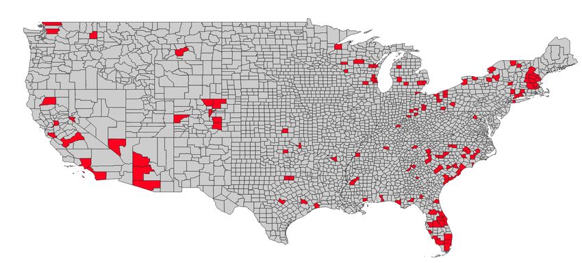
We use data on nearly 12 million traffic stops carried out by the police in the 142
counties where Trump held a campaign rally, either as a candidate for the Republican
nomination or the presidency (Figure 1).6 To measure racially-directed police behavior,
we rely on the racial classification of the motorist stopped (following, e.g., Knowles,
Persico and Todd (2001); Anwar and Fang (2006); Antonovics and Knight (2009); Anbarci
and Lee (2014); Goncalves and Mello (2021)).
To guide our empirical strategy, we outline a conceptual framework that models the
choice of a police officer to perform a traffic stop as a function of the race of the driver and
other observable characteristics of the traffic event. This model implies that the outcome
of interest consists in the probability that a traffic stop involves a Black driver (hereafter,
the probability of a Black stop). The model also illustrates the channels through which
Trump rallies can affect this outcome. We estimate the effect of Trump campaign rallies on
the probability of a Black stop using a generalized difference-in-differences methodology
(DiD) at the police stop level, controlling for county and day fixed effects as well as
county-specific time trends.7
We find evidence that Trump rallies increased the probability of a Black stop. Our
baseline estimate suggests that this probability increases by 0.94 percentage points on
average in the month following a rally, a 5.1% increase. The effect is immediate and lasts
3
Racial bias and discrimination in police behavior have been studied in several papers, including but
not limited to Antonovics and Knight (2009); Anbarci and Lee (2014); Anwar and Fang (2006); Coviello
and Persico (2015); Feigenberg and Miller (2020); Fryer (2019); Goncalves and Mello (2021); Grogger
and Ridgeway (2006); Horrace and Rohlin (2016); Knowles, Persico and Todd (2001). Prejudice against
African Americans is undoubtedly not limited to police behavior but pervades the entire justice system
and manifests in bail decisions (Arnold, Dobbie and Yang, 2018), sentencing (Depew, Eren and Mocan,
2017), parole decisions (Anwar and Fang, 2015), and capital punishment (Alesina and La Ferrara, 2014).
4
According to the Bureau of Justice Statistics, 8.6% of US residents aged 16 and over (more than
20 million people) were pulled over by the police for a traffic stop in 2015 (Davis, Whyde and Langton,
2018).
5
NPR, January 25, 2021. Several recent high-profile police killings of Black civilians followed a traffic
stop, including the shootings of Daunte Wright on April 12, 2021, and Philando Castile on July 6, 2016.
6
Typically, as described in Section 3, these rallies are large events, which gather an average of almost
5,000 people. Local police might be exposed to a rally in a given county in several ways: as security
detail or as an attendee. The presence of police officers as attendees has been widely covered in the press
(e.g., The Washington Post on 03/21/2016 or The Independent on 05/29/2016). The rallies were also
intensively covered in local media (Snyder and Yousaf, 2020).
7
Recent econometric literature on staggered difference-in-differences shows that two-way fixed effects
estimate a weighted average of each treatment effect where the weights may be negative. We first follow
the recommended diagnostics by de Chaisemartin and d’Haultfoeuille (2020) and show that none of the
weights are negative for our specification. We then follow the estimation procedure proposed by Sun and
Abraham (2018) and find similar results to our baseline DiD. We also show that our results are immune
to the recent criticism of event-study designs by Borusyak and Jaravel (2017).
3for up to 50 days. This outcome is robust to varying the observation window from 10
to 100 days around the event, as well as to including other flexible county-specific time
trends. To address the concern that the timing of rallies may be correlated with changes
in the probability of a Black stop, we first check with an event-study design that there
are no differences in pre-trends of the outcome before a Trump rally. We also show that
there are no differences in levels of the outcome just before a rally, between counties that
are about to be treated and others. Additional results show that the effects are specific
to Trump rallies. We observe no effect on police behavior of campaign events carried out
by either the Democratic contender to the presidency, Hillary Clinton, or by the other
leading Republican opponent, Ted Cruz.
Our conceptual framework highlights how the change in the probability of a Black stop
after a Trump rally could be due to a change in individual officer racial bias, patrolling
decisions, or driver behavior. We find no evidence for a change in driver behavior (either
of Black or non-Black drivers). We also observe no change in the total number of traffic
stops nor in the individual probabilities that a traffic stop is of a White driver, a Hispanic
driver, or an Asian/Pacific Islander driver.8
The change in patrolling decisions itself could stem from changes at different levels of
the hierarchy. It may come from individual officers changing their behavior, law enforce-
ment agencies changing patrolling decisions, or from local politicians imposing changes
on the police. We show that our effect is robust to controlling for officer-level fixed ef-
fects, implying that at least part of the effect is due to a change in individual officers’
behavior rather than a shift in the composition of the police force on duty. The result is
also robust to including fixed effects for each hour of the day by county, which account
for a potential change in the timing of patrols. Last, our results hold when we restrict
our sample to state troopers, which are less influenced by local politics. We conclude
that change in patrolling decisions at the enforcement agency level cannot fully explain
the effect of Trump rallies on the probability of a Black stop. Finally, we construct mea-
sures of racial bias at the individual police officer level, based on the difference in officers’
ticketing decisions towards White vs. Black drivers, controlling for a detailed set of fixed
effects that reduce heterogeneity in the context of a traffic stop. We show that this index
of officer racial bias increases after a rally.
To rationalize our findings of an effect of Trump rallies on policing behavior and racial
bias towards Black people even though Trump’s speeches never explicitly targeted that
group, we refer to a political science and law literature that shows how certain speech
carries a hidden message only understood by a subgroup – a phenomenon known as the
8
This also rules out that our main effect is due to a change in misreporting, with stops that were
previously misreported as White now reported as Black. For this to be the case, we should observe a
similarly sized decrease in the probability that a stopped driver is White, which is not the case. We
should also observe a one-to-one substitution for each category of offense, which again is not the case.
4“dog-whistle effect” (Lohrey, 2006; Fear, 2007; Goodin, 2008; Haney-Lopez, 2014).9 Dog-
whistling has been defined in various ways. Here, we consider a specific dimension of the
definition: when coded language triggers strongly rooted stereotypes about groups per-
ceived as threatening (Haney-Lopez, 2014).10 Specifically, we explore whether Trump’s
campaign activated prejudice against Black people, namely the stereotype associating
them with violence and crime (Eberhardt et al., 2004), and particularly amongst indi-
viduals with deep-seated bias against Black people. To do this, we proceed in three
steps.11
First, consistent with the argument that dog-whistling harnesses deep-rooted stereo-
types about the perceived threat of certain groups, we show that the effect of Trump
campaigns on police behavior is larger in magnitude among officers who are more biased
towards Black drivers and in areas with a stronger and deeper-seated anti-Black senti-
ment. The effect is three times as large for officers whose bias at baseline is one standard
deviation higher than the mean. There is no effect of Trump rallies on officers with
average bias. To measure the strength of local anti-Black views, we use county-average
responses to racial resentment questions included in the 2012 and 2014 Cooperative Con-
gressional Election Surveys (Schaffner and Ansolabehere, 2015). In addition, we use
proxies of deep-seated racial animus inherited from the pre-Civil War era. We follow
Acharya, Blackwell and Sen (2016) who show how the prevalence of slavery shaped racial
prejudice against Black people in the US and continues to do so to this day. Specifically,
we use the number of slaves in the year 1860 and, to deal with the potential endogeneity
of slavery, like Acharya, Blackwell and Sen (2016), and Masera and Rosenberg (2020),
we use cotton suitability as an exogenous predictor of slavery. Last, we use private and
institutional racial violence measures in the Jim Crow era: the intensity of lynchings and
9
The term dog-whistle was first coined in the context of Australian politics in the mid-1990s when the
then leader of the conservative Liberal party John Howard was accused of pandering to racist views with
coded language enabling him to maintain plausible deniability and avoid overtly racist wording (Lohrey,
2006; Fear, 2007; Goodin, 2008). Haney-Lopez (2014) describes dog-whistle techniques in American
politics in detail.
10
There is a large literature in political science and social psychology that studies the role of racial
priming on voting preferences (see e.g. Mendelberg (2008); Hopkins (2019)). Dog-whistling can be
understood as a form of implicit racial priming. It uses coded language that does not directly refer
to the targeted racial group but is understood differently by different audiences as a function of their
underlying prejudice against that racial group. It typically achieves this by exploiting common knowledge
between the principal and part of the audience or by harnessing stereotypes that are only held by part
of the audience. The theoretical persuasion literature shows how persuaders can do better in front of a
heterogeneous audience by sending private signals (Krähmer, 2020; Zhu, 2017). However, when restricted
to public communication, the principal will generally achieve a pooling, compromising action (Bar-Isaac
and Deb, 2014). Dog-whistling can thus be interpreted as a case in which the principal achieves private
communication through a public signal interpreted differently by different audiences.
11
Recently, scholars have argued that Trump has moved beyond dog-whistling by breaking racial
discourse norms and making explicit and direct racial appeals (see, e.g., Smith (2020)). While this paper
does not debate the extent to which Trump’s discourse on race is implicit or explicit, we do observe
that explicitly negative language in the 2015-2016 campaign that we study in this paper has primarily
targeted migrants rather than Black people. See Footnote 2.
5executions of Black people at the county level (Hines and Steelwater, 2012; Espy and
Smykla, 2016). We find that Trump’s campaign rallies have a significantly larger effect
in counties that today have more intense racial resentment, those that had more slaves in
1860 and whose agricultural endowments were more suitable to slavery, as well as those
where the intensities of lynching and executions of Black people were higher.12 In con-
trast to racial attitudes, other potential sources of heterogeneity such as average income,
college education, racial fragmentation, average Democrat vote share, or sheriff politi-
cal affiliation play no role in aggravating the effect of a Trump rally on police behavior.
We similarly observe no differential effect either across counties more or less affected by
import competition with China (Autor, Dorn and Hanson, 2013).
Second, we provide a direct test of a dog-whistle effect that operates beyond police
behavior and concerns the population as a whole. To do so, we revisit the experiment con-
ducted by Newman et al. (2020). This experiment took place during the 2016 Presiden-
tial campaign and presented respondents with Trump’s and other candidates’ campaign
speeches on immigration as well as other topics. While the original paper by Newman
et al. (2020) focused solely on the acceptance of discrimination against Latinos, the au-
thors also collected data on prejudice against Black people. We use the latter, to the best
of our knowledge for the first time, in this paper. Employing their sample and data, we
show that respondents with above median (or above mean) pre-existing prejudice against
Black people become even more prejudiced when exposed to Trump’s anti-immigration
rhetoric, specifically when he accused Mexican migrants of bringing drugs and crime and
of being rapists.13 No effect is observed for respondents who were not initially prejudiced
before reading Trump’s statement; nor for respondents who are exposed to speeches by
other politicians, even on the same topic of immigration, but which do not contain dog-
whistles. Moreover, the effect is specific to prejudice against Black people: no effect is
observed for bias against other groups, even for respondents who were initially prejudiced
against these groups. Consistent with the theoretical conceptualization of dog-whistling
appealing particularly to the stereotype of a threatening and dangerous group, the effect
here is also specific to a distinct dimension of prejudice: the belief that Black people are
violent, as opposed to other dimensions of bias measured in the experiment, for example,
the belief that they are lazy, or lack intelligence. We take these findings as evidence that
Trump’s rhetoric resonates, especially among individuals already prone to thinking that
Black people are violent, and radicalizes these views even further.
Third, to provide further evidence of a dog-whistle effect, we utilize the content of the
12
While the effect on the probability of a Black stop is higher, we do not observe that Trump holds
more rallies in these counties.
13
During his presidential announcement speech on June 16, 2015, Trump remarked: “When Mexico
sends its people, they’re not sending their best [...] They’re sending people that have lots of problems,
and they’re bringing those problems with them. They’re bringing drugs. They’re bringing crime. They’re
rapists.”
6speeches by Trump during his rallies in conjunction with the police data and examine
how the words included in the experimental inflammatory statement mediate the effect
of a rally on police behavior. As predicted by dog-whistling theory, and consistent with
what we find in the online sample of respondents, we find that the most prejudiced
officers are particularly triggered by those words.14 By contrast, there is no aggravating
effect on prejudiced officers of speech related to the economy, international trade, political
corruption, or Hillary Clinton.
Overall, our results show how Trump’s rallies have fueled racist behavior and sentiment
against Black people. Moreover, the experimental findings and analysis of speech content
demonstrate that it is a particular dimension of prejudice that is affected – the stereotype
that Black people are violent – thus suggesting more than a simple activation of indis-
criminate racial bigotry. Our analysis cannot, however, fully untangle whether Trump’s
rhetoric aggravated prejudice or simply activated or normalized pre-existing prejudice.
Regardless, we are able to highlight the direct and real consequences not only on views
expressed by the population but also in terms of racially-directed behavior by the police.
Moreover, since the effect is stronger in more racist areas and amongst most biased in-
dividuals, our results indicate a radicalization of prejudice against Black people, which
also contributes to polarization on racial issues. These findings are of significant policy
relevance in the United States and beyond, where politicians increasingly use xenophobic
and racist rhetoric, either explicitly or using coded language that appeals to deep-seated
stereotypes.15 Arguably, dog-whistle politics can be a powerful political tool for politi-
cians that want to engage with the more racist part of the electorate while maintaining
a veneer of plausible deniability.
Our findings contribute to an emerging literature, namely by Bursztyn, Egorov and
Fiorin (2020), Edwards and Rushin (2019), Müller and Schwarz (2019), and Newman
et al. (2020), that shows how Trump’s campaign, election, and social media activism
have unraveled social norms around the acceptability of discrimination and xenophobia.16
In contrast to this literature, we show how Trump’s campaign has aggravated prejudice
not against the groups targeted explicitly by Trump’s racially inflammatory rhetoric but
against Black people. Comparing a panel of survey respondents between 2012 and 2016,
Hopkins (2019) find that anti-Black prejudice predicts voting intentions for Trump in
2016 to a greater extent than anti-Latino prejudice. This suggests that the radicalization
14
Guided by the experiment, we use the words: Rape, Drug, Crime, Criminal, Mexico, Mexican,
bring, send, problem as the triggering words.
15
For example, in Europe, Frans Timmermans, the first Vice President of the European Commission,
accused the Prime Minister of Hungary Viktor Orban of dog-whistling antisemitic views.
16
Feinberg, Branton and Martinez-Ebers (2019) document a correlation at the county level between
hosting a Trump’s presidential rallies and the incidence of hate crimes. The authors do not account for
the potential endogenous selection of counties in which a rally is held, nor for the influence of several
potential omitted variables. Lilley and Wheaton (2019) show that this correlation is not robust when
controlling for population size.
7of prejudice which we document in this paper may have further contributed to Trump’s
electoral success. Another notable contribution of our work with respect to the existing
literature is to document the effect of Trump’s political campaign on the behavior of the
police. In this respect, our results point to how political campaigns can lead to potential
abuses of delegated authority and state violence against specific groups of citizens.
More generally, our results illustrate how politicians can radicalize prejudice and influ-
ence racially-directed behavior by triggering ingrained stereotypes. As such, our results
speak to two related strands of literature on hidden values, or “crypto-morality,” and
on the dog-whistle effect. In fact, while a plethora of recent studies have documented
the persistence of values and norms,17 some values may remain hidden, a phenomenon
described as “crypto-morality” by Greif and Tadelis (2010).18 In the context of the US,
racial inequality was the dominant accepted social norm into the early twentieth cen-
tury,19 until it was supplanted by a norm of racial equality in the post-Civil Rights
era (Mendelberg, 2001; Newman et al., 2020). Yet, negative racial views did not sim-
ply vanish; they are hidden and continue to shape political preferences (Hutchings and
Valentino, 2004; Mendelberg, 2008). Experimental and survey evidence suggests that
such negative racial predispositions can be activated either by racial cues (see Mendel-
berg (2008) for a meta-analysis) or by coded language and symbols: what the literature
calls dog-whistles (Valentino, Hutchings and White, 2002; Haney-Lopez, 2014; Valentino,
Neuner and Vandenbroek, 2018). Politicians can thus appeal to racial bias and activate
racial resentment.20 Our work, therefore, contributes to recent literature that explores
the ways leaders legitimize political preferences and mobilize their followers (Lenz, 2012;
Dippel and Heblich, 2018; Cagé et al., 2020), even to the point of prompting them to
perpetrate acts that signify a brutal and profound rupture with pre-existing norms of so-
cial and political acceptability (Cagé et al., 2020).21 By showing how dog-whistle politics
radicalize already-prejudiced individuals, this paper also complements studies on political
radicalization and polarization.22
17
This literature is now too voluminous to cite comprehensively. See Nunn (2012), Alesina and
Giuliano (2015), and Nunn (2020) for reviews.
18
This highlights a limitation of studies that measure norms in surveys. A potential confound is that
opinions revealed in surveys may be moderated by the social acceptability of expressing these views.
Studies on voting behavior are similarly constrained by the supply of political parties. For example,
Cantoni, Hagemeister and Westcott (2019) argue that the lack of supply of party platforms restricted
the expression of populist right-wing views in Germany. By contrast, we are able to observe actual
behavior by the police in this paper.
19
We define dominant social norm here as an “informal standard of social behavior accepted by most
members of the culture and that guides and constrains behavior”. (Mendelberg, 2001)
20
A related phenomenon is the activation of a collective memory of traumatic events. For example,
Fouka and Voth (2020), and Ochsner and Roesel (2019) show how politicians can gain political advantage
by stimulating historical resentment against former enemies (e.g., Germans in Greece, Turks in Austria).
21
A related literature shows how traditional or social media, rather than leaders, can facilitate the
coordination of xenophobic attacks (Bursztyn et al., 2019; Della Vigna et al., 2014; Yanagizawa-Drott,
2014).
22
See, e.g., Abramowitz and Saunders (2008); Gentzkow (2016); Abramowitz (2018); Gennaioli and
8Our paper is loosely related to a literature aiming at measuring racial bias in policing
and judicial decisions.23 Our conceptual framework shows that the probability of a Black
stop is the appropriate outcome variable to capture the effects of Trump rallies, which
may operate not only on officers’ racial bias but also on institutional policing decisions.
The rest of the paper is organized as follows. The next section presents the conceptual
background. Section 3 describes the data used in the analysis. Section 4 shows that the
probability of a Black stop increases after a Trump rally, and Section 5 shows that the
effect is not due to a change in driver behavior but to a change in policing. In line with
dog-whistling theory, we show in Section 6 that the effect is stronger for more biased
officers and in areas with a stronger and deeper-seated anti-Black sentiment. We provide
experimental evidence on the effect of exposure to Trump’s racially inflammatory speech
on racial prejudice in the population in Section 7. We then show how such racially
inflammatory speech also amplifies the effect of Trump rallies on traffic stops of Black
drivers in section 8. In conclusion, we discuss broader implications.
2. Conceptual Background
To motivate our empirical strategy, we introduce a simple model of traffic stop decisions
by a police officer. This model helps clarify what the outcome of interest is and how –
through which channels – it is potentially affected by Trump rallies.
In our setting, an officer j observes driving event i and has to decide whether to stop
the car. S denotes the stop decision. A driving event is characterized by the driver’s race,
Ri,j , and other observable characteristics Mi,j . The race of the driver can either be Black
(Ri,j = 1) or non-Black (Ri,j = 0) and is drawn from a Bernoulli distribution fj . The
probability that Ri,j = 1 is pj . We, therefore, allow for different officers to face a different
racial composition of drivers, for example, if they are deployed in different neighborhoods.
Mi,j includes all the characteristics of the event that impact the utility that an officer
derives from a stop, beyond race. For example, Mi,j encompasses policing objectives such
as the potential deterrence or incapacitation effect of the stop, career concerns of the
officer, or the inconvenience of the stop, such as attending traffic court. Mi,j is drawn
from a distribution gR,j where R is the race of the driver of event i. We thus allow for
drivers of different races to systematically drive differently. pj and gR,j could depend on
three factors: driver demographics and behavior, institutional patrolling decisions, and
individual officers’ patrolling decisions.
The officer derives the following utility from an event:
Tabellini (2019); Bordalo and Yang (2020) for recent contributions documenting polarization in the US.
While many, in particular, Abramowitz (2018), argue that Trump’s rise to power was the consequence
of polarization, we focus instead on how his campaign further deepened divisions.
23
See footnote 3, Lang and Kahn-Lang Spitzer (2020) for a recent review, and Arnold, Dobbie and
Yang (2018), Goncalves and Mello (2021), and Ba et al. (2021) for recent contributions.
9
0 if Si,j = 0
Ui,j (Si,j , Mi,j , Ri,j ) = (1)
M + λj Ri,j if Si,j = 1
i,j
λj parametrizes the racial bias of the officer. An officer with a positive λj derives
higher utility from stopping a Black driver compared to a non-Black driver, everything
∗
else constant. The optimal stopping strategy of officer j when faced with an event i (Si,j )
is therefore defined by:
1 if M > −λ R
∗ i,j j i,j
Si,j (Mi,j , Ri,j ) = (2)
0 if M < −λ R
i,j j i,j
This implies that an officer with higher λj will stop a Black driver for a larger set of
observable characteristics Mi,j than they would a non-Black driver.
One issue here is that we only observe Si,j = 1 in the data. This is because we do not
observe the universe of driving events, but only when a driver is stopped. We therefore
focus on the implications of the optimal stopping strategy based only on stops that are
made. In particular, we derive the probability that a stop made by officer j is of a Black
driver as:
P rob(fj = 1)P rob(g1,j ≥ −λj )
qj =
P rob(fj = 1)P rob(g1,j ≥ −λj ) + P rob(fj = 0)P rob(g0,j ≥ 0)
(3)
pj [1 − G1,j (−λj )]
=
pj [1 − G1,j (−λj )] + (1 − pj )[1 − G0,j (0)]
where GR,j is the CDF of gR,j .
The numerator of this expression is the probability that an event leads to a stop of a
Black driver. It is the product of two components: the probability that the driver is Black
and the probability that this event by a Black driver leads to a stop. The denominator
is the probability that an event leads to a stop. It is the sum of the probability that an
event leads to a stop of a Black driver and the probability that an event leads to a stop of
a non-Black driver. From now on, we will refer to qj as the probability of a Black stop.
Proposition 1. The probability of a Black stop qj increases in racial bias λj and in the
probability that the driver is Black pj . If g1,j first order dominates g1,j 0 then qj > qj 0 . If
g0,j 0 first order dominates g0,j then qj > qj 0 .
Proof: See Appendix 4.
According to the prediction of dog-whistling, we expect Trump campaign events to
increase qj through several possible channels. The first is through an increase in racial
bias λj . The second is through changes in individual or institutional patrolling decisions.
For example, qj could increase because of an increase in pj if officers patrol areas with
10more Black drivers, or because officers patrol areas where they are more likely to face an
event in which Black drivers have a high Mi,j , or non-Black drivers a low Mi,j (resulting
in a change in either G1,j or G0,j ).
Trump rallies could also increase qj through channels unrelated to dog-whistling. They
could change who drives and how. For example, Black drivers could drive more, or non-
Black drivers less, which would increase pj . Another possibility is that Black drivers
would change their driving behavior in a way that is more likely to lead to a stop (change
in G1,j ), or non-Black drivers change their driving behavior in a way that is less likely to
lead to a stop (change in G0,j ). In Section 4,we first establish that Trump rallies result
in an increase in qj . We then investigate in Section 5 the different channels behind this
effect.
3. Data
In what follows, we describe the data sources used in the paper.
Police Stops: Our data on police traffic stops comes from Pierson et al. (2020),
who have made the information publicly available on the Stanford Open Policing Project
website. To construct a national database of traffic stops, they filed public records re-
quests with all 50 state patrol agencies and over 100 municipal police departments. More
details on the data collection can be found in Pierson et al. (2020). Altogether, the data
comprises approximately 95 million stops from 21 state patrol agencies and 35 municipal
police departments from 2011-2018. We focus on the sample of stops in the years 2015-
2017 in counties where Trump held a rally during his 2015-2016 campaign. This gives us
a total of 11, 931, 161 stops for which we have information on the date of the stop and
the driver’s race. The race is recorded as “Asian/Pacific Islander”, “Black”, “Hispanic”, or
“White.” Information on the final decision made by the officer for a stop is available for
7, 521, 505 of these stops and has been coded by the Stanford Open Policing Project into
four possible categories (in increasing severity): warning, citation, summons, and arrest.
For a more limited set of stops (5, 387, 948), information is also available on the reason
why the driver was stopped.
Campaign Rallies: Data on the rallies held by the 2016 presidential candidates
comes from the Democracy in Action website (Appleman, 2019), which documents pres-
idential candidates’ schedules, from pre-campaign to presidential inauguration. We geo-
code all Donald Trump’s rallies for the 2015-2016 presidential campaign that started on
June 17, 2015 and ended on November 7, 2016. Altogether, 224 Trump campaign rallies
(out of 324) in 142 counties overlap with traffic stop data. Typically, Trump’s rallies were
large events, gathering an average of 4,774 people across 2015-2016 (with 4,930 people on
average for nomination rallies and 4,619 for presidential rallies).24 We also geo-code in-
24
From Wikipedia (2016).
11formation on the 2016 Democratic presidential candidate, Hillary Clinton, and the other
main Republican contender, Ted Cruz.
County Characteristics: Data on ethnic fractionalization, average income, the
share of Blacks, and average college completion comes from the 2015 American Commu-
nity Survey. Data on county-level import competition shock is from Autor, Dorn and
Hanson (2013), while the information on 2012 county-level vote shares for Obama comes
from Leip (2016).
Summary Statistics: Summary statistics are provided in Table 1. Black people
represent 11.22% of our sample population, but as much as 20.39% of stops. Black
drivers are thus over-represented in stops by a factor of two. 51.50% of stops are of White
drivers and 24.13% of Hispanic drivers. Black drivers represent 22.8% (6.87/30.18) of the
warnings and 17.2% (0.81/4.70) of the arrests.
In addition to the above main sources of information, we also exploit the following
county-level sources to explore heterogeneous effects:
Racial Resentment: We derive our measure of racial resentment from the 2012
and 2014 Cooperative Congressional Election Surveys (Schaffner and Ansolabehere, 2015)
(hereafter, CCES). We chose the 2012 and 2014 waves to obtain a measure of pre-existing
racial resentment before the launch of the Trump campaign. Specifically, we use questions
CC442a and CC422b, which ask respondents how much they agree, on a scale of 1 to
5, to the following statements: “The Irish, Italians, Jews and many other minorities
overcame prejudice and worked their way up. Blacks should do the same without any
special favors” (“Racial Resentment A”); ”Generations of slavery and discrimination have
created conditions that make it difficult for Blacks to work their way out of the lower class”
(“Racial Resentment B”). We calculate the share of Whites who somewhat or strongly
agree with the first statement and the share of Whites who somewhat or strongly disagree
with the second statement. Higher values, therefore, indicate greater resentment.
Responses to survey questions about racial resentment could suffer from conformity
or social desirability bias, which would bias our estimates towards zero. To circumvent
this limitation, we also use several proxies of deep-seated racial animus. As argued by
Acharya, Blackwell and Sen (2016, 2019), present-day racism in the US can be traced
back to slavery, which we proxy by the number of slaves per capita in 1860.25 To deal
with the potential endogeneity of slavery to local cultural and political factors, we use
cotton suitability as an exogenous predictor of slavery, following Acharya, Blackwell and
Sen (2016) and Masera and Rosenberg (2020). We also use measures of private and
institutional racial violence between the Civil War and World War II, which we proxy by
the local intensity of lynchings (from Hines and Steelwater (2012)) and of executions of
Blacks (from Espy and Smykla (2016)) at the county level.
25
We use the Census of 1860, the last official record of the number of slaves prior to the abolition of
slavery.
12The experimental data is described in Section 7. The data on Trump’s rallies speeches
is described in Section 8.
4. Empirical Strategy and Results
We follow our conceptual background and Equation 3 to guide our empirical strategy and
show the effect of Trump rallies on the outcome of interest: the probability of a Black
stop.
4.1 Difference-in-Differences Analysis
4.1.1 Empirical Specification We conduct our analysis at the stop level, estimating
whether a Trump campaign rally e leads to an increase in the probability that the driver
(a,b)
stopped by the police in stop i in county c on date t is Black. We first define Dc,t as
a dummy variable equal to 1 if day t is within a and b days from any event in county
c. Formally, Dc,t = Max (1(a ≤ dc,t,e ≤ b)e=1,...,Nc ), where dc,t,e is the distance (in days)
(a,b)
of day t from Trump rally e in county c. dc,t,e is positive if day t is after the event and
negative if day t is before the event. A given county can have more than one event, and
up to Nc events. Out of the 142 counties in our sample, 99 have exactly one Trump rally,
(−∞,a)
while 23 have 3 or more rallies. With a slight abuse of notation, Dc,t is defined as a
dummy variable equal to 1 if the distance of day t from any Trump rally in county c is less
(a,∞)
than a. Similarly, Dc,t is a dummy variable equal to 1 if the distance of day t from any
= Max (1(dc,t,e ≤ a)e=1,...,Nc )
(−∞,a)
Trump rally in county c is more than a. Formally, Dc,t
and Dc,t = Max (1(dc,t,e ≥ a)e=1,...,Nc ).
(a,∞)
Our estimation equation is:
(−∞,−k−1) (0,0) (1,k) (k+1,∞)
Black i,c,t = αc + θt + γDc,t + ηDc,t + βDc,t + δDc,t + αc × t + ui,c,t , (4)
where Black i,c,t is a dummy that takes value one if the driver pulled over by the police in
stop i in county c on date t is Black. In terms of our conceptual framework, we estimate
changes in the average qj in county c on date t after a Trump rally.
One concern may be that counties in which Trump held a rally differ systematically
from other counties. For example, Trump or his campaign team might target counties as
a function of their underlying racism or police behavior. Time-invariant county institu-
tional or cultural characteristics, including racism, permanent police capacity, legislative
differences, or geographic differences, are captured by county fixed effects αc . Addition-
ally, to account for county-specific time trends in the probability of a Black stop, we
include county-specific linear time trends αc × t. To address potential remaining issues
related to the systematic selection of counties with a campaign event, we rely only on
the set of counties in which Trump has ever held a rally in the estimation of Equation
134 (although our results are robust to including never-treated counties). Day fixed effects
θt account for daily fluctuations in the nature of the traffic stops; for instance, across
different days of the week, holidays, or end of the month effects. We focus our analysis
on police stops in the years 2015-2017.
A rally may disrupt the daily routine of police departments in several ways. On the
one hand, the organization of a large-scale public event could mean that police officers
are deployed near the venue of the rally and are not patrolling the roads as they usually
do. On the other hand, the authorities may prefer to enhance security in their local area
by increased patrolling of roads. We control for such disruptions using an indicator that
(0,0)
takes the value of one for county c on date t of the day of the rally (i.e., for Dc,t ).
Our main parameter of interest is β. The variable that captures the treatment is a
dummy variable that takes the value of one for the k days following any Trump rally in
that county and zero otherwise.
To address potential concerns about the selection of the treatment window, we adopt
a flexible approach. Specifically, we estimate Equation 4 varying the time window k after
a Trump rally by increments of 10 days, from 10 to 100 days. The omitted comparison
time window consists of an identical window (k = −10 , ..., −100 , i.e., 10 to 100 days
(−∞,−k−1)
before the rally), immediately prior to the rally. We therefore control for Dc,t ,
(k+1,∞)
which is equal to one for the days prior to the comparison window k, and Dc,t , which
is equal to one for the days following our treatment period. For counties with multiple
events, we allocate each stop i in county c to each possible event in the county and define
the windows around each event.
To define the dummy variables that capture the different windows, it is thus necessary
to take the maximum of the indicator variables that capture the possible windows for each
possible event. For example, if we consider a treatment window k of 30 days after a rally,
the omitted comparison window is 30 days before the rally (for all possible rallies in the
(−∞,−31) (31,∞)
county), Dc,t indicates more than 30 days before a rally and Dc,t more than 30
days after the rally. β, therefore, captures the change within a county in the probability
of a Black stop 30 days after any Trump rally compared to the 30 days prior.
In the potential outcome framework, our identification assumption requires that after
controlling for day fixed effects and county-specific linear trends, the probability of a
Black stop would not change in the k days after a Trump rally compared to k days
before, in the absence of the rally. This assumption would be violated if Trump rallies
were systematically timed to correspond with an increase in the probability of a Black
stop. We address this in four ways. First, we include county-specific time trends. Second,
we show in Table A1 that there is no statistically significant difference in the probability
of a Black stop just before a rally between counties that are about to be treated and other
counties. We show this for alternative windows of 5, 10, or 30 calendar days before the
rally in order to capture reasonable time frames for the scheduling of rallies. Third, in
14Section 4.2, we present the findings of an event-study analysis that shows the absence of
pre-trends in the probability of Black stops across counties. The event study results also
show that the only period in which we pick up a treatment effect is immediately after a
Trump rally and that the effect lasts up to 50 days. Last, results of permutation inference
(based on 1, 000 replications) in which we randomly reassign Trump rallies within counties
across days show that our effect size is well outside the range of estimated effects from
these placebo treatments (see Figure A2).26
A potential threat to correct inference on the treatment effect consists of the serial
correlation of the error term uict within a county over time or across counties on a partic-
ular date. We consequently adjust standard errors for two-way clustering at the county
and day level. In Section 4.1.2, we check that our results are not subject to potential
issues with the two-way fixed effects estimators highlighted by Sun and Abraham (2018),
de Chaisemartin and d’Haultfoeuille (2020), and Borusyak and Jaravel (2017).
4.1.2 Results Table 2 shows the estimates of Equation 4 for increasing windows k
around a Trump rally. We observe that the probability of a Black stop increases after a
Trump rally. The effect is immediate, constant in magnitude for the first 30 days after
a rally, and then slowly fades away. The effect remains statistically significant for up
to 100 days after a rally, although at the 100-day window, it is only half in magnitude
compared to the largest effects immediately after the rally, suggesting that the effect lasts
for around 50 days. An event-study analysis will confirm that the effect is very stable in
the first month after a rally, largest in magnitude for up to 30 days, then declines and is
no longer significant 50 days after the rally. In what follows, we retain a 30-day window
after a rally as the main focus of our analysis.
In Table A2, we verify that our results are robust to excluding county specific time
trends or instead to including county-specific quadratic time trends (Columns 1 and 2).
Borusyak and Jaravel (2017) show that in some settings with staggered treatment where
each unit is treated only once, econometric models with unit and time fixed effects are un-
able to identify a unit-specific linear trend. This happens in fully dynamic settings where
the treatment effect persists even after the estimation sample ends. In these settings, the
authors recommend dropping the linear trend or including never-treated observations.
Our analysis is unlikely to suffer from this issue as the treatment effects last for only 50
days and our estimation sample includes many days after that. We nonetheless follow
their recommendations and show in Table A2 that our results are robust to dropping the
26
It is not unexpected that the distribution of the estimated placebo treatment effects has more
extreme positive values compared with negative values in the presence of a dynamic treatment effect
that fades over time and when the treatment effect is estimated using a sharp window, such as in our
setting. If the placebo treatment date falls close to the actual treatment date, the estimated placebo effect
will take an extreme positive value (close to the true treatment effect), which will not be compensated by
similarly high negative treatment effects when the placebo treatment falls further away from the actual
treatment.
15linear trend (Column 1) and to including never-treated units (Column 3). We consider as
never-treated units the counties where other major political candidates in the 2015-2016
campaign (Clinton or Cruz), but not Trump, held a rally. We do so in order to reduce
the potential heterogeneity between treated and untreated counties. When we include
those counties, adding about 5 million observations to the estimation sample, the esti-
mated coefficient becomes larger in magnitude (from 0.94 to 1.01) and still statistically
significant at the 1% level.
Recent econometric literature on staggered difference-in-differences highlights poten-
tial issues with the two-way fixed effect estimator employed here. One of the main insights
of this work is that the estimated parameter is a weighted average of each treatment (in
our context, each rally) where the weights may be negative. We consequently follow
the recommended diagnostics by de Chaisemartin and d’Haultfoeuille (2020). Figure A3
shows that there is little variation in the weights and that none is negative in our pre-
ferred specification with k = 30 days after a rally. However, our setting does not perfectly
match the situations studied by de Chaisemartin and d’Haultfoeuille (2020). First, the
treatment only lasts for up to 50 days. Second, a county may be treated multiple times.
Third, we bin days together to estimate the average effect of a Trump rally in the first k
days (with k = 30 in our preferred specification). In a context more similar to our own,
Sun and Abraham (2018) propose estimating the treatment effect for each event and then
averaging the event-specific treatment effects out. Figure A4 displays the distribution of
the estimated difference-in-differences parameters for each county. Following their tech-
nique, we combine these estimates (with equal weights) and find that the probability of
a Black stop increases from 0.94 p.p. in our baseline to 0.98 p.p., suggesting that our
baseline estimate is, if anything, underestimated.
We show that our results are robust to alternative measures of the dependent variable
(logarithm or inverse hyperbolic sine of the share of Black stops in a county-day) in
Columns 4 and 5 of Table A2). Last, in Section 2.3 of the Appendix and Table A3, we
show that our results are robust in an alternative difference-in-differences specification,
in which we fix the pre-treatment window to 100 days and only include observations k
days after a rally, for k = 10, ..., 100.
In terms of magnitude, we estimate a 0.94 p.p. increase in the probability of a Black
stop during the first 30 days following a Trump campaign rally. Given that in our es-
timation sample, the probability of a Black stop in the 30 days before a Trump rally
is 18.65%, this estimate amounts to a 5.1% increase. The total number of stops in our
sample in a 30-day window prior to any rally is 575,042. Thus, our analysis reveals that
Trump’s rallies led to 5,470 additional stops of Black people by the police in the month
following the events. Note that this number is an underestimate since we only have in-
formation on 224 out of the roughly 320 campaign rallies and on a subset of days and of
law enforcement agencies.
16To estimate the overall effect of the 2015-2016 Trump campaign, notice that the
police makes about 55,000 stops a day overall (Davis, Whyde and Langton, 2018). In
our sample, the average rally is held in a county with a population of 785,338 or around
0.243% of the total US population. We can use this information to produce a back-
of-the-envelope calculation of the overall effect of the Trump 2015-2016 campaign by
making some simplifying assumptions. First, let us assume that our sample of rallies is
representative of the overall population of Trump rallies. Second, let us assume that,
on average, police stops are similarly distributed between counties that hold and do not
hold Trump rallies. Given these assumptions, police in a county that holds a Trump
rally perform 134 stops a day (0.243% of 55,000). This suggests that if we were able
to observe all the stops in all the counties in which Trump ever held a rally, we would
observe 1, 286, 400 (calculated as 134 stops × 320 rallies × 30 days) stops in a 30-day
window before any rally, and not 575, 042 as in our sample. Our estimates, therefore,
imply that Trump’s rallies led to 12,237 additional stops of Black drivers by the police in
the 30 days following the rallies and 17,409 stops of Black drivers in the 50 days following
the rallies.27
Our analysis thus far considers all the rallies held during the campaign, both those
for the nomination and those for the presidency. Yet, some of the rallies held for the
nomination occurred when Trump was still a marginal player. We may thus expect that
the rallies held during his presidential campaign had bigger effects. Indeed, the increase
in Trump’s visibility and popularity, from when he became the Republican nominee and
throughout his presidential campaign, may have had an emboldening effect. For example,
the experiment by Bursztyn, Egorov and Fiorin (2020) reveals that signals of Trump’s
popularity make xenophobic respondents more likely to express their views against im-
migrants. That said, Enke (2020) shows that Trump’s campaign became more moderate
after he secured the Republican nomination, which would instead imply that the presi-
dential rallies had a smaller effect.28 In column 6 of Table A2, we differentiate between
rallies held either before or during the presidential campaign. We find that consistent
with the moderation of speech over the course of the campaign described by Enke (2020),
the effects are significantly smaller for general election rallies.
A potential concern is that Black i,c,t may be mismeasured and that Trump rallies
27
The effect in the 30 days after a Trump rally is computed as 5, 470 (additional stops of Black people
in the month following a rally) × 1, 286, 400 (the number of total stops we would observe in a 30-day
window before any rally if we observed all rallies and all police agencies) ÷ 575, 042 (the number of stops
we actually observe in a 30-day window prior to any rally). We follow the same steps using coefficient
estimates for a 50-day window to estimate the effect in the 50 days after a Trump rally.
28
It is also possible that places visited during the nomination campaign were very different from
places visited during the presidential campaign. Additional analysis in Appendix Table A4 suggests,
however, that the counties in which Trump held campaign rallies for the Republican nomination did
not statistically differ from counties in which he held rallies for the general election along a wide range
of dimensions, including pre-trends in the number of police stops or the share of stops involving Black
drivers.
17systematically affects this mismeasurement. Recent literature shows that police may
misclassify the race of stopped drivers. For example, Luh (2019) shows that minority
drivers are sometimes misreported as Whites. Misclassification could affect the validity of
our results if the misreporting of Blacks as Whites systematically decreases after a Trump
rally. If this was the case, we should observe a decrease in the probability that a stopped
driver is White of the same magnitude as the increase for Blacks. To check for this, we
report in Column 5 of Table 4 estimates of Equation 4 where the outcome is a dummy
variable equal to one if the stop is of a White driver. The coefficient associated with
the post-Trump rally dummy is not statistically significant, suggesting that systematic
changes in misclassification cannot explain our result.
To better illustrate the dynamics of the effect, we now turn to an event-study analysis.
4.2 Event-study Analysis
In this section, we perform an event-study analysis, which offers several advantages. First,
it allows to check for the existence of trends in our dependent variable before a Trump
rally, and after our treatment window. Second, it enables us to estimate precisely when
the effect of a Trump rally materializes. Third, we can study how the effect changes,
across each time period, rather than averaging over the whole window k as we did before.
The event-study specification is as follows:
(−∞,−106)
X (τ,τ +14)
Black i,c,t = αc + θt + γDc,t + βτ Dc,t
τ =−105(15)−30
(0,0)
X (τ,τ +14) (106,∞)
(5)
+ β0 Dc,t + βτ Dc,t + δDc,t + αc × t + ui,c,t
τ =1(15)91
To smooth out noise in daily observations, we estimate parameters for a 15-day win-
(τ,τ +14)
dow. Dc,t is equal to one for county-day observations that are between τ and τ + 14
(−∞,−106)
days from a Trump rally. Dc,t is equal to one for county-day observations that are
(106,∞)
more than 105 days before a rally. Dc,t is equal to one for county-day observations
that are more than 105 days after a rally. In all specifications, we include county and day
fixed effects as well as county-specific time trends. In this event study, the omitted time
(−15,−1)
bin is Dc,t , which identifies the 15 days prior to a Trump rally.
Figure 2 shows the estimates of βτ in Equation 5. We see that Trump rallies result in
a substantial and immediate spike in Black traffic stops following a rally. The probability
of a Black stop increases by 0.8 p.p. in the first 15 days after a rally. It remains stable
for 30 days after a rally and reaches its highest magnitude at that point. The effect is
nevertheless transitory and has faded away by 60 days after a rally. The figure also shows
the trend in the probability of a Black stop prior to a Trump rally, which is very stable
and does not change significantly in either direction up to 105 days leading up to a rally.
This result suggests that Trump did not specifically time his rallies in certain counties as
18You can also read