Volatility Spillovers among Developed and Developing Countries: The Global Foreign Exchange Markets - MDPI
←
→
Page content transcription
If your browser does not render page correctly, please read the page content below
Journal of
               Risk and Financial
               Management

Article
Volatility Spillovers among Developed and Developing
Countries: The Global Foreign Exchange Markets
Walid Abass Mohammed

                                          College of Business, Technology and Engineering, Sheffield Hallam University, Sheffield S1 1WB, UK;
                                          w.mohammed@shu.ac.uk

                                          Abstract: In this paper, we investigate the “static and dynamic” return and volatility spillovers’
                                          transmission across developed and developing countries. Quoted against the US dollar, we study
                                          twenty-three global currencies over the time period 2005–2016. Focusing on the spillover index
                                          methodology, the generalised VAR framework is employed. Our findings indicate no evidence of
                                          bi-directional return and volatility spillovers between developed and developing countries. However,
                                          unidirectional volatility spillovers from developed to developing countries are highlighted. Fur-
                                          thermore, our findings document significant bi-directional volatility spillovers within the European
                                          region (Eurozone and non-Eurozone currencies) with the British pound sterling (GBP) and the Euro
                                          (EUR) as the most significant transmitters of volatility. The findings reiterate the prominence of
                                          volatility spillovers to financial regulators.

                                          Keywords: foreign exchange market; volatility spillover; return spillover; VAR framework; variance
                                          decomposition; financial crisis; financial interdependence


                                          JEL Classification: G01; G1; F3
Citation: Mohammed, Walid Abass.
2021. Volatility Spillovers among
Developed and Developing
Countries: The Global Foreign
                                          1. Introduction
Exchange Markets. Journal of Risk and
Financial Management 14: 270.                   The increasing financial interdependence, particularly during the current era of global
https://doi.org/10.3390/jrfm14060270      economic events and financial turbulence has prompted considerable interest from market
                                          participants and academic research. While much attention has been paid to the magni-
Academic Editor: Edoardo Otranto          tude of return and volatility spillovers across global stock markets, little is known about
                                          the foreign exchange channels, in particular, the foreign exchange markets’ channels
Received: 3 May 2021                      between developed and developing countries. Some studies of this kind have inves-
Accepted: 7 June 2021                     tigated the return co-movements and volatility spillovers, primarily across the devel-
Published: 16 June 2021                   oped countries Andersen et al. (2001), Pérez-Rodríguez (2006), Boero et al. (2011), and
                                          Rajhans and Jain (2015). Others have considered the regional spillover transmission and
Publisher’s Note: MDPI stays neutral      produced insignificant results.
with regard to jurisdictional claims in         However, given the trillions of dollars of exchange rate trading in international fi-
published maps and institutional affil-   nancial markets, it is important to fully understand and investigate in greater depth the
iations.                                  potential spillovers of international currencies. This is an important aspect that investors
                                          must account for during the formation of their position and portfolios. Before the recent
                                          financial turmoil, the contribution of the channels of foreign exchange markets’ spillovers
                                          to the global financial instability, for some, appeared to be less worrisome. Whereas in
Copyright: © 2021 by the author.          fact, the behaviour of the stock prices (which have been extensively studied) is mainly
Licensee MDPI, Basel, Switzerland.        explained by volatilities in the foreign exchange markets Kim (2003).
This article is an open access article          Thus, in this paper, we provide new insights into the incomplete investigation of
distributed under the terms and           the channels of global intra-foreign exchange markets’ spillovers. Our key question is
conditions of the Creative Commons        whether the effect of return and volatility spillovers is bidirectional between developed
Attribution (CC BY) license (https://     and developing countries. This is because of the recent financial crisis which originated
creativecommons.org/licenses/by/
                                          in major financial hubs in developed countries, primarily in the USA, that developing
4.0/).

J. Risk Financial Manag. 2021, 14, 270. https://doi.org/10.3390/jrfm14060270                                    https://www.mdpi.com/journal/jrfm
J. Risk Financial Manag. 2021, 14, 270                                                                                             2 of 30

                                         countries are not responsible for, nevertheless, are seriously affected by it. To study the
                                         return and volatility spillovers’ transmission, we model the daily spot exchange rates for
                                         23 global currencies. According to the BIS (2013), the USD, EUR, GBP, AUD, CAD, JPY, and
                                         CHF are the most traded globally and account for almost 90 per cent of the global foreign
                                         exchange turnover. In particular, we adopt the generalised vector autoregressive (VAR)
                                         approach focusing on the variance decomposition of Diebold and Yilmaz (2009).
                                               The innovative feature of this approach, in addition to being rigorous, is that it allows
                                         the aggregation of valuable information across markets into a single spillover index. The
                                         unique structure of the spillover index is designed to unleash an in-depth analysis of the
                                         negative spillovers’ transmission across markets, i.e., how a shock in a particular market is
                                         due to exogenous/endogenous shocks to other markets.
                                               Financial crises are almost difficult to predict; nevertheless, it is important to identify
                                         fluctuations in volatility over a different time period. Thus, we examine the time-varying
                                         net volatility spillovers using the autoregressive conditional heteroskedasticity (ARCH)
                                         model. The time-varying volatility identifies the specific points of significant shifts in
                                         volatility spillovers during the time period of our sample (2005–2016). We provide evidence
                                         of significant volatility clustering during the 2008 financial crisis. The ARCH model, which
                                         was first introduced by Engle (1982) is widely used in the literature Bollerslev et al. (1994),
                                         Kaur (2004), Basher et al. (2007) for its ability to capture persistence in time-varying
                                         volatility based on squared returns. Most importantly, to investigate the nature of the
                                         net volatility and net pairwise spillover effects, we implement Diebold and Yilmaz (2012)
                                         methodology. By doing so, we are able to show the difference between the amount of
                                         the gross volatility shocks within our sample that were transmitted to and received from
                                         developed and developing countries. To enhance the reliability of the findings, we provide
                                         evidence in different dimensions (using a sample of twenty-three global currencies over the
                                         time period 2005–2016). The first is the static analysis approach, which provides results in
                                         the form of spillover tables. The second is the dynamic analysis, which yields the spillover
                                         plots. Third, is the time-varying net volatility results, which we provide in the form of
                                         figures. Finally, the net volatility and net pairwise spillover effects.
                                               The analysis is based on a large daily spot exchange rates’ dataset, which covers a
                                         long period pre and post the most recent events in the global economy. In particular, in
                                         this paper, we provide results based on extensive empirical analyses, such as the spillover
                                         index (both static and dynamic analyses), time-varying net volatility, net volatility, and net
                                         pairwise volatility effects.
                                               Guided by the empirical approach described above, the main findings indicate that
                                         there is no evidence of bidirectional volatility spillovers between developed and develop-
                                         ing countries. Although unsurprisingly, the results highlight evidence of unidirectional
                                         volatility spillovers pouring from developed to developing countries. In particular, the
                                         volatility spillovers from developed to developing countries seemed to be specifically
                                         strong following the collapse of Lehman Brothers in 2008. Another curious outcome of the
                                         findings is that developed countries are the highest receivers and transmitters of volatility
                                         spillovers, dominated by the British pound sterling, the Australian dollar, and the Euro,
                                         whereas developing countries are net receivers of volatility spillovers. The findings, there-
                                         fore, indicate that the currency crisis tends to be regional Glick and K. Rose (1998) and
                                         Yarovaya et al. (2016).
                                               Meanwhile, in light of the recent financial crisis, the analytical results demonstrate that
                                         the cross-country spillover activities between developed and developing countries are in-
                                         significant. Although the financial risk propagated during the 2008 financial crisis engulfed
                                         the global economy, that being said, because of the recent financial markets’ developments,
                                         such as financial engineering (collateral debt obligation, credit default swap, and derivative
                                         securities), financial risks triggered different means of spreading across the global economy,
                                         which still need to be discovered, understood, and described appropriately.
                                               The remainder of this paper is organised as follows: In Section 2, we discuss some
                                         critical arguments presented in the related literature; in Sections 3 and 4, we introduce the
J. Risk Financial Manag. 2021, 14, 270                                                                                             3 of 30

                                         data used in the analysis and the empirical methodology applied; in Section 5, we provide
                                         empirical results, including the robustness and some descriptive statistics; in Section 6, we
                                         discuss the time-varying volatility; in Section 7, we introduce the net spillovers and net
                                         pairwise volatility spillovers; in Section 8, we provide conclusions; and in Section 9, we
                                         discuss the study limitations and future research.

                                         2. Related Literature
                                               This brief review of the literature is focused on the foreign exchange markets’ spillover
                                         channels, which is one of the most intensely debated issues in recent literature. However,
                                         the significance of the foreign exchange markets’ spillover channels to the stability of
                                         financial markets was acknowledged three decades ago. For example, Engle III et al. (1988)
                                         established the first thread-tying efforts of the intra-day exchange rate’s volatility spillovers
                                         within one country (heat waves) and across borders (meteor shower). The “heat waves” is
                                         a hypothesis that indicates that volatility in one market may continue in the same market
                                         the next day, whereas the “meteor shower” is a phenomenon, which implies that volatility
                                         in one market may spillover to another market.
                                               In this paper, the authors provide evidence of transmitted volatility spillover from
                                         one market to another. This opening up, particularly after the 2008 financial crisis, am-
                                         plified the importance of the spillover channels in the stock and the foreign exchange
                                         markets. This is due to the repercussions of the shocking types of financial risks stem-
                                         ming from the interconnected nature of the financial markets. Thus, there is a shred of
                                         growing evidence in the literature that supports the association of return and volatility
                                         spillovers with global economic events and financial crises (for reviews see Diebold and Yilmaz
                                         (2009), Beirne et al. (2013), Yilmaz (2009), Gebka (2012), Jung and Maderitsch (2014), Ghosh
                                         (2014), Choudhry and Jayasekera (2014), Antonakakis et al. (2015), Mozumder et al. (2015)).
                                         In addition, the recent financial crisis demonstrates the severity of the cross-market volatility
                                         spillovers, which transmitted across countries through the stock and foreign exchange mar-
                                         kets’ channels (for reviews see Fedorova and Saleem (2009), Cecchetti et al. (2011), Awartani
                                         and Maghyereh (2013), Jouini (2013), Shinagawa (2014), Do et al. (2015)). Another important
                                         feature of the foreign exchange spillover channels is that their effects act differently during,
                                         before, and after the economic events and financial crisis episodes. For example, based on
                                         VAR models, Diebold and Yilmaz (2009) examined nineteen global equity markets from
                                         the 1990s to 2009. They found striking evidence that return spillovers displayed a slightly
                                         increasing trend but no bursts, while volatility spillovers displayed no trend but strong bursts
                                         associated with crisis events.
                                               In addition, the effect of return and volatility spillovers may extend to the busi-
                                         ness cycle mechanism. Several studies Imbs (2004), Eickmeier (2007), Imbs (2010), and
                                         Claessens et al. (2012) have argued that volatility spillovers inflicted business cycle syn-
                                         chronisation between countries through different channels. These channels mainly include
                                         the exchange rate, confidence, trade, and financial integration channel. Antonakakis et al.
                                         (2015) suggested that the spillover effect could also be transmitted through business cycles
                                         across countries. According to Eickmeier (2007), the confidence channel represented the
                                         response from domestic agents to the potential spillovers coming from foreign shocks to
                                         the local economy.
                                               Several studies have attempted to empirically analyse the exchange rate co-movements
                                         and volatility spillovers across countries, in particular, the financial transmission between
                                         the Euro (EUR), British pound sterling (GBP), Australian dollar (AUD), Swiss franc (CHF),
                                         and the Japanese yen vis-à-vis the US dollar. For instance, Boero et al. (2011) and Rajhans
                                         and Jain (2015) found a high correlation between the Euro and the British pound sterling
                                         against the US dollar and that the British pound sterling was a net receiver. Nikkinen et al.
                                         (2006) studied the future expected volatility linkages among major European currencies
                                         (the Euro, the British pound sterling, and the Swiss franc) against the US dollar. They
                                         found future volatility linkages between the major currencies and that the British pound
                                         sterling and the Swiss franc were significantly affected by the implied volatility of the Euro.
J. Risk Financial Manag. 2021, 14, 270                                                                                          4 of 30

                                         Boero et al. (2011) found an increase in co-movements between the Euro and the British
                                         pound sterling after the introduction of the Euro as compared with the pre-euro era. A
                                         different perspective was offered by Antonakakis (2012), who used the VAR model, and
                                         found significant return co-movements and volatility spillover between major exchange
                                         rates before the introduction of the Euro, which lowered during the post-euro periods.
                                               Baruník et al. (2017) analysed asymmetries in volatility spillovers on the foreign
                                         exchange market. Applying high-frequency data of the most actively traded currencies over
                                         the time period 2007–2015, the authors found that negative spillovers dominated positive
                                         spillovers. Katusiime (2019) evaluated the spillover effects between foreign exchanges
                                         and found conditional volatility among currency rates and commodity price in Uganda.
                                         Most recently, Fasanya et al. (2020) investigated the dynamic spillovers and connectedness
                                         between the COVID-19 pandemic and global foreign exchange markets. They found a
                                         high degree of interdependence between the global COVID-19 occurrences and the returns’
                                         volatility of the majorly traded currency pairs.
                                               In this paper, we have based our measurements of return and volatility spillovers on
                                         vector autoregressive (VAR) models, which have been laid out in recent studies Palanska
                                         (2018), Mensi et al. (2018), and Fasanya et al. (2020). As compared with other methodologies
                                         such as MGARCH and the realised volatility (RV) estimator, the VAR provides strikingly
                                         accurate results using high-frequency data. This is because the realised volatility (RV)
                                         estimator is considered to be biased at a high-frequency sampling Barndorff-Nielsen et al.
                                         (2009) and Floros et al. (2020).
                                               The previously discussed papers established the evidence of return co-movements
                                         and volatility spillovers across developed countries’ exchange rates. It is also important
                                         to examine the behaviour of asset return and volatility spillovers of the foreign exchange
                                         markets between developed and developing countries. Notwithstanding, only a few of
                                         the studies (which focused mainly on central Europe’s foreign exchange markets) have
                                         produced limited results. For example, using a multivariate GARCH model, Lee (2010)
                                         studied volatility transmission across ten emerging foreign exchange markets and provided
                                         evidence of regional and cross countries’ volatility spillovers. Bubák et al. (2011) examined
                                         the volatility transmission across three central European’s emerging markets, in particular,
                                         among Czech, Hungarian, and Polish currencies. Their main finding was significant
                                         intra-regional volatility spillovers across central Europe’s foreign exchange markets.
                                               In contrast to the above-mentioned studies, in this paper, we provide a thorough in-
                                         vestigation of return and volatility spillovers between developed and developing countries,
                                         in particular, the transmission through foreign exchange markets’ channels. We examine
                                         broad data samples from twenty-three developed and developing countries (which have
                                         received somewhat limited attention) before, during, and after the 2008 financial crisis. The
                                         extended data sample from 2005 to 2016 emphatically help, in a way, to unfold the effect of
                                         return and volatility spillovers across global foreign exchange markets, which currently
                                         dominate the focus of policymakers as well as financial managers.

                                         3. Database and Methodology
                                         3.1. Database
                                               In this paper, the underlying data consist of daily spot exchange rates of currencies,
                                         comprising a total of twenty-three developed and developing countries across the world
                                         vis-à-vis the US dollar. Taken from DataStream Thomson Reuters through the WM/Reuters
                                         channel, the sample period starts on 31 May 2005 and ends on 1 June 2016. Our study period
                                         facilitates the production of comprehensive and precise measures of return spillovers and
                                         volatility spillovers pre and post the 2008 financial crisis. The series under investigation
                                         included currencies from eleven developed countries (i.e., the British pound sterling (GBP),
                                         the Euro (EUR), the Australian dollar (AUD), the Canadian dollar (CAD), the Swiss franc
                                         (CHF), the Japanese yen (JPY), the Icelandic krona (ISK), the Czech Republic koruna (CZK),
                                         the Hong Kong dollar (HKD), the Singapore dollar (SGD), and the South Korean won
                                         (KRW)) and currencies from twelve developing countries (i.e., the Russian ruble (RUB),
J. Risk Financial Manag. 2021, 14, 270                                                                                              5 of 30

                                         the Turkish lira (TRY), the Indian rupee (INR), the Indonesian rupiah (IDR), the Argentine
                                         peso (ARS), the Malaysian ringgit (MYR), the Thai baht (THB), the Mexican peso (MXN),
                                         the Saudi Arabian riyal (SAR), the United Arab Emirates dirham (AED), the South African
                                         rand (ZAR), and the Nigerian naira (NGN)). According to the Bank for International
                                         Settlement (BIS) report (2013), our underlying chosen samples include the most actively
                                         traded currencies across the financial markets globally.

                                         3.2. Obtaining Daily Returns
                                              To obtain the daily returns series, we calculate the daily change in the log price of
                                         close data. When price data are not available for a given day due to a holiday or in the
                                         case of omitted value, we use the previous day value. As spot rates are non-stationary, we
                                         calculate the daily returns as:

                                                                             rt = ln(yt ) − ln(yt−1 ),

                                         where yt is the spot exchange rate at time t, with t = 1, 2, . . . , T, and the natural logarithm
                                         ln. Table 1 provides a variety of descriptive statistics for returns.

                                         3.3. Obtaining Daily Return Volatilities
                                              A different approach could be employed to achieve the global foreign exchange market
                                         historical volatility. However, in this paper, we employ the improved estimators of security
                                         price fluctuations of Garman and J. Klass (1980) and Alizadeh et al. (2002). The instinct
                                         of this methodology is that the underlying volatility estimators are based on historical
                                         opening, closing, high and low prices, and transaction volume. The underlying model
                                         assumption is that the diffusion process governs security prices:

                                                                                P(t) = ∅( B(t))                                        (1)

                                         where P represents the security price, t is time, ∅ is a monotonic time-independent trans-
                                         formation, and B hti is a diffusion process with differential representation. The use of
                                         monotonicity and time independence both assure that the same set of sample paths generate
                                         the sample maximum and minimum values of B and P Garman and J. Klass (1980):

                                                                                    dB = σ dz                                          (2)

                                         where dz is the standard Gauss–Wiener process and σ is an unknown constant to be
                                         estimated. Implicitly, the phenomenon is dealing with the transformed “price” series,
                                         the geometrical price would mean logarithm of the original price and volatility would
                                         mean “variance” of the original logarithmic prices. The original root of the Garman and
                                         Klass methodology is the Brownian motion, where they added three different estimation
                                         methods. They based their methodology estimation on the notion of historical opening,
                                         closing, high and low prices, and the transaction volume, through which they provided
                                         the following best analytic scale-invariant estimator:
                                                             v
                                                             uN N 1
                                                             u                      2
                                                                                Hi                            C
                                                               n i∑
                                                        σt = t   .      .(log        ) − (2. log(2) − 1). log( i )2                    (3)
                                                                   =1
                                                                      2         L i                           O i

                                         where σt is an unknown constant to be estimated, N is the number of trading days in
                                         the year, n is the chosen sample, H is today’s high, L is today’s low, O and C are today’s
                                         opening and closing, respectively. Explaining the coefficients of the above formulae is
                                         beyond the scope of this paper for now. However, to obtain the foreign exchange market’s
                                         volatilities, we use intra-day high, low, opening, and closing data. When price data are
                                         not available for a given day due to a holiday or in the case of omitted value, we use the
                                         previous day value. Table 2 shows descriptive statistics for the global foreign exchange
                                         market’s volatilities.
J. Risk Financial Manag. 2021, 14, 270                                                                                                  6 of 30

                                         4. Methodology
                                              To examine return and volatility spillovers across our sample, we use the generalised
                                         vector autoregressive (VAR) methodology. In particular, our investigation is based on
                                         the variance decompositions proposed by Diebold and Yilmaz (2009). The concept of
                                         variance decomposition is very rigorous and helpful as it allows the aggregation of valuable
                                         information across markets into a single spillover index. In other words, how shocks in
                                         market A are due to exogenous shocks to other markets. We can express this phenomenon
                                         through variance decomposition concomitant with an N-variable VAR by adding the shares
                                         of the forecast error variance for each asset i coming from shocks to an asset j, for all j 6= i
                                         tallying up across all i = 1, . . . , N. Then, considering the example of simple covariance
                                         stationary first-order two-variable VAR,

                                                                                 xt = Φxt−1 + ε t                                          (4)

                                         where xt = ( x1t, x2t ) and Φ is a parameter matrix. In the following empirical work, x
                                         will be either a vector of foreign exchange returns or a vector of foreign exchange return
                                         volatilities. The moving average representation of the VAR is given by:

                                                                                   xt = Θ( L)ε t                                           (5)

                                         where Θ ( L) = (1 − ΦL)−1 which for simplicity could be rewritten as:

                                                                                   xt = A( L) ut                                           (6)

                                         where A( L) = Θ( L) Q−1 , ut = Qt ε t , E(ut u0 ) = 1, and Q−1 is the unique Cholesky
                                         factorisation of the covariance matrix of ε t . Then, considering the one-step-ahead forecast,
                                         the precise approach would be the Wiener–Kolmogorov linear least-squares forecast as:

                                                                                 xt + 1, t = Φxt                                           (7)

                                              With corresponding one-step-ahead error vector:

                                                                                                     a0,11   a0,12        u1, t+1
                                                      et + 1, t = xt+1 − xt+1,t = A0 ut+1 =                                                (8)
                                                                                                     a0,21   a0,22        u2,t+1

                                              And comprises the following covariance matrix:

                                                                            E(et,+1,t e0t+1,t ) = A0 A00 .                                 (9)

                                               To clarify, the variance of the one-step-ahead error in forecasting x1t is a20,11 + a20,12
                                         and the variance of the one-step-ahead error in forecasting x2t is a20,21 + a20,22 . Diebold and
                                         Yilmaz (2009) utilised the mechanism of variance decompositions to split the forecast error
                                         variances of each variable into parts attributable to a broader system shock. This facilitates
                                         answering the question of what fraction of the one-step-ahead error variance in forecasting
                                         x1 is due to shocks to x1 and shocks to x2 . Likewise, what portion of the one-step-ahead
                                         error variance in forecasting x2 is due to shocks to x1 and shocks to x2 .

                                         4.1. The Spillover Index
                                                The spillover index of Diebold and Yilmaz (2009) represents the fractions of the one-
                                         step-ahead error variances in forecasting xi due to shocks to x j , for i, j = 1, 2, i 6= j. These
                                         two variables construct the spillover index with two possible spillovers’ outcomes. First,
                                         x1t represents shocks that affect the forecast error variance of x2t with the contribution
                                         (a20,21 ). Second, x2t similarly represents shocks that affect the forecast error variance of x1t
                                         with a contribution of (a20,12 ) totaling the spillover to a20,12 + a20,21 . This can be expressed
J. Risk Financial Manag. 2021, 14, 270 7 of 30
relative to the total forecast error variation as a ratio percentage projecting the spillover
index as:
a20,12 + a20,21
s= × 100 (10)
trace( A0 A00 )
The spillover index can be sufficiently generalised to wider dynamic environments,
particularly for the general case of a pth-order N-variable VAR, using H-step-ahead
forecast as:
∑hH−−01 ∑ N a2
i, j = 1 h,ij
i 6= j
s= H −1
× 100 (11)
∑h=o trace( Ah A0h )
To examine the data, the spillover index described above allows the aggregation
degree of cross-market spillovers across the large data, which consist of 2872 samples into
a single spillover measure. We use second-order 23 variables with 10-step-ahead forecasts.
Tables 3 and 4 show the results of return spillover and volatility spillover, respectively.
4.2. Net Spillovers
To generate the net volatility spillovers, we follow (Diebold and Yilmaz 2012) by first
calculating the directional spillovers, which can be achieved by normalising the elements of
the generalised variance decomposition matrix. This way, we can measure the directional
volatility spillovers received by (developing) countries from the developed countries or
vice versa as follows:
ġ ġ
∑N θe ( H ) ∑N θe ( H )
j = 1 ij j = 1 ij
ġ j 6= i j 6= i
Si. = ġ
. 100 = .100. (12)
∑ N
θ (H)
e N
i,j=1 ij
Thus, from the above equation, the net volatility spillovers can be obtained from
market i to all other markets j as follows:
ġ ġ ġ
Si ( H ) = S.i − S.i ( H ). (13)
4.3. Net Pairwise Spillovers
Given the net volatility spillovers described in Equation (12), which provides the net
volatility of each market contribution to others, then, it is relatively easy to examine the net
pairwise volatility as follows:
eġ ( H ) eġ ( H )
ġ
θ ji θ ij
Sij ( H ) = ġ
− ġ
.100 (14)
N N
∑i,k=1 ikθ
e ( H ) ∑ j,k=1 θejk ( H )
ġ ġ
θeji ( H ) − θeij ( H )
= .100 (15)
N
Similarly, the net pairwise volatility spillover between markets i and j is represented by
the difference between the gross volatility shocks communicated from market i to market j
included those communicated from j to i.
4.4. ARCH Model
The basic autoregressive conditional heteroscedasticity (ARCH) model is constructed
from two equations (a mean equation and a variance equation). The mean equation defines
the behaviour of the time series data mean, therefore, the mean equation is the linearJ. Risk Financial Manag. 2021, 14, 270 8 of 30
regression function, which contains constant and other explanatory variables. In the
following equation, the mean function only contains an intercept:
yt = β + et (16)
Considering Equation (16), the time series is expected to vary about its mean (β) ran-
domly. In this case, the error of the regression is distributed normally and heteroskedastic.
The variance of the current error period depends on the information that is revealed in the
proceeding period Poon (2005). However, the variance equation defines the error variance
behaviour where the variance et is given the symbol ht as follows:
ht = a + a1 e2t−1 (17)
It is clear from Equation (17) that ht depends on the squared error in the proceeding
time period Bollerslev et al. (1994). Additionally, in the same equation, the parameters have
to be positive to ensure the variance ht , is positive. In addition, the large multiplier (LM)
test can also be used to examine the presence of ARCH effects in the data, (i.e., whether
α > 0). However, to carry out this test, we estimate the mean equation, then save and square
the estimated residuals, ê2t . Table 5 shows the regression result of the squared residuals.
Then, for the first order ARCH model, we regress ê2t on the lagged residuals ê2t−1 and the
following constant:
ê2t = y0 + y1 ê2t−1 + vt (18)
where vt represents the random term. The null and alternative hypothesis are:
H0 : y1 = 0H1 : y1 6= 0
Table 6 shows the result of the large multiplier (LM) test, which confirms the presence
of ARCH in the data. Therefore, the forecasted error variance is an in-sample prediction
model essentially based on an estimated variance function as follows:
2
ĥt+1 = â0 + rt − β̂ 0 (19)
2
And the forecast error variance rt − β̂ 0 , demonstrates the time period of our sample
(2005–2016).
5. Empirical Results
5.1. Descriptive Statistics
Tables 1 and 2 provide descriptive statistics of return and volatility spillovers. The
underlying data consist of twenty-three global currencies vis-à-vis the US dollar and
the sample size is 2871. Returns are calculated as a daily change in log price of close
data (as described in the data section) and return volatilities as signified in Equation (3).
Currencies under research are selected based on the most actively traded globally for
both developed and developing countries. The augmented Dicky–Fuller (ADF) test results
(Tables 1 and 2) for each currency is statistically significant, which means that the currencies
under investigation are stationery. For the returns’ series (Table 1), fourteen currencies
recorded little negative means denoting slight appreciation (during the sample period)
against the US dollar, whereas seven currencies recorded small depreciations including
the Swiss franc (CHF), the Singaporean dollar (SGD), the Thai baht (THB), the Hong
Kong dollar (HKD), the Saudi Arabian riyal (SAR), the United Arab dirham (AED), and
the South African rand (ZAR). Kurtosis coefficients are significantly high for developing
countries in both returns and volatility spillovers. These are exciting facts that indicate
the data distribution is leptokurtic. A distribution that is leptokurtic is said to have a
positive statistical value with higher peaks around the mean as compared with a normal
distribution, which in most circumstances leads to thick tails on both sides. This means
the risks to the developing countries’ currencies are coming from outlier events settingJ. Risk Financial Manag. 2021, 14, 270 9 of 30
the ground for extreme remarks to arise. In addition, the root means square deviation of
volatility spillovers’ series (Table 2) shows a significant dispersion for eight developing
countries, which include India, Indonesia, Argentina, Malaysia, Thailand, Mexico, South
Africa, and Nigeria. For more elaboration on the data, see Tables 1 and 2 below.
Table 1. Descriptive statistics, global foreign exchange market returns, 2005–2016.
Country United Kingdom European Union Australia Canada Switzerland
Mean 0.000 0.000 0.000 0.000 0.000
Standard Error 0.005 0.006 0.008 0.006 0.007
Kurtosis 3.230 2.023 11.717 2.861 80.611
Skewness 0.408 −0.048 0.830 −0.036 −2.676
Minimum −0.029 −0.036 −0.067 0.033 −0.157
Maximum 0.039 0.029 0.095 0.158 0.095
ADF −51.4786 ** −53.4031 ** −55.7591 ** −54.8177 ** −53.7565 **
Country Japan Iceland Czech Republic Hong Kong Singapore
Mean 0.000 0.000 0.000 0.000 0.000
Standard Error 0.007 0.010 0.008 0.000 0.003
Kurtosis 4.121 56.384 3.729 265.198 4.424
Skewness −0.127 0.238 0.222 −9.076 0.057
Minimum −0.044 −0.134 −0.050 −0.032 −0.022
Maximum 0.039 0.147 0.053 0.030 0.026
ADF −58.9361 ** −55.5139 ** −54.0658 ** −44.7012 ** −54.7277 **
Country South Korea Russia Turkey India Indonesia
Mean 0.000 0.000 0.000 0.000 0.042
Standard Error 0.007 0.009 0.008 0.004 0.851
Kurtosis 32.781 45.221 7.001 5.945 2729.823
Skewness 0.408 0.736 0.788 1.172 51.701
Minimum −0.103 −0.141 −0.053 −0.035 −0.098
Maximum 0.107 0.143 0.070 0.037 97.952
ADF −50.3963 ** −50.9994 ** −53.9350 ** −52.8286 ** −54.2572 **
Country Argentine Malaysia Thailand Mexico Saudi Arabia
Mean 0.000 0.000 0.000 0.000 0.000
Standard Error 0.007 0.004 0.005 0.007 0.012
Kurtosis 1657.464 5.182 149.717 13.351 42.832
Skewness 36.964 −0.369 1.659 0.962 0.568
Minimum −0.031 −0.035 −0.104 −0.061 −0.133
Maximum 0.355 0.029 0.115 0.081 0.153
ADF −36.8414 ** −53.5359 ** −53.5815 ** −23.8200 ** −53.5792 **J. Risk Financial Manag. 2021, 14, 270 10 of 30
Table 1. Cont.
Country United A Emirates South Africa Nigeria
Mean 0.000 0.000 0.025
Standard Error 0.008 0.011 1.385
Kurtosis 77.821 25.199 2870.718
Skewness 0.769 1.691 53.572
Minimum −0.108 −0.065 −0.986
Maximum 0.122 0.175 74.250
ADF −53.5681 ** −28.1001 ** −37.4842 **
Notes: Returns are in real terms and measured by calculating the daily change in the log price of close data and the sample size is 2871.
Asterisk (s) denotes the statistical significance of the Augment Dicky-Fuller (ADF) test as follows: ** p < 0.05.
Table 2. Descriptive statistics, global foreign exchange market volatility, 2005–2016.
Country United Kingdom European Union Australia Canada Switzerland
Mean 0.000 0.000 0.002 0.000 0.000
Standard Error 0.000 0.002 0.072 0.000 0.009
Kurtosis 111.561 2866.973 1433.442 107.130 2802.957
Skewness 8.004 53.520 37.873 7.968 52.685
Minimum 0.000 0.000 0.000 0.000 0.000
Maximum 0.002 0.150 2.765 0.002 0.506
ADF −31.2667 ** −53.5757 ** −30.9404 ** −32.0489 ** −53.5742 **
Country Japan Iceland Czech Republic Hong Kong Singapore
Mean 0.000 0.000 0.000 0.000 0.000
Standard Error 0.000 0.001 0.000 0.000 0.000
Kurtosis 259.765 1429.986 65.781 760.508 709.547
Skewness 12.947 35.395 6.512 25.702 20.668
Minimum 0.000 0.000 0.000 0.000 0.000
Maximum 0.003 0.088 0.003 0.000 0.001
ADF −42.3771 ** 25.7536 ** −30.9438 ** −15.8937 ** −28.6243 **
Country South Korea Russia Turkey India Indonesia
Mean 0.001 0.003 0.430 0.003 0.191
Standard Error 0.088 0.155 23.055 0.128 2.665
Kurtosis 2871.851 2871.755 2871.999 1214.471 226.509
Skewness 53.588 53.587 53.591 34.377 14.893
Minimum 0.000 0.000 0.000 0.000 0.000
Maximum 4.751 8.310 1235.575 4.7415 42.769
ADF −53.5699 ** −53.5818 ** −53.5817 ** −53.6088 ** −19.8196 **J. Risk Financial Manag. 2021, 14, 270 11 of 30
Table 2. Cont.
Country Argentine Malaysia Thailand Mexico Saudi Arabia
Mean 0.000 0.000 0.001 0.000 0.000
Standard Error 0.000 0.004 0.088 0.000 0.000
Kurtosis 38.627 2843.605 2871.925 658.920 2785.065
Skewness 5.767 53.194 53.589 22.598 52.431
Minimum 0.000 0.000 0.000 0.000 0.000
Maximum 0.002 0.246 0.726 0.014 0.029
ADF −36.8414 ** −53.5359 ** −53.5815 ** −23.8200 ** −53.5792 **
Country United A Emirates South Africa Nigeria
Mean 0.000 0.000 0.025
Standard Error 0.000 0.021 0.541
Kurtosis 2854.287 2868.012 750.063
Skewness 53.347 53.535 25.985
Minimum 0.000 0.000 0.000
Maximum 0.003 1.161 18.821
ADF −53.5681 ** −28.1001 ** −37.4842 **
Notes: Volatilities are for daily spot closing returns. We employ high-frequency intra-day data (high, low, opening, and closing) to obtain
the returns volatilities using Equation (3) described above. The sample size is 2871, consult text for more elaboration. Asterisk (s) denotes
the statistical significance of the Augment Dicky-Fuller (ADF) test as follows: ** p < 0.05.
5.2. Return and Volatility Spillovers: Static Analysis (Spillover Tables)
The spillover index methodology that we applied in this paper is comprised of two
steps. Firstly, we provide a full static-sample analysis. Secondly, we successively proceed
to interpret the dynamic rolling-sample version. By employing the spillover index, we
extract return and volatility spillovers throughout the entire sample (2005–2016). Thus, we
present the spillover indexes for both return and volatility in Tables 3 and 4. The variables
(i, j) placed under each table represent the contribution projected to the variance of the
70-day-ahead real foreign exchange (returns Table 1 and volatility Table 2) forecast error of
country i coming from innovations to the foreign exchange (returns Table 1 and volatility
Table 2) of country j.
In both tables, the lower corner of the first column from the right sums the “con-
tributions from others” and similarly from the left sums the “contribution to others”.
The spillover tables are designed to describe the input and output decomposition of the
spillover index. Both products “input and output” help to successfully scrutinise the effect
of return and volatility spillovers of global foreign exchange markets across developed and
developing countries. With regard to return spillovers (Table 3), touching on developed
countries’ “contribution to others”, we observe that the GBP and the EUR are responsible
for the most significant shares of the error variance in forecasting 70-day-ahead, totaling
102 and 100 per cent, respectively. In addition, some developing countries receive signif-
icant ‘’return contribution” from the developed countries such as Thailand (100%) and
Mexico (75%).
Moreover, due to the single European market, return spillovers amongst developed
countries are sizeable and positive. This means that there are tremendous cross-market
interconnectedness and financial interdependence amid developed countries. Consider-
ing the global foreign exchange volatility spillovers (Table 4), it is clear that developed
countries contribute significantly to their “own” total volatility spillover. This result
is in line with the argument that the currency crisis tends to be regional Glick and K.
Rose (1998) and Yarovaya et al. (2016). The results also show that intra-regional volatility
spillovers’ transmission tends to be significantly higher than the inter-regional volatilityJ. Risk Financial Manag. 2021, 14, 270 12 of 30
spillovers. Our finding is also in line with Melvin and Melvin (2003), Cai et al. (2008), and
Baruník et al. (2017) that significant volatility spillovers are transmitted amid currencies
within a particular market.
From Table 4, we find that the pound sterling, Euro, and the Australian dollar are
the main contributors of volatility spillovers to others. Again, the result is in line with the
findings presented by Antonakakis (2012) and Baruník et al. (2017) who found the GBP and
the EUR to be the dominant net transmitters and receivers of volatility spillovers during
the period (2000–2013). Following the discussion of the static version of volatility spillovers’
transmission across global foreign exchange markets, a key finding is that developed
countries contribute substantially to the total volatility transmitted (that is, contributions
to others) and received (that is, contributions from others).
So far, we have shown evidence of return and volatility spillovers based on the static
version analysis of the spillover indexes presented in Table 3 (return) and Table 4 (volatility).
The indexes of 15.1% (for return) and 26.5% (volatility) represent the extracted cross-country
spillovers for the full sample (January 2005–July 2016). This means virtually 26.5% of the
forecast error variance comes from the spillovers. Aside from scrutinising the broader static
effect of return and volatility spillovers across the global foreign exchange markets, we
now turn to provide a different fashion of the dynamic movement of return and volatility
spillover effect.J. Risk Financial Manag. 2021, 14, 270 13 of 30
Table 3. Spillover table. Global foreign exchange (FX) market return, 31 May 2005–1 June 2016.
From
UK EU AUS CAN CHE JPN ISL CZE HKG SGP KOR RUS TUR IND IDN ARG MYS THA MEX SAU ARE ZAF NGA From Others
UK 99.0 0.0 0.0 0.4 0.0 0.1 0.0 0.0 0.0 0.0 0.1 0.0 0.0 0.0 0.0 0.0 0.0 0.0 0.1 0.1 0.0 0.0 0.0 1
EU 0.0 99.9 0.0 0.0 0.0 0.0 0.0 0.0 0.0 0.0 0.0 0.0 0.0 0.0 0.0 0.0 0.0 0.0 0.0 0.0 0.0 0.0 0.0 0
AUS 0.0 0.0 99.3 0.0 0.0 0.1 0.0 0.1 0.0 0.0 0.0 0.0 0.0 0.0 0.0 0.0 0.0 0.5 0.0 0.0 0.0 0.0 0.0 1
CAN 0.7 0.0 0.0 69.1 0.0 11.6 10.3 4.9 0.4 0.5 0.5 0.0 0.0 0.0 0.0 0.4 0.0 0.3 1.2 0.0 0.2 0.0 0.0 31
CHE 0.0 0.0 0.0 0.0 100 0.0 0.0 0.0 0.0 0.0 0.0 0.0 0.0 0.0 0.0 0.0 0.0 0.0 0.0 0.0 0.0 0.0 0.0 0
JPN 0.4 0.0 0.0 11.4 0.0 75.8 0.9 6.0 0.5 0.5 0.9 0.0 0.0 0.0 0.0 0.2 0.0 0.3 3.1 0.0 0.0 0.0 0.0 24
ISL 0.1 0.0 0.0 0.3 0.0 3.8 88.2 0.2 0.2 0.1 0.1 0.0 0.0 0.0 0.0 0.2 0.0 0.5 6.3 0.0 0.0 0.0 0.0 12
CZE 0.3 0.0 0.0 22.1 0.1 11.3 1.1 61.5 0.3 1.7 0.1 0.0 0.0 0.0 0.0 0.3 0.0 0.5 0.5 0.0 0.0 0.0 0.0 38
HKG 0.1 0.0 0.0 0.8 0.0 0.5 0.1 0.2 97.8 0.0 0.0 0.0 0.0 0.0 0.0 0.0 0.0 0.1 0.3 0.0 0.0 0.0 0.0 2
SGP 0.3 0.0 0.0 5.8 0.0 3.8 0.4 7.8 0.2 80.9 0.1 0.0 0.0 0.0 0.0 0.1 0.0 0.1 0.4 0.0 0.0 0.0 0.0 19
To
KOR 0.0 0.0 0.0 0.1 0.0 0.4 0.2 0.1 22.7 0.0 76.0 0.0 0.0 0.0 0.0 0.0 0.0 0.3 0.1 0.0 0.0 0.0 0.0 24
RUS 0.0 0.0 0.0 0.0 0.0 0.0 0.0 0.0 0.0 0.0 0.0 99.6 0.0 0.0 0.0 0.3 0.0 0.0 0.0 0.0 0.0 0.0 0.0 0
TUR 0.0 0.0 0.0 0.0 0.0 0.0 0.0 0.1 0.1 0.0 0.0 0.0 99.7 0.0 0.0 0.0 0.0 0.0 0.0 0.0 0.0 0.0 0.0 0
IND 0.0 0.0 0.0 0.0 0.0 0.0 0.0 0.0 0.0 0.0 0.0 0.0 0.0 99.9 0.0 0.0 0.0 0.0 0.0 0.0 0.0 0.0 0.0 0
IDN 0.0 0.0 0.0 0.0 0.0 0.0 0.0 0.0 0.0 0.0 0.1 0.0 0.0 0.0 99.7 0.0 0.0 0.1 0.0 0.0 0.0 0.0 0.0 0
ARG 0.2 0.0 0.0 1.6 0.0 5.4 0.5 2.7 0.3 0.2 0.1 0.0 0.0 0.0 0.0 85.1 0.0 1.4 0.8 0.0 0.0 1.6 0.0 15
MYS 0.0 0.0 0.0 0.0 0.0 0.0 0.0 0.0 0.0 0.0 0.0 0.0 0.0 0.0 0.0 0.0 99.9 0.0 0.0 0.0 0.0 0.0 0.0 0
THA 0.0 0.0 0.0 0.1 0.0 0.4 0.2 0.1 22.7 0.0 76.0 0.0 0.0 0.0 0.0 0.0 0.0 0.3 0.1 0.0 0.0 0.0 0.0 100
MEX 0.1 0.0 0.0 0.5 0.0 5.9 63.8 1.8 0.1 0.3 0.2 0.0 0.0 0.0 0.0 0.2 0.0 0.3 24.7 0.0 0.0 0.0 0.0 75
SAU 0.6 0.0 0.0 0.0 0.0 0.0 0.0 0.0 0.0 0.0 0.0 0.0 0.0 0.0 0.0 0.0 0.0 0.0 0.0 99.3 0.0 0.0 0.0 2
ARE 0.0 0.0 0.0 0.0 0.0 0.0 0.0 0.0 0.0 0.0 0.0 0.0 0.0 0.0 0.0 0.1 0.0 0.0 0.0 0.0 99.8 0.0 0.0 0
ZAF 0.0 0.0 0.0 0.0 0.0 0.0 0.0 0.0 0.0 0.0 0.0 0.0 0.0 0.0 0.0 1.4 0.0 0.5 0.0 0.0 0.0 98.0 0.0 2
NGA 0.0 0.0 0.0 0.1 0.0 0.1 0.1 0.0 0.0 0.0 0.0 0.0 0.0 0.0 0.0 0.0 0.0 0.1 0.2 0.0 0.0 0.0 99.3 1
Contribution to Others 3 0 0 45 0 43 78 24 47 3 78 0 0 0 0 3 0 5 13 0 0 2 0 347
Contribution Including Own 102 100 99 114 100 119 166 86 145 84 154 100 100 100 100 89 100 5 38 99 100 100 99 15.1%
Note: The fundamental variance decomposition is based on weekly (VAR) of order 2 identified using Cholesky factorisation. The value of (i, j) variables is the estimated contribution to the variance of the
70-day-ahead real foreign exchange (FX) return forecast error of country i coming innovations to real FX returns of country j.J. Risk Financial Manag. 2021, 14, 270 14 of 30
Table 4. Spillover table. Global foreign exchange (FX) market volatility, 31 May 2005–1 June 2016.
From
UK EU AUS CAN JPN CHE ISL HKG CZE SGP KOR RUS TUR IND IDN ARG MYS THA MEX SAU ARE ZAF NGA From Others
UK 97.4 0.0 0.2 0.4 0.0 0.1 0.2 0.0 0.6 0.1 0.0 0.2 0.3 0.0 0.0 0.0 0.1 0.0 0.2 0.0 0.1 0.0 0.1 3
EU 39.4 59.0 0.3 0.0 0.0 0.2 0.1 0.1 0.2 0.0 0.1 0.0 0.2 0.0 0.0 0.0 0.0 0.0 0.1 0.1 0.0 0.0 0.0 41
AUS 24.8 6.2 62.5 1.5 0.0 0.3 0.7 0.0 0.2 0.2 0.1 0.1 0.4 0.1 0.0 0.0 0.1 0.0 0.4 0.1 0.1 0.2 0.0 37
CAN 24.6 5.4 15.0 53.2 0.0 0.1 0.1 0.0 0.4 0.0 0.0 0.1 0.3 0.1 0.0 0.0 0.2 0.0 0.1 0.1 0.0 0.0 0.0 47
JPN 0.1 0.1 0.1 0.1 98.1 0.0 0.4 0.0 0.1 0.2 0.1 0.1 0.1 0.0 0.1 0.0 0.0 0.0 0.1 0.0 0.2 0.0 0.0 2
CHE 17.8 26.8 0.4 0.6 0.0 53.0 0.0 0.3 0.3 0.1 0.1 0.0 0.1 0.1 0.0 0.0 0.2 0.0 0.0 0.1 0.0 0.0 0.0 47
ISL 14.4 10.7 1.2 0.3 0.1 0.4 69.4 0.4 0.1 0.4 0.3 0.0 0.1 0.0 0.0 0.1 0.1 0.1 1.9 0.0 0.0 0.1 0.0 31
HKG 0.9 1.0 1.5 0.1 0.1 0.0 0.3 94.5 0.1 0.0 0.2 0.1 0.1 0.0 0.0 0.0 0.2 0.2 0.1 0.0 0.0 0.1 0.3 5
CZE 33.7 38.8 0.8 0.4 0.0 0.1 0.1 0.0 25.3 0.0 0.1 0.1 0.1 0.0 0.0 0.0 0.0 0.0 0.2 0.1 0.0 0.1 0.0 75
SGP 26.9 14.2 10.2 1.3 0.1 0.4 0.2 1.9 0.5 43.1 0.1 0.1 0.1 0.1 0.1 0.0 0.2 0.0 0.3 0.3 0.0 0.1 0.0 57
To
KOR 8.1 1.7 9.2 1.3 0.1 0.1 0.1 0.2 0.5 7.1 64.7 0.0 2.2 0.4 0.1 0.1 0.4 0.0 1.7 0.1 0.0 1.0 0.1 35
RUS 0.1 0.2 0.1 0.1 0.1 0.1 0.1 0.0 0.1 0.1 0.1 98.1 0.0 0.1 0.1 0.0 0.1 0.0 0.4 0.0 0.0 0.0 0.0 2
TUR 13.2 4.3 10.2 3.5 0.1 1.2 0.6 0.0 1.8 1.1 0.4 0.1 61.9 0.0 0.0 0.0 0.0 0.0 0.9 0.1 0.0 0.5 0.0 38
IND 6.8 1.6 4.8 0.9 0.3 0.1 0.3 0.2 0.1 2.9 1.7 0.2 2.0 76.1 0.2 0.0 0.3 0.0 1.1 0.1 0.0 0.3 0.0 24
IDN 0.0 0.1 0.0 0.1 0.3 0.1 0.0 0.3 0.0 0.1 0.0 0.2 0.1 0.0 98.2 0.0 0.0 0.0 0.3 0.0 0.0 0.0 0.0 2
ARG 0.1 0.0 0.4 0.1 0.1 0.0 0.0 0.0 0.0 0.2 0.1 0.1 0.0 0.0 0.2 98.3 0.1 0.0 0.1 0.0 0.0 0.0 0.0 2
MYS 7.2 3.8 5.3 2.1 0.1 0.2 0.1 0.8 0.2 13.0 2.1 0.1 1.2 2.5 0.2 0.1 59.6 0.0 1.2 0.1 0.0 0.2 0.0 40
THA 1.8 1.3 1.0 0.1 0.1 0.2 0.1 0.3 0.1 3.3 0.2 0.0 0.4 0.8 0.1 0.0 0.6 89.4 0.0 0.0 0.0 0.0 0.0 11
MEX 14.4 2.7 8.7 8.4 0.0 1.1 0.2 0.2 2.0 3.6 0.4 0.1 4.7 0.3 0.3 0.0 0.2 0.0 52.7 0.1 0.0 0.0 0.0 47
SAU 0.1 0.1 0.0 0.0 0.0 0.0 0.1 0.0 0.0 0.0 0.1 0.0 0.2 0.1 0.0 0.1 0.1 0.0 0.0 98.5 0.6 0.0 0.0 2
ARE 0.0 0.0 0.1 0.1 0.3 0.0 0.0 0.0 0.0 0.1 0.0 0.0 0.1 0.1 0.0 0.0 0.0 0.0 0.0 0.6 98.6 0.0 0.0 1
ZAF 18.5 5.1 10.7 4.0 0.1 0.3 0.7 0.1 2.1 2.6 0.2 0.1 9.4 0.0 0.0 0.0 0.0 0.0 5.7 0.0 0.0 39.5 0.0 60
NGA 0.1 0.2 0.0 0.0 0.1 0.2 0.0 0.0 0.0 0.2 0.0 0.0 0.0 0.0 0.0 0.0 0.3 0.0 0.1 0.0 0.0 0.0 98.8 1
Contribution to Others 253 124 80 26 2 5 5 5 9 35 6 2 23 5 2 1 3 1 16 2 1 3 1 610
Contribution Including Own 351 183 143 79 100 58 75 99 35 78 71 100 85 81 100 99 63 90 68 100 100 42 99 26.5%
Note: The fundamental variance decomposition is based on daily (VAR) of order 2 identified using Cholesky factorisation. The value of (i, j) variables is the estimated contribution to the variance of the
70-day-ahead foreign exchange volatility forecast error of country i coming from innovation to the foreign exchange volatility of country j.J. Risk Financial Manag. 2021, 14, 270 15 of 30
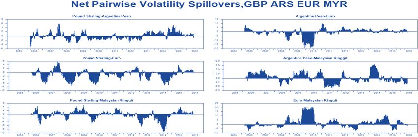
5.3. Return and Volatility Spillovers: Dynamic Analysis (Spillover Plots)
To address the extent of the spillover effect between developed and developing
countries we use 200-day rolling samples, which is about six months. The 200-day rolling
sample was used to demonstrate the spillover variations over time between developed and
developing countries since the data we used spans over the time period 2005–2016. The
dynamic movement of return and volatility spillovers is designed to capture the effect of the
potential recurring movement of spillovers by using returns and volatility indexes shown
in Tables 3 and 4. The indexes are the sums of all variance decompositions represented in
the form of “contribution to others”. Employing the indexes, we estimate the model to
scrutinise the evolution of global foreign exchange markets during the time period of the
sample (2005–2016). Hence, we capture the magnitude and disparities of the spillovers for
return and volatility, which we present graphically in the form of spillover plots.
The era of the 2000s, which began with a recession, mainly in developed countries
across the European Union and the USA undisputedly, documented painful economic
events in our history, in particular, the 2008 global financial turmoil. Thus, Figure 1 (return
spillovers) captures some of the critical events, whereas Figure 2 (volatility spillovers)
appears to be the most eventful. Interestingly, the 200-day rolling samples epitomised in
Figures 1 and 2 highlight some of the significant economic events that occurred during the
time period of the sample (2005–2016). As the estimation window moves towards 2016, we
captured the following critical economic events:
(1) The U.S. housing bubble worries, according to Liebowitz (2009) foreclosure rates,
increased by 43 per cent during the second and the fourth quarter of 2006.
(2) The increase in foreclosures and mortgage default rates reached about 55 per cent
(prime) and 80 per cent (subprime), which hugely devalued mortgage-back-securities
at the end of 2007, causing a severe credit crunch.
(3) In addition, in 2007, the British bank Northern Rock collapsed.
(4) Then, Lehman Brothers, the biggest U.S. investment bank, filed for bankruptcy on
15 September 2008.
(5) The above events, among others, were followed by the worst financial turmoil
(2007–2009) since the great depression (1929–1939), and the Greece debt crisis (De-
cember 2009).
(6) The European sovereign debt crisis occurred in 2009.
(7) The crude oil prices fell in 2014.
(8) The leading causes of the Russia financial crisis (2014–2017), according to the Centre
for Eastern Studies (OSW) were the tensions between Russia and the west, which led
to a sanction war and a dramatic fall in oil prices.
(9) First signs of Brexit worries began on 23 June 2016, whereby the British pound sterling
plunged to its lowest level since 1985.
The graphical illustrations in Figures 1 and 2 highlight important economic events
during the time period of the sample (2005–2016). The analysis orchestrated here, visually
signals the effect of volatility spillovers across intra-foreign exchange markets. The magni-
tude and extent of the spillover effect of both returns (Figure 1) and volatility (Figure 2)
were significantly marked by the crisis episodes of (2007–2009), in particular, the series
of European sovereign debt crisis (2009–2014) and the China stock market crash (2015),
among others. This means, interestingly, besides volatility spillovers, the contribution
of return spillovers is unexpectedly significant enough to show some commonality with
volatility spillovers in terms of responding to economic events.
Furthermore, we also observe bursts in total return and volatility spillovers which
materialise twice in Figure 1 and four times in Figure 2. The total return’s spillover began
to decrease slightly after its strong response to the (2007–2009) financial turmoil as well
as the European sovereign debt crisis in 2009 until the China stock market crash in (2015),
whereby it shows a dramatic increase.J. Risk Financial Manag. 2021, 14, x FOR PEER REVIEW 16 of 30
J. Risk Financial Manag. 2021, 14, 270 16 of 30
Figure 1.
Figure 1. Spillover
Spillover plot.
plot. Global foreign
foreign exchange
exchange market
market returns
returns (2005–2016).
(2005–2016).J. Risk Financial Manag. 2021, 14, 270 17 of 30
J. Risk Financial Manag. 2021, 14, x FOR PEER REVIEW 17 of 30
Figure 2. Spillover plot. Global foreign exchange market volatility (2005–2016).J. Risk Financial Manag. 2021, 14, 270 18 of 30
On the contrary, volatility spillovers fluctuate with explicit outbursts virtually with ev-
ery single economic event highlighted during the time period of the full sample (2005–2016).
In other words, the volatility spillover plot (Figure 2) depicts the phenomenon of the global
systemically important financial institutions from a series of historical defaults involved
that are too big to fail nature. To check the robustness of the results regarding rolling
window width, forecast horizon, and VAR ordering, we perform spillover plots (Figure 3)
using 84-day rolling window width, we also used two different variance decomposition
forecast horizons, i.e., a 70-day forecast horizon in Figure 3a and 14-day forecast horizon in
Figure 3b. The results are robust even when employing maximum and minimum volatility
spillovers across a diversity of alternative VAR ordering using 200-day rolling windows
(see Figures 3 and 4).
5.4. Robustness Analysis
According to the extent of the above results, the maximum and minimum spillovers
(Figure 4) show the variability of the volatility spillovers’ magnitude in global foreign ex-
change markets, which appears to be relatively higher than the return spillovers. Notwith-
standing, we find the behaviour of return spillovers in the global currency markets
(Figure 1) substantially responding to major economic events. Since we find “contribution
to others” mainly dominated by developed countries, in particular, the British pound
sterling (GBP), the Euro (EUR), and the Australian dollar (AUD), this means developing
countries act as net receivers to return and volatility spillovers.
Furthermore, according to the Bank for International Settlements’ (BIS) report (2013),
the USD, EUR, GBP, AUD, CAD, JPY, and CHF are the most traded currencies globally, and
account for almost 90 per cent of the global foreign exchange turnover. This means that a
substantial amount of return and volatility spillovers transmitted across the world during
the time period of the full sample (2005–2016) are coming from developed countries. The
findings are robust even when employing maximum and minimum volatility spillovers
across a diversity of alternative VAR ordering using 200-day rolling windows.
Interestingly, the results highlight the significance of the global foreign exchange
markets’ spillover channels during crisis periods in several dimensions. First, the results
highlight the cyclical bursts in spillovers that occur as a consequence of significant eco-
nomic events. These include the credit crunch of July 2007, Lehman Brothers collapsed in
September 2008, the financial turmoil which created havoc during 2007–2009, the European
sovereign debt crisis (2009–2014), and the fall in crude oil prices in 2013.
Secondly, the results highlight the potential magnitude of the spillover effect, in
particular, from the default of systemically important financial institutions across the global
financial system, which spread jitters from the outset of the U.S. subprime mortgage crisis.
Third, the results highlight the size of the shocks which led to bursts in spillovers (see
Figures 1–4) suggest strong cross-market interconnectedness. This reflects the definition
of contagion presented by Forbes and Rigobon (2002) as a significant increase in cross-
market linkages after a shock to one country or group of countries. Fourth, the results also
provide significant insights, particularly to the financial regulators, from the perspectives of
understanding the effect of spillovers from the default of systemically important financial
institutions. Finally, the results also introduce, for investors, the issue of cross-market
linkages and economic interdependence during crises periods, whereby volatility spillovers
increase substantially.J.J.Risk
RiskFinancial
FinancialManag.
Manag.2021,
2021,14,
14,270
x FOR PEER REVIEW 18 of 30 19 of 30
Figure3.3.Spillover
Figure Spilloverplots.
plots.Global
Globalforeign
foreignexchange
exchangemarkets
markets(2005–2016),
(2005–2016),70-
70-and
and14-day
14-dayforecast
forecasthorizons.
horizons.J. Risk Financial Manag. 2021, 14, 270 20 of 30
J. Risk Financial Manag. 2021, 14, x FOR PEER REVIEW 19 of 30
Figure
Figure4.
4.Maximum
Maximumand
andminimum
minimumspillovers.
spillovers.Global
Globalforeign
foreignexchange
exchangemarkets
markets(2005–2016).
(2005–2016).J. Risk Financial Manag. 2021, 14, 270 21 of 30
6. Time-Varying Volatility Spillovers
In this section, we present the results of the time-varying volatility spillovers among
developed and developing countries using autoregressive conditional heteroskedasticity
(ARCH). Time-varying volatility helps to investigate sources of significant shifts in the
volatility during the time period of our sample (2005–2016). This is because an ARCH
model is designed to capture persistence in time-varying volatility based on squared returns
Poon (2005). The ARCH model has a unique structure, where ”autoregressive” means high
volatility tends to persist, ”conditional” refers to time-varying or specific point on time,
and ”heteroskedasticity” refers to non-constant volatility Poon (2005). Before applying
the ARCH (1) model, we first generate the squared residuals using regression, which
contains only an intercept. Table 5 shows the regression result of the squared residuals.
This is because the squared residuals ensure that the conditional variance is positive and,
consequently, the leverage effects cannot be captured by the ARCH model Engle (2001).
Table 5. Regression results (squared residuals).
Variable Adjusted t* p-Value
Ehat2 8.12 0.000
No-of-Obs: 2.871 R-Squared: 0.022 Adj R-Squared: 0.002 MSE: 1.3 × 10⁻⁷
Second, we test the data for the presence of ARCH effects using the Box–Pierce large
multiplier (LM), which provides the most appropriate results Alexander (2002). Table 6
displays the result of the large multiplier’s (LM) test for the presence of ARCH effects in
the data.
Table 6. LM test results for autoregressive conditional heteroskedasticity (ARCH).
lags(p) chi2 df Prob > chi2
1 1 64.443 0.0000
H0, no ARCH effects vs. H1, ARCH (p) disturbance.
The LM results show the null and alternative hypotheses, the statistic and its distri-
bution, and the p-value, which indicates the presence of ARCH (p) model disturbance in
the data. Thus, we estimate the ARCH (1) model and generate the forecast error variance,
which is essentially an in-sample prediction model based on the estimated variance func-
tion (see Equation (19) for more details). Table 7 shows the result of the conditional variance
of the estimated ARCH (1) model. The conditional variance in the ARCH model is allowed
to change over time as a function of past error leaving the unconditional variance constant
Bollerslev (1986). Then, we proceed by plotting the forecast error variance against the time
period of our sample (2005–2016). Figure 5 shows the result of the ARCH (1) model, which
implies that the volatility spillovers from developed countries to the developing countries
seem to be specifically strong in 2008.
Table 7. ARCH (1) conditional variance for global foreign exchange market (2005–2016).
496 2.8 × 10⁻⁹ 2.8 × 10⁻⁹
497 2.24 × 10⁻⁹ 2.24 × 10⁻⁹
498 2.99 × 10⁻⁹ 2.99 × 10⁻⁹
499 2.56 × 10⁻⁹ 2.56 × 10⁻⁹
500 4.02 × 10⁻⁹ 4.02 × 10⁻⁹You can also read