Unconstrained Estimation of VLBI Global Observing System Station Coordinates
←
→
Page content transcription
If your browser does not render page correctly, please read the page content below
Adv. Geosci., 55, 23–31, 2021
https://doi.org/10.5194/adgeo-55-23-2021
© Author(s) 2021. This work is distributed under
the Creative Commons Attribution 4.0 License.

Unconstrained Estimation of VLBI Global Observing
System Station Coordinates
Markus Mikschi1 , Johannes Böhm1 , and Matthias Schartner1,2
1 Department     of Geodesy and Geoinformation, TU Wien, Wiedner Hauptstraße 8, 1040 Vienna, Austria
2 Institute   of Geodesy and Photogrammetry, ETH Zürich, Robert-Gnehm-Weg 15, 8093 Zürich, Switzerland

Correspondence: Markus Mikschi (markus.mikschi@geo.tuwien.ac.at)

Received: 29 June 2020 – Revised: 5 December 2020 – Accepted: 25 January 2021 – Published: 26 February 2021

Abstract. The International VLBI Service for Geodesy and          number of observations, thereby enabling an improved es-
Astrometry (IVS) is currently setting up a network of smaller     timation of tropospheric parameters which are considered
and thus faster radio telescopes observing at broader band-       one of the major error sources in geodetic VLBI (Schuh
widths for improved determination of geodetic parameters.         and Böhm, 2013). A recent demonstration of the possibili-
However, this new VLBI Global Observing System (VGOS)             ties with VGOS based on a single baseline between WEST-
network is not yet strongly linked to the legacy S/X network      FORD (USA) and the station GGAO12M (USA) is provided
and the International Terrestrial Reference Frame (ITRF) as       by Niell et al. (2018).
only station WESTFORD has ITRF2014 coordinates. In this              With the number of publicly available VGOS sessions ris-
work, we calculated VGOS station coordinates based on pub-        ing, accurate station coordinates for the participating sta-
licly available VGOS sessions until the end of 2019 while         tions become more important, e.g. for the estimation of Earth
defining the geodetic datum by fixing the Earth orientation       Orientation Parameters (EOP) in general or the estimation
parameters and the coordinates of the WESTFORD station in         of UT1-UTC from VGOS Intensive sessions in particular.
an unconstrained adjustment. This set of new coordinates al-      Furthermore, it is necessary to properly connect the VGOS
lows the determination of geodetic parameters from the anal-      network with the International Terrestrial Reference Frame
ysis of VGOS sessions, which would otherwise not be pos-          (ITRF). This enables the combination and comparison of
sible. As it is the concept of VGOS to use smaller, faster        VLBI analysis results from S/X and VGOS sessions which
slewing antennas in order to increase the number of obser-        is critical for the further development and testing of VGOS.
vations, shorter estimation intervals for the zenith wet delays   Thus, this work aims to provide accurate VGOS station co-
and the tropospheric gradients along with different relative      ordinates. The main challenge is caused by the fact that the
constraints were tested and the best performing parametriza-      datum has to be defined without accurate a priori coordinates
tion, judged by the baseline length repeatability, was used for   of most stations.
the estimation of the VGOS station coordinates.                      In Sects. 2, 3 and 4, we describe the existing VGOS data
                                                                  set, our methodology of calculating station coordinates, and
                                                                  the results, respectively. Additionally, we investigate the opti-
                                                                  mal parametrization of tropospheric parameters in Sect. 4.1,
1   Introduction                                                  which might be different for VGOS sessions compared to
                                                                  S/X sessions.
In order to improve the accuracies of geodetic parameters
determined with Very Long Baseline Interferometry (VLBI)          1.1   Definition of the Geodetic Datum
observations, the International VLBI Service for Geodesy
and Astrometry (IVS) (Nothnagel et al., 2017) has developed       Normally, at least three stations participating in a session
the VLBI Global Observing System (VGOS) (Petrachenko              need accurate a priori coordinates in the target terrestrial ref-
et al., 2009). This new system is based on smaller and faster     erence frame for the definition of the geodetic datum. These
VLBI radio telescopes, allowing for a significantly increased     stations should be globally well distributed and a higher

Published by Copernicus Publications on behalf of the European Geosciences Union.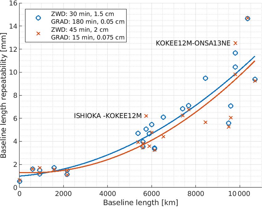
24                                                                            M. Mikschi et al.: VGOS Station Coordinates

number of stations is beneficial for making the datum defi-         – Free Adjustment. This is the most commonly used da-
nition redundant. Since so far, no VGOS observations have             tum definition method during the analysis of geodetic
been used in calculating a solution of the ITRF, it is dif-           VLBI sessions. In this method, also known as the mini-
ficult to proceed with standard approaches relying on No-             mal constraint method, carefully selected reference sta-
Net-Translation (NNT) and No-Net-Rotation (NNR) condi-                tions with very accurate a priori coordinates (x, y, z) are
tions on a priori ITRF coordinates of at least three stations.        selected as the datum stations. Their a priori coordinates
Among the VGOS telescopes, only WESTFORD is listed in                 are used together with the estimated additions to the a
the ITRF2014 (Altamimi et al., 2016) based on earlier S/X             priori coordinates (dx, dy, dz) to form the NNT/NNR
observations with this telescope. Between 2011 and 2014,              conditions. The NNT conditions stipulate that the sum
WESTFORD was converted to a VGOS station by a re-                     of the estimated additions to the a priori coordinates of
ceiver change (Niell et al., 2018). While the ITRF2014 co-            the datum stations along all three axes has to be zero.
ordinates of WESTFORD are derived from the S/X observa-               Similarly, the NNR conditions ensure that the sum of
tions, we can safely assume that the coordinates are the same         rotations about all three axes is zero.
for VGOS observations since the coordinates refer to the in-          The NNT and NNR conditions are represented as the
tersection point of the axes and are not related to the receiver      matrix-vector multiplication Gdx = 0. Subsequently
(Nothnagel, 2018).                                                    the N matrix is extended by G. The extended matrix
   The VLBI observations themselves define the relative po-           is now regular and the equation system can be solved.
sition of the stations w.r.t each other, the inner network ge-        Therefore, Eq. (1) becomes Eq. (2).
ometry, but not their absolute position and orientation with                            −1  T
                                                                                N GT

respect to a specific reference frame. This results in a singular       dx                   A Pl
                                                                            =                                           (2)
equation system during the least squares adjustment because              k      G 0            0
the design matrix and subsequently the normal equation ma-
                                                                      The benefit of this method is that the coordinates of the
trix have a rank deficiency corresponding to the degrees of
                                                                      datum defining stations are still estimated and their ac-
freedom (DOF) of the network. In the case of VLBI analysis,
                                                                      curacy can be calculated. Furthermore, the datum can be
the DOF is six, where three degrees are related to the rota-
                                                                      defined redundantly by selecting more datum stations
tion and the remaining three are related to the translation of
                                                                      than the minimum number of three, placing less empha-
the network. There is no scale ambiguity because the scale
                                                                      sis on any individual station and potential errors in its
is defined directly by the VLBI observations. The definition
                                                                      a priori coordinates. Because of this and the fact that
of the geodetic datum solves that rank deficiency, also called
                                                                      a good global distribution of the selected stations im-
a datum deficiency, and embeds the network geometry in a
                                                                      proves the datum definition, most of the time more than
reference frame.
                                                                      three stations are used in VLBI analysis.
   In the VLBI analysis the least squares approach is used
to estimate the most likely values of selected parameters x         – Unconstrained Adjustment. In this method the datum
based on a linearized over-determined equation system with            deficiency is alleviated by not estimating certain param-
observations affected by random errors. If the individual ob-         eters and therefore fixing them to their a priori values.
servations can be expressed solely as a function of the pa-           Just enough parameters are fixed such that the datum de-
rameters that are estimated, as is the case with VLBI obser-          ficiency is resolved but no constraints or distortions are
vations, the general case of the least squares approach can be        introduced to the inner network geometry. The param-
simplified using the Gauss-Markov model (Niemeier, 2008).             eters are fixed by removing the corresponding columns
Thereby, the corrections for the a priori parameters dx can           of the Jacobian matrix A or equivalently removing the
be estimated using                                                    corresponding columns and rows of the normal equa-
                                                                      tion matrix N. The benefit of this method is that fewer
dx = N−1 AT Pl                                               (1)      and potentially more precise a priori values can be used
                                                                      to define the geodetic datum with a potential improve-
with A being the Jacobian matrix containing the partial               ment in the estimated parameter accuracy. A drawback
derivatives of the functional model w.r.t the estimated param-        of this method is that the fixed parameters are not es-
eters and AT the transposed matrix, P denoting the weight             timated and their a priori values are considered as the
matrix for the observations and l the vector “observed” mi-           true values. Furthermore, the datum definition cannot
nus “computed with a priori values”. N is called the normal           be made redundant since fixing more parameters than
equation matrix and is computed using AT PA. In the pres-             necessary imposes a constraint on the inner network ge-
ence of a datum deficiency the matrix is singular and thus            ometry which would potentially contradict the obser-
Eq. (1) cannot be solved.                                             vations. An adjustment in which more parameters than
   There are two methods of defining the geodetic datum in            necessary are fixed to their a priori values is called an
a least squares adjustment for the VLBI analysis without af-          constrained adjustment. However, it has no relevance
fecting the inner network geometry:                                   for the task described here.

Adv. Geosci., 55, 23–31, 2021                                                      https://doi.org/10.5194/adgeo-55-23-2021
M. Mikschi et al.: VGOS Station Coordinates 25
1.2 Tropospheric delay parametrization by this. Since no velocities are estimated from the VGOS
data in our study, the CONT17 sessions should not act as
Tropospheric delays are generally modelled as the delay in leverage observations and therefore should not skew the esti-
zenith direction related to the delay at any given observa- mated parameters in a significant way. It was opted to include
tion elevation angle by a mapping function (Nilsson et al., the CONT17 sessions for an increase in observations.
2013). In this study, we use the Vienna Mapping Functions Figure 2 depicts the resulting station network. In general,
3 (Landskron and Böhm, 2018). The modelled delay is di- VLBI suffers from an imbalance of station distribution since
vided into a hydrostatic and a wet delay. While the hydro- there are far more stations in the northern than in the south-
static zenith delay can be determined from pressure measure- ern hemisphere (Plank et al., 2015). This imbalance is even
ments at the stations (see Saastamoinen, 1972 and Davis et more pronounced for the VGOS station network, as all sta-
al., 1985), the modelling of the wet delay is more difficult. tions available for this study are in the northern hemisphere
Thus, zenith wet delays (ZWD) are estimated in the VLBI with concentrations in Europe and the East Coast of the USA.
analysis. To account for azimuthal asymmetries in the tro- However, since the aim of this study was to estimate station
pospheric delays, so-called horizontal tropospheric gradients coordinates within an existing TRF and not to estimate a TRF
are also estimated. The ZWD and gradients are varying phe- there should not be strong effects of this imbalance. The fact
nomena and as such have to be parametrized in a way that that most stations are rather close to WESTFORD should in
allows for temporal variability while keeping the number fact benefit the accuracy of the estimated coordinates because
of estimated parameters low in order to maintain an over- of the used datum definition (see Sect. 3.1).
determined equation system. This can be achieved by using
piecewise linear offsets (PWLO) for the parametrization of
the ZWD and gradients (Schuh and Böhm, 2013). PWLO 3 Methodology
are based on offsets at certain reference epochs and linear
interpolation in between. Typically used estimation interval All analyses were carried out with the Vienna VLBI and
lengths are 30 min for the ZWD and 180 min for the gradi- Satellite Software (VieVs) (Böhm et al., 2018) following the
ents. Those values are used by the Vienna VLBI analysis cen- Conventions 2010 of the International Earth Rotation and
ter as of the time of writing. Additionally, relative constraints Reference Systems Service (IERS) (Petit and Luzum, 2010)
between the offsets can be introduced to increase numeri- and their updates.
cal stability and avoid singularity issues caused by too few
observations during any given estimation interval. The con- 3.1 Station coordinate estimation
straints are realized as pseudo-observations, stipulating that
the parameter at epoch ti+1 has to be equal to the parameter First, we ran single session analyses in order to detect and re-
at ti . The strength of the constraint is set by the associated move session anomalies, such as clock breaks. This prepara-
accuracy of the pseudo-observation during the least squares tory step is characterized by an iterative determination of ap-
adjustment. proximate station coordinates, which allows the detection of
problems within the sessions and the continuation with the
next steps.
2 Data Subsequently a first global solution was calculated by
solving all sessions together in a multi-year solution. The
For this study 30 VGOS sessions from 2017 and 2019 global solution uses a combination of the datum free normal
were used. Five sessions in 2017 were observed as part equation matrices of the single session analysis to estimate
of the CONT17 campaign (see https://ivscc.gsfc.nasa.gov/ parameters with higher accuracy (Schuh and Böhm, 2013).
program/cont17/, last access: 24 February 2021) and there- The geodetic datum for the global solution was defined in
fore are concentrated in December 2017. The remaining 25 an unconstrained adjustment by fixing some parameters to
are distributed over 2019. All sessions lasted for 24 h and their a priori values, as described in Sect. 1.1. There are mul-
the names of the sessions along with the participating sta- tiple possible combinations of fixed parameters that can al-
tions can be seen in Fig. 1. The CONT17 sessions started at leviate the datum deficiency. In this study, the coordinates of
23:00 UTC while the sessions in 2019 started at 18:00 UTC. the station WESTFORD were fixed to the ITRF2014 solution
Potential effects of the cluster of CONT17 sessions were and the EOP were fixed to the IERS14 C04 (Bizouard et al.,
investigated. The difference in the estimated coordinates, 2019) time series in an unconstrained adjustment. Since the
when the five CONT17 sessions are excluded, is below EOP describe the transformation between the terrestrial ref-
1.5 mm for all stations except for ISHIOKA and the z- erence frame (TRF) and the celestial reference frame (CRF),
coordinate of KOKEE12M. The larger differences for ISH- fixing them results in the TRF being tied to the CRF. There-
IOKA are to be expected since five of seven sessions in which fore, the three DOF describing the rotation of the TRF are
ISHIOKA participated are in 2017. As ISHIOKA is the clos- accounted for by the datum definition of the CRF. Fixing
est station to KOKEE12M, its coordinates are also influenced the coordinates of the station WESTFORD addresses the re-
https://doi.org/10.5194/adgeo-55-23-2021 Adv. Geosci., 55, 23–31, 202126 M. Mikschi et al.: VGOS Station Coordinates
Figure 1. Station activity during the VGOS sessions used in this study. The first five sessions were part of the CONT17 campaign. ISHIOKA
does only have VGOS observations during CONT17 and at the end of 2019. In between, it participated in S/X sessions.
Table 1. Sources of station velocities. The velocity for all but one
station was taken from corresponding S/X stations except for ISH-
IOKA, where the velocity was derived from R1 and R4 sessions.
station source
WETTZ13S ITRF2014 velocity of WETTZELL
KOKEE12M ITRF2014 velocity of KOKEE
WESTFORD ITRF2014 velocity of WESTFORD
GGAO12M ITRF2014 velocity of GGAO7108
RAEGYEB ITRF2014 velocity of YEBES
ONSA13NE ITRF2014 velocity of ONSALA60
ONSA13SW ITRF2014 velocity of ONSALA60
ISHIOKA from global solution of R1 & R4 sessions
what would be achievable from the short VGOS time span.
However, one exception refers to station ISHIOKA (Japan)
as ISHIOKA’s velocities could not be fixed to the closest
ITRF2014 defining station, TSUKUB32. During tests with
velocity estimation in the global solution, the estimated ve-
locity of ISHIOKA was vastly different from the one listed
Figure 2. The VGOS station network used in this study. All stations
are located in the northern hemisphere. Onsala (Sweden) runs a twin in the ITRF2014 for TSUKUB32. To overcome this discrep-
VGOS telescope with a north-east (ONSA13NE) and a south-west ancy, the velocity of ISHIOKA was calculated using an in-
(ONSA13SW) dish. dependent global solution of 305 R1 and R4 (S/X) sessions
from 2017–2019 most of which ISHIOKA participated in.
The inconsistencies between the TSUKUB32 and the ISH-
maining three DOF of the translation of the network. Station IOKA station velocity might be explained by the strong tec-
WESTFORD was selected for this purpose since it is the only tonic activity in Japan. Table 1 summarizes the sources for
VGOS station with ITRF2014 coordinates. The positions of the station velocities.
the radio sources were fixed to their coordinates in ICRF3
(Charlot et al., 2020). 3.2 Troposphere parametrization test
Due to the limited time span of the VGOS data, the sta-
tion velocities were not estimated during the global solution, In order to investigate the effects of different troposphere
but instead fixed to velocities from co-located ITRF2014 S/X parametrizations on the VGOS sessions, the single session
stations. It was assumed that the velocities of the nearby S/X analysis was performed repeatedly, using a grid-wise com-
stations are identical with the velocities of the VGOS sta- bination of various ZWD and gradient estimation intervals
tions. This is a reasonable approach since the S/X station as well as different constraint accuracies for both parame-
velocities are known with a higher accuracy compared to ters. This leads to a four-dimensional parameter space that is
Adv. Geosci., 55, 23–31, 2021 https://doi.org/10.5194/adgeo-55-23-2021M. Mikschi et al.: VGOS Station Coordinates 27
Table 2. Tested values of the parametrization of the tropospheric
estimates.
Parameter Tested values
ZWD interval [min] 20, 30, 45, 60, 80
ZWD constraint accuracy [cm] 1, 1.5, 2
gradient interval [min] 15, 30, 60, 100, 180
gradient constraint accuracy [cm] 0.025, 0.05, 0.075
Table 3. Parametrization of the tropospheric estimates for the refer-
ence solution.
Parameter Estimation constraint [cm]
interval [min]
ZWD 30 1.50
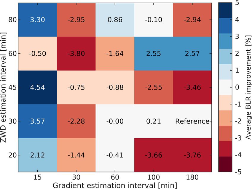
gradients 180 0.05 Figure 3. The average relative BLR change for a two-dimensional
slice from the four-dimensional parameter space along the interval
axes for constraints with 1.5 and 0.05 cm for the ZWD and gradi-
investigated. Similarly to the global solution, the datum defi- ents respectively. Blue color denotes improvement, red color degra-
nition of this single session analysis for the troposhpere anal- dation.
ysis was performed by fixing the EOP and the WESTFORD
station coordinates. Therefore, three sessions had to be ex-
4.1 Troposphere parametrization
cluded since WESTFORD did not participate (see Fig. 1).
The tested values for the different parameters are listed in Ta- Table 4 lists the ten best performing parametrizations out of
ble 2. In total, these values lead to 225 different parametriza- the 225 tested setups, along with the resulting average BLR
tions. improvement. As can be seen, best results can be achieved by
The performance of individual parametrizations was as- using shorter estimation intervals for the gradients combined
sessed based on the average relative improvement of the with slightly longer estimation intervals for the ZWD com-
baseline length repeatability (BLR) compared to a reference pared to the reference parametrization that is typically used
solution. For a specific parametrization the BLR of all base- for S/X observations. The six best parameter sets all utilize
lines was calculated and then individually compared to the the combination of 15 and 45 min estimation intervals for the
corresponding BLR from the reference solution. The relative gradients and the ZWD, respectively, with various combina-
improvement of all BLRs for one parametrization was aver- tions of the associated constraints.
aged to obtain the final metric. The reference solution was Figure 3 depicts a two-dimensional slice from the four-
derived by selecting a tropospheric parametrization that is dimensional parameter space along the interval axes. Since
typically used for analyzing S/X observations (see Table 3). the constraints do not affect the solution that much, this en-
By investigating the relative improvement of the BLR com- ables to easier compare the improvement based on the dif-
pared to a reference solution instead of a mean BLR, the de- ferent intervals. The importance of short gradient estimation
pendency on the baseline length can be taken into account, intervals is emphasized as a 15 min interval yields the best
as longer baselines tend to have a worse BLR. results. One exception refers to a ZWD interval of 60 min
After the best performing troposphere parametrization where longer gradient intervals lead to a better result. The
had been found, the global solution was calculated again reason for this behaviour is unknown and subject to further
as described previously using the improved troposphere investigation.
parametrization to estimate the final station coordinates with The selection of the ZWD constraints appears to have a
highest precision. smaller impact on the result. This could be somehow ex-
pected since all three constraint values are rather loose and
4 Results only help to stabilize the solution in case of missing observa-
tions between estimation epochs. As far as the gradient con-
In this section we first investigate the optimal tropospheric straints are concerned, the highest value (loosest constraint)
parametrization for the VGOS sessions. Then, we present is yielding the best BLR. This again confirms the impor-
the VGOS station coordinate estimates resulting from the tance of rapid and flexible gradient estimates with VGOS, as
unconstrained adjustment utilizing the best tropospheric tighter constraints would eliminate some of the freedom in
parametrization as described in Sect. 3. the estimation gained by the short estimation intervals. How-
ever, also for the tightest tested constraints, the combination
https://doi.org/10.5194/adgeo-55-23-2021 Adv. Geosci., 55, 23–31, 202128 M. Mikschi et al.: VGOS Station Coordinates
Table 4. The ten best performing troposphere parametrizations out of the 225 tested parametrizations along with the resulting average BLR
improvement.
Average BLR ZWD ZWD Gradient Gradient
improvement [%] interval [min] constraint [cm] interval [min] constraint [cm]
4.88 (best) 45 1.5 15 0.075
4.88 45 1 15 0.07
4.86 45 2 15 0.075
4.54 45 1.5 15 0.05
4.53 45 2 15 0.05
4.47 45 1 15 0.05
3.60 30 1 15 0.05
3.57 30 1.5 15 0.05
3.54 30 2 15 0.05
3.52 80 2 15 0.075
of 15 and 45 min estimation intervals for the gradients and
ZWD, respectively, yields the best results.
The average BLR improvement suggests that shorter in-
tervals do in fact benefit the modeling of real troposphere
variations and not just absorb measurement noise. Further-
more, significant changes in the tropospheric delays at low
elevations may occur more often, making the rapid gradient
estimation more beneficial than the rapid estimation of ZWD.
This also holds true for S/X observations and an optimization
of the parametrization of these sessions might also be war-
ranted. However, the lower number of observations and the
reduced sky-coverage of S/X observations make rapid tro-
posphere parameter estimation difficult. The smaller, faster
slewing VGOS antennas enable more observations and a bet-
ter sky-coverage. Figure 4 shows the number of observations
per hour for the different VGOS stations along with the data
for all stations of the R1 and R4 sessions during 2019 for Figure 4. Number of observations per hour for the VGOS stations
as boxplots. Boxplot for all stations for the R1 and R4 sessions of
comparison. The plot is based on the scheduling files (.skd)
2019 added for comparison.
of the sessions.
The DOF of a least squares adjustment utilizing such a
parametrization is of course lower when compared to the ref-
erence parametrization. However, the used VGOS sessions two notable exceptions being ISHIOKA–KOKEE12M and
of 2019 still have an average DoF of 5411 or an average ratio KOKEE12M–ONSA13NE. The degradation of the BLR for
between observations and parameters of about 4.8. Therefore those two baselines can be explained by the lower number
we think it is worth the trade-off. Additionally, the introduced of observations per time for the station KOKEE12M, as can
relative constraints minimize adverse effects of the shorter be seen in Fig. 4. The reason for the lower number of ob-
estimation interval. servations is the network geometry as KOKEE12M is quite
Although sophisticated simulations (Petrachenko et al., secluded from the rest of the network (see Fig. 2). This prob-
2009) already indicated that rapid gradients will be benefi- lem is expected to be solved by the growth of the VGOS net-
cial for VGOS analysis, this is the first time to see this ef- work, as well as improved SNR based scheduling approaches
fect with real data. It is expected that the improvement will which should yield more observations overall.
even be more visible with further optimized VGOS schedules Consequently, this parametrization defined in the first row
(Schartner and Böhm, 2020). of Table 4 is used for the determination of the VGOS station
The BLR with the reference parametrization that is usu- coordinates. The difference of the estimated station coordi-
ally used in the analysis of S/X observations (Table 3) along nates in the global solution between the best and the refer-
with the BLR with the best parametrization found within ence parametrization is depicted in Fig. 6 in the local east,
this study is visualized in Fig. 5. It is evident that im- north, and up components. The European stations exhibit
provements were achieved for almost all baselines with the similar shifts while the difference of coordinate estimates for
Adv. Geosci., 55, 23–31, 2021 https://doi.org/10.5194/adgeo-55-23-2021M. Mikschi et al.: VGOS Station Coordinates 29
ities were estimated from R1 and R4 S/X sessions in the time
span 2017 to 2019.
The formal errors were obtained from the unconstrained
least squares adjustment of the global solution. Therefore,
they only capture the accuracy of the inner network geom-
etry. In the chosen datum definition method, the EOP and
WESTFORD coordinates are seen as true values and not as
stochastic quantities during the adjustment. Inaccuracies in
those values directly affect the estimated station coordinates
but do not show up in the estimated formal errors. Addition-
ally, errors in the a priori models pertaining to the station
coordinates of WESTFORD also directly influence the es-
timation results. Therefore, the listed formal errors are too
optimistic and not truly representative of the accuracies of
the absolute positions of the estimated stations. More realis-
tically, the absolute positional accuracy is at the few millime-
ter level.
Figure 5. Baseline length repeatability of the reference parametriza-
This is confirmed by a comparison with ISHIOKA coordi-
tion (blue) and the best parametrization (red) with a fitted second
degree polynomial approximation. nates. While ISHIOKA is not listed in ITRF2014, the analy-
sis of the S/X sessions also yielded coordinates that could be
used for comparisons with VGOS data. The total length of
the difference vector between the ISHIOKA positions from
the two different solutions is close to 1 cm. However, ISH-
IOKA’s accuracy might be comparatively worse, due to the
limited number of sessions it participated in (see Fig. 1) and
the fact that the long distance to WESTFORD accentuates
the error caused by noise or possible biases in the EOP data.
5 Conclusions
In this study we demonstrated how an unconstrained adjust-
ment can be used for the definition of the geodetic datum of
VLBI sessions to connect the VGOS network with the ITRF.
Therefore, the station coordinates of WESTFORD and the
five EOP were fixed to their a priori values. This approach
Figure 6. Difference in station coordinate estimates from a was later used during a global solution of 30 VGOS sessions
global solution between the best and the reference troposphere from 2017 and 2019 to estimate precise VGOS station coor-
parametrization in the local east, north, and up components. dinates.
In the future, it is assumed that the connection of the
VGOS network to the ITRF will also be done based on lo-
GGAO12M is very small, presumably due to the close prox- cal tie measurements and using local interferometer sessions.
imity to WESTFORD, which was fixed to its a priori val- However, up to this point none of these results are publicly
ues. ISHIOKA and KOKEE12M also exhibit larger changes available. Additionally, within the IVS, three special sessions
in the north component. This can be explained by the sky- RD2005–RD2007 are planned where VGOS stations observe
coverage at those stations, as the observations are limited to together with S/X stations in a mixed-mode. Results of these
one side of the sky due to the network configuration. sessions will be most valuable to connect the VGOS network
to the legacy S/X network. In 2021, several VGOS stations
4.2 VGOS station coordinates will be listed in ITRF2020, because the VGOS observations
will be used for the generation of the next ITRF. After this
The VGOS station coordinates as determined with the best point, the definition of the geodetic datum for VGOS ses-
parametrization of the troposphere in a global solution are sions can be done using NNR and NNT conditions again.
listed in Table 5 along with the formal errors σ . The veloci- In the course of this study, we also tested various
ties were not estimated but stem from co-located S/X stations parametrizations for the estimation of the tropospheric pa-
as described in Sect. 3.1. In the case of ISHIOKA, the veloc- rameters in terms of baseline length repeatability values, be-
https://doi.org/10.5194/adgeo-55-23-2021 Adv. Geosci., 55, 23–31, 202130 M. Mikschi et al.: VGOS Station Coordinates
Table 5. The VGOS station coordinates resulting from the final global solution using the best parametrization for the tropospheric parameters
and their formal uncertainties σ . The velocities v are taken from the ITRF2014 for co-located telescopes or were determined from X/S
sessions in the case of ISHIOKA.
Station x [m] y [m] z [mm] vx [mm/y] vy [mm/y] vz [mm/y] Epoch
σx [mm] σy [mm] σz [mm]
GGAO12M 1130729.8901 −4831245.9513 3994228.2858 −15.0 −1.1 2.3 2019.0
0.13 0.30 0.30 – – –
ISHIOKA −3959636.1631 3296825.4794 3747042.5982 −21.6 −4.1 −7.2 2019.0
0.79 0.63 1.03 – – –
KOKEE12M −5543831.7452 −2054585.6766 2387828.9132 −9.3 62.9 32.3 2019.0
0.76 0.57 0.65 – – –
ONSA13NE 3370889.1679 711571.3337 5349692.1367 −14.4 14.5 10.4 2019.0
0.29 0.28 0.51 – – –
ONSA13SW 3370946.6476 711534.6414 5349661.0136 −14.4 14.5 10.4 2019.0
0.32 0.29 0.57 – – –
RAEGYEB 4848831.0431 −261629.4098 4122976.5478 −4.9 19.0 16.5 2019.0
0.44 0.30 0.53 – – –
WETTZ13S 4075658.8769 931824.8827 4801516.2891 −16.1 17.0 10.0 2019.0
0.30 0.27 0.48 – – –
WESTFORD 1492206.3859 −4458130.5272 4296015.5872 −15.6 −1.3 4.1 2010.0
– – – – – –
cause VGOS observations are expected to better resolve the Special issue statement. This article is part of the special issue “Eu-
troposphere at the stations. This investigation revealed that ropean Geosciences Union General Assembly 2020, EGU Geodesy
shorter estimation intervals for the gradients of 15 min and Division”. It is a result of the EGU General Assembly 2020, 4–8
slightly longer estimation intervals of 45 min for the ZWD, May 2020.
compared to typical S/X analysis values, are beneficial. How-
ever, the ongoing maturing of VGOS, especially in terms of
improvements in its scheduling (Schartner and Böhm, 2020), Acknowledgements. The authors are grateful to the Austrian Sci-
ence Fund (FWF) for supporting this work with project VGOS
will likely continue to change the ideal parametrization of the
Squared (P 31625-N29).
tropospheric estimates.
We would like to thank all parties that contributed to the suc-
cess of the CONT17 campaign, in particular to the IVS Coor-
dinating Center at NASA Goddard Space Flight Center (GSFC)
Data availability. The used VGOS data is publicly available for taking the bulk of the organizational load, to the GSFC VLBI
from the Crustal Dynamics Data Information System (CDDIS group for preparing the legacy S/X observing schedules and MIT
DAAC; available at: https://cddis.nasa.gov/archive/vlbi/ivsdata/ Haystack Observatory for the VGOS observing schedules, to the
vgosdb/) (International VLBI Service for Geodesy and Astrometry, IVS observing stations at Badary and Zelenchukskaya (both In-
2021). stitute for Applied Astronomy, IAA, St. Petersburg, Russia), For-
taleza (Rádio Observatório Espacial do Nordeste, ROEN; Cen-
ter of Radio Astronomy and Astrophysics, Engineering School,
Author contributions. MM analysed the VGOS sessions, imple- Mackenzie Presbyterian University, Sao Paulo and Brazilian Insti-
mented a unconstrained adjustment for global solutions in VieVS tuto Nacional de Pesquisas Espaciais, INPE, Brazil), GGAO (MIT
and tested different troposphere parametrizations. JB helped with Haystack Observatory and NASA GSFC, USA), Hartebeesthoek
the tropospheric parametrization while MS provided guidance for (Hartebeesthoek Radio Astronomy Observatory, National Research
the unconstrained global solution. MM wrote the manuscript with Foundation, South Africa), the AuScope stations of Hobart, Kather-
input from JB and MS. ine, and Yarragadee (Geoscience Australia, University of Tasma-
nia), Ishioka (Geospatial Information Authority of Japan), Kashima
(National Institute of Information and Communications Technol-
Competing interests. The authors declare that they have no conflict ogy, Japan), Kokee Park (U.S. Naval Observatory and NASA
of interest. GSFC, USA), Matera (Agencia Spatiale Italiana, Italy), Medicina
(Istituto di Radioastronomia, Italy), Ny Ålesund (Kartverket, Nor-
Adv. Geosci., 55, 23–31, 2021 https://doi.org/10.5194/adgeo-55-23-2021M. Mikschi et al.: VGOS Station Coordinates 31
way), Onsala (Onsala Space Observatory, Chalmers University of International VLBI Service for Geodesy and Astrometry: VGOSDB
Technology, Sweden), Seshan (Shanghai Astronomical Observa- observation data, available at: https://cddis.nasa.gov/archive/
tory, China), Warkworth (Auckland University of Technology, New vlbi/ivsdata/vgosdb/ (last access: 24 February 2021), NASA
Zealand), Westford (MIT Haystack Observatory), Wettzell (Bun- EOSDIS CDDIS DAAC, Greenbelt, MD, USA, 2021.
desamt für Kartographie und Geodäsie and Technische Universität Landskron, D. and Böhm, J.: VMF3/GPT3: refined discrete and em-
München, Germany), and Yebes (Instituto Geográfico Nacional, pirical troposphere mapping functions, J. Geodesy, 92, 349–360,
Spain) plus the Very Long Baseline Array (VLBA) stations of the https://doi.org/10.1007/s00190-017-1066-2, 2018.
Long Baseline Observatory (LBO) for carrying out the observations Niell, A., Barrett, J., Burns, A., Cappallo, R., Corey, B., Derome,
under the US Naval Observatory’s time allocation, to the staff at the M., Eckert, C., Elosegui, P., McWhirter, R., Poirier, M., Ra-
MPIfR/BKG correlator center, the VLBA correlator at Socorro, and jagopalan, G., Rogers, A., Ruszczyk, C., SooHoo, J., Titus, M.,
the MIT Haystack Observatory correlator for performing the corre- Whitney, A., Behrend, D., Bolotin, S., Gipson, J., Gordon, D.,
lations and the fringe fitting of the data, and to the IVS Data Centers Himwich, E., and Petrachenko, B.: Demonstration of a broad-
at BKG (Leipzig, Germany), Observatoire de Paris (France), and band very long baseline interferometer system: A new instrument
NASA CDDIS (Greenbelt, MD, USA) for the central data holds. for high-precision space geodesy, Radio Sci., 53, 1269–1291,
https://doi.org/10.1029/2018RS006617, 2018.
Niemeier, W.: Ausgleichungsrechnung: Statistische Auswertemeth-
Financial support. This research has been supported by the Aus- oden, 2., De Gruyter, Berlin, Germany, 2008.
trian Science Fund (FWF) (grant no. P 31625-N29). Nilsson, T., Böhm, J., Wijaya, D. D., Tresch, A., Nafisi, V., and
Schuh, H.: Path Delays in the Neutral Atmosphere, in: Atmo-
spheric Effects in Space Geodesy, edited by: Böhm, J. and Schuh,
Review statement. This paper was edited by Mathis Bloßfeld and H., Springer, Berlin, Heidelberg, 73–136, 2013.
reviewed by two anonymous referees. Nothnagel, A., Artz, T., Behrend, D., and Malkin, Z.: International
VLBI Service for Geodesy and Astrometry, J. Geodesy, 91, 711–
721, https://doi.org/10.1007/s00190-016-0950-5, 2017.
Nothnagel A.: Very Long Baseline Interferometry, in: Handbuch der
References Geodäsie, edited by: Freeden W. and Rummel R., Springer Ref-
erence Naturwissenschaften, Springer Spektrum, Berlin, Heidel-
Altamimi, Z., Rebischung, P., Métivier, L., and Collilieux, berg, https://doi.org/10.1007/978-3-662-46900-2_110-1, 2018.
X.: ITRF2014: A new release of the International Ter- Petit, G. and Luzum, B.: IERS Conventions 2010, IERS Tech-
restrial Reference Frame modeling nonlinear station nical Note, 36, Verlag des Bundesamtes für Kartographie und
motions, J. Geophys. Res.-Sol. Ea., 121, 6109–6131, Geodäsie, Frankfurt am Main, 2010.
https://doi.org/10.1002/2016JB013098, 2016. Petrachenko, B., Niell, A., Behrend, D., Corey, B., Böhm, J.,
Bizouard, C., Lambert, S., Gattano, C., Becker, O., and Richard, Charlot, P., Collioud, A., Gipson, J., Haas, R., Hobiger, T.,
J. Y.: The IERS EOP 14C04 solution for Earth orientation pa- Koyama, Y., Macmillan, D., Malkin, Z., Nilsson, T., Pany, A.,
rameters consistent with ITRF 2014, J. Geodesy, 93, 621–633, Tuccari, G., Whitney, A., and Wresnik, J.: Design Aspects of
https://doi.org/10.1007/s00190-018-1186-3, 2019. the VLBI2010 System, Progress Report of the IVS VLBI2010
Böhm, J., Böhm, S., Boisits, J., Girdiuk, A., Gruber, J., Heller- Committee, Goddard Space Flight Center, Greenbelt, Mary-
schmied, A., Krásná, H., Landskron, D., Madzak, M., Mayer, land, available at: https://ivscc.gsfc.nasa.gov/publications/misc/
D., McCallum, J., McCallum, L., Schartner, M., and Teke, K.: TM-2009-214180.pdf (last access: 24 February 2021), 2009.
Vienna VLBI and Satellite Software (VieVS) for Geodesy and Plank, L., Lovell, J. E. J., Shabala, S. S., Böhm, J.,
Astrometry, PASP, 130, 044503, https://doi.org/10.1088/1538- and Titov, O.: Challenges for geodetic VLBI in the
3873/aaa22b, 2018. southern hemisphere, Adv. Space Res., 56, 304–313,
Charlot, P., Jacobs, C. S., Gordon, D., Lambert, S., de Witt, A., https://doi.org/10.1016/j.asr.2015.04.022, 2015.
Böhm, J., Fey, A. L., Heinkelmann, R., Skurikhina, E., Titov, O., Saastamoinen, J.: Atmospheric Correction for the Troposphere and
Arias, E. F., Bolotin, S., Bourda, G., Ma, C., Malkin, Z., Noth- Stratosphere in Radio Ranging Satellites, in: The Use of Artifi-
nagel, A., Mayer, D., MacMillan, D. S., Nilsson, T., and Gaume, cial Satellites for Geodesy, edited by Henriksen, S. W., Mancini,
R.: The Third Realization of the International Celestial Refer- A., and Chovitz, B. H., 15, 247–251, AGU, Washington, D.C.,
ence Frame by Very Long Baseline Interferometry, Astron. As- 1972.
trophys., submitted, 2020. Schartner, M. and Böhm, J.: Optimizing schedules for
Davis, J. L., Herring, T. A., Shapiro, I. I., Rogers, A. E. E., and the VLBI global observing system, J. Geodesy, 94, 12,
Elgered, G.: Geodesy by radio interferometry: Effects of atmo- https://doi.org/10.1007/s00190-019-01340-z, 2020.
spheric modeling errors on estimates of baseline length, Radio Schuh, H. and Böhm, J.: VLBI for Geodesy and Astrometry, in:
Sci., 20, 1593–1607, https://doi.org/10.1029/RS020i006p01593, Sciences of Geodesy II, Innovations and Future Developments,
1985. edited by: Xu, G., Springer, Berlin, 2013.
https://doi.org/10.5194/adgeo-55-23-2021 Adv. Geosci., 55, 23–31, 2021You can also read