Three-dimensional multiple-relaxation-time discrete Boltzmann model of compressible reactive flows with nonequilibrium effects
←
→
Page content transcription
If your browser does not render page correctly, please read the page content below

Three-dimensional multiple-relaxation-time
discrete Boltzmann model of compressible
reactive flows with nonequilibrium effects
Cite as: AIP Advances 11, 045217 (2021); https://doi.org/10.1063/5.0047480
Submitted: 20 March 2021 . Accepted: 01 April 2021 . Published Online: 18 April 2021

  Yu Ji (吉雨),       Chuandong Lin (林传栋), and        Kai H. Luo (罗开红)

ARTICLES YOU MAY BE INTERESTED IN

Double-D2Q9 lattice Boltzmann models with extended equilibrium for two-dimensional
magnetohydrodynamic flows
Physics of Fluids 33, 035143 (2021); https://doi.org/10.1063/5.0043998

A multiple-relaxation-time collision model for nonequilibrium flows
Physics of Fluids 33, 037134 (2021); https://doi.org/10.1063/5.0046866

Extended lattice Boltzmann model for gas dynamics
Physics of Fluids 33, 046104 (2021); https://doi.org/10.1063/5.0048029

AIP Advances 11, 045217 (2021); https://doi.org/10.1063/5.0047480                      11, 045217

© 2021 Author(s).
AIP Advances                                                                                   ARTICLE           scitation.org/journal/adv

    Three-dimensional multiple-relaxation-time
    discrete Boltzmann model of compressible
    reactive flows with nonequilibrium effects
    Cite as: AIP Advances 11, 045217 (2021); doi: 10.1063/5.0047480
    Submitted: 20 March 2021 • Accepted: 1 April 2021 •
    Published Online: 19 April 2021

    Yu Ji (吉雨),1           Chuandong Lin (林传栋),2,a)            and Kai H. Luo (罗开红)3,b)

    AFFILIATIONS
    1
      Center for Combustion Energy, Key Laboratory for Thermal Science and Power Engineering of Ministry of Education,
      Department of Energy and Power Engineering, Tsinghua University, Beijing 100084, China
    2
      Sino-French Institute of Nuclear Engineering and Technology, Sun Yat-sen University, Zhuhai 519082, China
    3
      Department of Mechanical Engineering, University College London, Torrington Place, London WC1E 7JE, United Kingdom

    a)
         Electronic mail: linchd3@mail.sysu.edu.cn
    b)
         Author to whom correspondence should be addressed: K.Luo@ucl.ac.uk

    ABSTRACT
    Based on the kinetic theory, a three-dimensional multiple-relaxation-time discrete Boltzmann model (DBM) is proposed for nonequilibrium
    compressible reactive flows where both the Prandtl number and specific heat ratio are freely adjustable. There are 30 kinetic moments of the
    discrete distribution functions, and an efficient three-dimensional thirty-velocity model is utilized. Through the Chapman–Enskog analysis,
    the reactive Navier–Stokes equations can be recovered from the DBM. Unlike existing lattice Boltzmann models for reactive flows, the hydro-
    dynamic and thermodynamic fields are fully coupled in the DBM to simulate combustion in subsonic, supersonic, and potentially hypersonic
    flows. In addition, both hydrodynamic and thermodynamic nonequilibrium effects can be obtained and quantified handily in the evolution
    of the discrete Boltzmann equation. Several well-known benchmarks are adopted to validate the model, including chemical reactions in the
    free falling process, thermal Couette flow, one-dimensional steady or unsteady detonation, and a three-dimensional spherical explosion in an
    enclosed cube. It is shown that the proposed DBM has the capability to simulate both subsonic and supersonic fluid flows with or without
    chemical reactions.
    © 2021 Author(s). All article content, except where otherwise noted, is licensed under a Creative Commons Attribution (CC BY) license
    (http://creativecommons.org/licenses/by/4.0/). https://doi.org/10.1063/5.0047480

    I. INTRODUCTION                                                          nonequilibrium effects as well as the complex interplay between the
                                                                             chemical reaction and fluid flow. Moreover, these processes cover a
         Reactive flows encompassing a wide variety of nonlinear,            wide range of spatial and temporal scales.3–6 In order to study the
    unsteady, and nonequilibrium processes are common in nature and          reactive flow in detail, experimental techniques have been widely
    industry.1 In fact, more than four-fifths of mankind’s utilized energy   used.7,8 However, experiments for supersonic and hypersonic reac-
    is generated from the exothermic reactive flows.2 In the past few        tive flows are difficult and expensive to conduct; and the measure-
    decades, considerable research has been devoted to reactive flows,       ments are usually global quantities only. On the other hand, numer-
    including supersonic and hypersonic flows related to the super-          ical simulations provide a convenient tool for relevant research and
    sonic aircraft, rocket engine, detonation engine, supersonic com-        become more and more reliable and cost-effective.
    bustion ramjet, etc. However, there are still many problems that               The supersonic reactive flow modeling approaches can gen-
    have not been solved due to the complex physical and chemical            erally be classified into three groups. The first group is the con-
    processes involved, such as high compressibility, strong flow dis-       ventional simulation methods based on the continuum assump-
    continuity, and combustion instability. In addition, these processes     tion, such as direct numerical simulation,9 large eddy simulation,10
    are usually accompanied by the hydrodynamic and thermodynamic            and Reynolds-averaged Navier–Stokes (NS).11 These conventional

AIP Advances 11, 045217 (2021); doi: 10.1063/5.0047480                                                                                  11, 045217-1
© Author(s) 2021
AIP Advances ARTICLE scitation.org/journal/adv
methods are good at capturing the main hydrodynamic character- be compressible, thermal, and, at the same time, coupling the
istics. However, they lack the ability to describe thermodynamic chemical reaction naturally. In addition, the model should take
nonequilibrium effects under highly nonequilibrated conditions, hydrodynamic and thermodynamic nonequilibrium effects into
such as the shock or detonation front.12,13 The second group is consideration.
the microscopic methods, like molecular dynamics.14 The molecu- In recent years, the discrete Boltzmann method (DBM) has
lar dynamics gets rid of the local equilibrium assumption and thus been constructed to model and simulate nonequilibrium systems,
can be used to study the detailed hydrodynamic and thermody- with various velocity and time–space discretization schemes.31–35,39
namic properties.15–17 On the other hand, the computational cost The DBM and LBM can be viewed as two distinctive classes of dis-
of molecular dynamics is usually prohibitive and the computational crete numerical methods based on the Boltzmann equation. Despite
domain is always limited. The third group is the kinetic method14 sharing the same origin and some similarities, the objectives, numer-
based on the Boltzmann equation, which removes the limit of the ical implementation, and capabilities of the LBM and DBM are dif-
local equilibrium assumption. A kinetic method, the lattice Boltz- ferent. Basically, the LBM aims to recover the macroscopic behav-
mann method (LBM), simulates the evolution of probability distri- iors of the flow system and acts as an alternative method to the
bution functions in a discretized phase-space, which can be related continuum-based Navier–Stokes solver. On the other hand, the
to macroscopic quantities by moment relationships. The LBM has DBM is a discrete Boltzmann equation solver that aims to keep
been successfully applied to simulate a variety of complex flows,18 some kinetic features that go beyond the macroscopic behaviors.
including reactive flows.19–36 Merits of the LBM include the algo- Numerically, discretization in space, time, and particle velocities
rithm simplicity and locality, which lead to excellent performance is inter-dependent in the LBM algorithm. In the DBM, however,
on parallel clusters. discretization in space, time, and particle velocities is decoupled,
The key to dealing with reactive flows in the LBM is how which allows a variety of numerical methods to be applied. As a
to describe the energy and species mass fractions by LB formula- result, the LBM requires different models for different types of flows
tion and couple them consistently. Current LBM formulations for (e.g., incompressible, compressible, thermal, or reactive), while a
reactive flows can be divided into two categories. The first cate- uniformed DBM framework can simulate all types of flows. More-
gory is the hybrid method, in which the flow simulation is accom- over, the DBM can capture both hydrodynamic and thermodynamic
plished through the weakly compressible LBM solver, while the nonequilibrium effects explicitly.
transport equations for energy and species are solved by a finite To some extent, the mathematical framework of the DBM is
difference scheme. In 2000, Filippova and Häenel proposed an similar to the rational extended thermodynamics (RET), which is
LBM for reacting flows at a low Mach number with variable den- also capable of explaining nonequilibrium phenomena. The RET
sity.20,21 Later, Hosseini et al. modified the LBM solver and success- proposed by Ruggeri and Sugiyama40,41 is motivated by the Boltz-
fully simulated premixed and non-premixed flames with a detailed mann equation. Different from the kinetic theory, the RET focuses
thermo-chemical model.22,23 In 2020, Shu et al. developed a sim- on the relations of the moments and forms a hierarchy of the bal-
plified sphere function-based gas-kinetic flux solver for compress- ance laws. To achieve the closure of the moments, the RET truncates
ible viscous reacting flows.37 This model applies the finite volume the hierarchy by adding restrictions from the universal principle. In
method to discretize the multi-component NS equations and com- this respect, the RET theory still belongs to the continuum approach
putes numerical flux at the cell interface by using local solution but is applicable to the nonequilibrium state. On the other hand, the
of the Boltzmann equation. Although these models can handle the DBM is a kinetic approach and possesses kinetic features beyond the
variable density, they lose the simplicity and the parallel efficiency macroscopic equations.
of the pure LBM scheme.24 The other category is the pure LB Since 2013, several DBMs for reactive flows have been pro-
formulation. In 1997, with the assumption of irreversible infinite posed.31–35,39 In 2013, Yan et al. proposed the first DBM for com-
fast chemistry reactions, Succi et al. adopted the conserved scalar bustion.31 Very recently, Lin et al. proposed a two-dimensional
approach to describe the temperature and concentration fields.19 model for detonations and investigated the main features of the
Similarly, in 2002, Yamamoto et al. assumed that the temperature hydrodynamic and thermodynamic nonequilibrium effects.36 How-
field does not affect the flow field and simulated diffusion flames ever, these formulations are two-dimensional but realistic reac-
with a double-distribution-function LBM where the flow, temper- tive flows are a three-dimensional (3D) phenomenon and some
ature, and species fields are represented by two sets of distribution important patterns and structures cannot be obtained from two-
functions.25,26 Later, Lee et al.27 and Chen et al.28,29 also utilized the dimensional models. In 2017, Gan et al. proposed a 3D DBM for
double-distribution-function LBM to solve the low Mach number compressible flows without reaction based on the single-relaxation-
flows. Instead of using two sets of distribution functions, in 2012, time Boltzmann equation, fixing the Prandtl number Pr = 1.42 In
Prasinari et al. extended a consistent LBM38 by introducing correc- this work, we extend the model to 3D reactive flows and present a
tion terms, recovering the third- and fourth-order moments, and multiple-relaxation-time (MRT) method to make the Prandtl num-
describing the temperature field.30 In conclusion, these pure models ber adjustable. Moreover, the hydrodynamic and thermodynamic
are all limited to low Mach number flows. However, for supersonic nonequilibrium effects can be investigated to study the nonequilib-
and hypersonic reactive flows, high compressibility is an important rium behaviors.
factor. The rest of this paper is organized as follows: In Sec. II,
Briefly, the aforementioned LBMs mainly focus on low Mach we formulate a 3D MRT DBM for reactive flows based on a
number reactive flows, which cannot make the best of the kinetic three-dimensional thirty-velocity (D3V30) model. Through the
theory. To establish an LBM for reactive flows possessing more Chapman–Enskog multiscale analysis, the reactive NS equations are
kinetic information beyond the NS equations, the LBM should recovered and the nonequilibrium effects are derived in Sec. III.
AIP Advances 11, 045217 (2021); doi: 10.1063/5.0047480 11, 045217-2
© Author(s) 2021AIP Advances ARTICLE scitation.org/journal/adv
Section IV presents numerical tests, and Sec. V provides a summary S14 − S8 1 ∂ux ∂uy ∂uz ∂uz
Â14 = 4ρTuz [ ( + + )− ]
and conclusions. S8 D + I ∂x ∂y ∂z ∂z
S10 − S14 ∂uz ∂ux
+ 2ρTux ( + )
S10 ∂x ∂z
II. DISCRETE BOLTZMANN METHOD
S11 − S14 ∂uz ∂uy
In the Bhatnagar–Gross–Krook (BGK) model,43,44 a single + 2ρTuy ( + ), (6)
S11 ∂y ∂z
relaxation time τ determines all discrete distribution functions
approaching their equilibria at the same speed, and the Prandtl num-
where ρ, T, p(= ρT), and uα are the density, temperature, pres-
ber is fixed at Pr = 1. To overcome this shortage, we construct an
sure, and velocity, respectively. Here, D = 3 stands for the number
MRT DBM to make the Prandtl number adjustable, which takes the
of dimensions and I represents the extra degrees of freedom.
form
∂f The discrete equilibrium distribution function satisfies the fol-
+ V ⋅ ∇f = −S(f̂ − f̂ eq ) + R + F + A, (1) lowing moment relations:
∂t
eq ⊺
where f = ( f 1 , f 2 , . . . , f N )⊺ and feq = ( f 1 , f 2 , . . . , f N ) stand for
eq
eq eq
ρ = ∑i f i = ∑i f i , (7)
discrete distribution functions and their equilibrium counter-
⊺
parts in velocity space, respectively. f̂ = (f̂ 1 , f̂ 2 , . . . , f̂ N ) and f̂ eq eq
ρuα = ∑i f i viα = ∑i f i viα , (8)
eq eq eq ⊺
= (f̂ 1 , f̂ 2 , . . . , f̂ N ) denote kinetic moments of discrete distribution
function and their equilibrium counterparts, respectively. Here, the
eq
subscript N = 30 is the total number of discrete velocities. In fact, ρ[(D + I)T + u2 ] = ∑i f i (vi2 + η2i ) = ∑i f i (vi2 + η2i ), (9)
the terms in moment space are transformed from those in velocity
space by a transformation matrix M, which is a square matrix with
N × N elements in terms of discrete velocities. The elements of the eq
ρ(δαβ T + uα uβ ) = ∑i f i viα viβ , (10)
transformation matrix are given in the Appendix. Specifically,
f̂ = Mf, (2) eq
ρuα [(D + I + 2)T + u2 ] = ∑i f i (vi2 + η2i )viα , (11)
f̂ eq = Mf eq . (3) eq
ρ(uα δβχ + uβ δαχ + uχ δαβ )T + ρuα uβ uχ = ∑i f i viα viβ viχ , (12)
⊺ ⊺
Similarly, R = (R1 , R2 , . . . , RN ) and F = (F1 , F2 , . . . , FN ) stand for
the reaction and force terms in velocity space, respectively. R̂ = MR
and F̂ = MF stand for discrete reaction and force terms in ρδαβ [(D + I + 2)T + u2 ]T + ρuα uβ [(D + I + 4)T + u2 ]
moment space, respectively. S = diag (S1 , S2 , . . . , SN )⊺ is a diago- eq
= ∑i f i (vi2 + η2i )viα viβ . (13)
nal matrix that consists of relaxation coefficients Si determining
eq
the speed of f̂ i approaching f̂ i . The additional term  = MA Here, α, β, and χ denote the direction that can be x, y, or z. Based on
⊺ physical considerations and following the model proposed by Bour-
= (0, . . . , 0, Â12 , Â13 , Â14 , 0, . . . , 0) is used to modify the collision
operator so that the discrete Boltzmann equations could recover the gat et al.,45 we introduce a single additional variable I to represent
correct reactive NS equations via the Chapman–Enskog analysis in non-translational degrees of freedom and utilize a free parameter
terms of ηi to describe molecular rotation and/or internal vibration energies.
The specific heat ratio is defined as γ = (D + I + 2)/(D + I).
S12 − S6 1 ∂ux ∂uy ∂uz ∂ux According to Eqs. (3) and (7)–(13), the discrete equilibrium
Â12 = 4ρTux [ ( + + )− ]
S6 D + I ∂x ∂y ∂z ∂x distribution functions can be expressed as
S9 − S12
f eq = M− 1 f̂ eq .
∂uy ∂ux
+ 2ρTuy ( + ) (14)
S9 ∂x ∂y
S10 − S12 ∂uz ∂ux To ensure the matrix M invertible and get better stability, we
+ 2ρTuz ( + ), (4) improve the discrete velocity model D3V30 proposed by Gan et al.42
S10 ∂x ∂z
Instead of using one parameter, we adopt four parameters va , vb , vc ,
and vd to determine the magnitude of four sets of discrete velocities,
S13 − S7 1 ∂ux ∂uy ∂uz ∂uy respectively, in terms of
Â13 = 4ρTuy [ ( + + )− ]
S7 D + I ∂x ∂y ∂z ∂y
⎧
⎪ cyc : va (±1, 0, 0), 1≤i≤6
S9 − S13 ∂uy ∂ux ⎪
⎪
⎪
+ 2ρTux ( + ) ⎪
⎪
⎪
S9 ∂x ∂y ⎪ cyc : vb (±1, ±1, 0), 7 ≤ i ≤ 18
vi = ⎨ (15)
S11 − S13 ⎪
⎪
⎪ cyc : vc (±1, ±1, ±1), 19 ≤ i ≤ 26
+ 2ρTuz (
∂uz ∂uy
+ ), (5) ⎪
⎪
⎪
⎪
⎪ anti
S11 ∂y ∂z ⎩ vd ⋅ vi , 27 ≤ i ≤ 30,
AIP Advances 11, 045217 (2021); doi: 10.1063/5.0047480 11, 045217-3
© Author(s) 2021AIP Advances ARTICLE scitation.org/journal/adv
with ηi = η0 when i is an odd number; otherwise, ηi = 0. Here, cyc change of energy with the varying rate,
denotes a fully symmetric set of points. The antisymmetric part vanti
i
(27 ≤ j ≤ 30) is proposed to guarantee the existence of M− 1 and, in E′ = ρQλ′ , (22)
this paper, is chosen as where Q indicates the chemical heat release per unit mass of
⎡ ⎤ ⎡ ⎤ ⎡ ⎤ ⎡ ⎤ fuel and λ indicates the mass fraction of chemical product.
⎢−1⎥ ⎢−2⎥ ⎢2⎥ ⎢1⎥
⎢ ⎥ ⎢ ⎥ ⎢ ⎥ ⎢ ⎥ From Eq. (9), we obtain the temperature after the chemical
⎢ ⎥ anti ⎢ ⎥ anti ⎢ ⎥ anti ⎢ ⎥
vanti =⎢ ⎥, v28 = ⎢ 2 ⎥, v29 = ⎢−1⎥, v30 = ⎢−2⎥. reaction T ♢ = T + τT ′ with the varying rate of temperature
⎢ ⎥
1 ⎢ ⎥ ⎢ ⎥ ⎢ ⎥ (16)
T ′ = 2Qλ′ /(D + I).
27
⎢ ⎥ ⎢ ⎥ ⎢ ⎥ ⎢ ⎥
⎢ ⎥ ⎢ ⎥ ⎢ ⎥ ⎢ ⎥
⎢2⎥ ⎢−2⎥ ⎢−1⎥ ⎢1⎥
⎣ ⎦ ⎣ ⎦ ⎣ ⎦ ⎣ ⎦ Now, we can derive the force term,
More forms of the antisymmetric part can be found in Ref. 42. 1 eq
Fi = [ f i (ρ, u† , T) − f i (ρ, u, T)],
eq eq
In Eqs. (7)–(9), we see f i can be replaced by f i according to the (23)
eq τ
conservation laws. However, in Eqs. (10)–(13), replacing f i with f i
may lead to the imbalance between left and right sides. The differ- and the reaction term,
ences are actually departures of high order kinetic moments from
Ri = [ f i (ρ, u, T ♢ ) − f i (ρ, u, T)].
1 eq eq
their equilibria and can be utilized to investigate the nonequilibrium (24)
τ
effects. We define the following nonequilibrium quantities:
The discrete forms F i and Ri satisfy the relation
eq eq
Δi = f̂ i − f̂ i = ∑j ( f j − f j )Mij . (17)
∬ FΨdvdη = ∑Fi Ψi , (25)
Moreover, we introduce the symbols i
eq
Δvα vβ = ∑i ( f i − f i )viα viβ , (18)
∬ RΨdvdη = ∑Ri Ψi , (26)
i
linked with the viscous stress tensor,
eq
Δ(v2 +η2 )vα = ∑i ( f i − f i )(vi2 + η2i )viα , (19) with Ψ = 1, vi , (vi ⋅ vi + ηi 2 ), vi vi , (vi ⋅ vi + ηi 2 )vi , vi vi vi and
(vi ⋅ vi + ηi 2 )vi vi , respectively. Substituting Eqs. (7)–(13) into
eq
Eqs. (23) and (24) results in F̂ = MF and R̂ = MR, respectively,
Δvα vβ vχ = ∑i ( f i − f i )viα viβ viχ , (20) and the elements of the force and reaction terms are given in the
Appendix.
related to the nonorganized energy fluxes, and To describe the dynamics of detonations and compare with the
eq previous study on the instability of detonations, we consider a simple
Δ(v2 +η2 )vα vβ = ∑i ( f i − f i )(vi2 + η2i )viα viβ , (21) model of a chemical reaction between two perfect gases, assuming
associated with the flux of nonorganized energy flux. Physically, irreversible, one-step Arrhenius kinetics,
1
f v2 is defined as the translational energy in the α direction,
2 ∑ i iα
λ′ = K(1 − λ) exp(−
Ea
i ), (27)
1 eq
f v2 T
2 ∑ i iα
and is its equilibrium counterpart. The nonequilibrium
i
part 1
Δ is
the nonorganized energy in the α direction, which where K is the rate constant and Ea is the activation energy.
2 vα vα The DBM employs larger velocity stencil and introduces
corresponds to the molecular individualism on top of the collective
motion. Clearly, the DBM can provide the above nonequilibrium higher-order moments, by which the hydrodynamic and thermody-
information beyond traditional NS equations. namic fields are fully coupled. It is also worth mentioning that we
The force and reaction terms are the variation rates of the utilize the matrix inversion method here instead of the commonly
distribution functions resulting from the external force and chem- adopted polynomial approach where equilibrium distribution func-
ical reaction, respectively. The two terms are derived based on the tions are expanded upon the terms of the macroscopic quantities
following assumptions: due to the following merits. The number of discrete velocities of
the DBM equals exactly the number of required kinetic moments
(1) Over a small time interval, the change of the distribution of equilibrium discrete distribution functions, while the polynomial
function due to the external force and the chemical reaction method always requires more discrete velocities because the discrete
can be treated as the change of the equilibrium distribution velocity sets of the latter should have enough isotropy to recover the
function, which is the leading part of the distribution func- hydrodynamic equations correctly.47,48 Consequently, the presented
tion when the system is not too far from the equilibrium method is more efficient. Additionally, in the DBM, each kinetic
state.46 moment computed by summation of the discrete equilibrium dis-
(2) The effect of the external force is to change the hydrodynamic tribution functions is exactly equal to the one calculated by integral
velocity u with the acceleration a. In a small time interval, the of the Maxwellian function. Furthermore, the discrete Boltzmann
velocity becomes u† = u + aτ. equations are expressed in a uniform form, and thus, the DBM is
(3) The temporal scale of the chemical reaction is much smaller easier to code. The DBM code is parallelized on the UK National
than that of fluid flow, and the chemical reaction leads to the Supercomputing Service ARCHER and runs efficiently.
AIP Advances 11, 045217 (2021); doi: 10.1063/5.0047480 11, 045217-4
© Author(s) 2021AIP Advances ARTICLE scitation.org/journal/adv
III. THE CHAPMAN–ENSKOG ANALYSIS and the sixth to the fourteenth relations of Eq. (35), we can derive
In this section, we show the main procedure of the the following quantities:
Chapman–Enskog analysis. With respect to an expansion parame-
(1) ∂ux 2ρT ∂ux ∂uy ∂uz
ter ε, which is a quantity of the order of the Knudsen number,49 we S6 f̂ 6 = −2ρT + ( + + ), (40)
introduce the following expansions: ∂x D + I ∂x ∂y ∂z
(0) (1) (2)
fi = fi + fi + fi +⋅⋅⋅ , (28)
(1) ∂uy 2ρT ∂ux ∂uy ∂uz
S7 f̂ 7 = −2ρT + ( + + ), (41)
∂y D + I ∂x ∂y ∂z
∂ ∂ ∂
= + +⋅⋅⋅ , (29)
∂t ∂t1 ∂t2
(1) ∂uz 2ρT ∂ux ∂uy ∂uz
S8 f̂ 8 = −2ρT + ( + + ), (42)
∂z D + I ∂x ∂y ∂z
∂ ∂
= , (30)
∂rα ∂r1α
(1) ∂ux ∂uy
S9 f̂ 9 = −ρT − ρT , (43)
Ai = A1i , (31) ∂y ∂x
Fi = F1i , (1) ∂ux ∂uz
(32) S10 f̂ 10 = −ρT − ρT , (44)
∂z ∂x
Ri = R1i , (33)
(1) ∂uz ∂uy
(k)
S11 f̂ 11 = −ρT − ρT , (45)
where the part of distribution function = O(ε ), the tem-
fi k ∂y ∂z
poral derivative ∂t∂k = O(εk ), the spatial derivative ∂r∂1α = O(ε),
A1i = O(ε), F1i = O(ε), and R1i = O(ε) (k = 1, 2, . . .). By substitut- (1) 4ux ∂ux ∂uy ∂uz ∂ux
ing Eqs. (28)–(33) into Eq. (1), we can obtain the following equations S12 f̂ 12 = ρT[ ( + + ) − 4ux
D + I ∂x ∂y ∂z ∂x
in consecutive order of the parameter ε:
∂ux ∂uy ∂ux ∂uz
0 (0) eq
−2uy ( + ) − 2uz ( + )
O(ε ) : f̂ = f̂ , (34) ∂y ∂x ∂z ∂x
∂T
−(D + I + 2) ] + Â12 , (46)
∂x
+ Ê ⋅ ∇1 )f̂(0) = −Sf̂(1) + Â + F̂ + R̂,
1 ∂
O(ε ) : ( (35)
∂t1
(1) 4uy ∂ux ∂uy ∂uz ∂uy
S13 f̂ 13 = ρT[ ( + + ) − 4uy
∂ (0) D + I ∂x ∂y ∂z ∂y
+ Ê ⋅ ∇1 )f̂(1) = −Sf̂(2) ,
∂
O(ε2 ) : f̂ + ( (36)
∂t2 ∂t1 ∂ux ∂uy ∂uy ∂uz
− 2ux ( + ) − 2uz ( + )
∂y ∂x ∂z ∂y
with Ê = MVM−1 . Equations (34)–(36) are expressed by the vector
equality and consist of N scalar relations. Substituting the moments ∂T
− (D + I + 2) ] + Â13 , (47)
of Eqs. (7)–(11) into the first five relations of Eq. (35), we can obtain ∂y
the following macroscopic equations on the t 1 = εt time scale and
r1 = εr space scale:
(1) 4uz ∂ux ∂uy ∂uz ∂uz
S14 f̂ 14 = ρT[ ( + + ) − 4uz
∂ρ
+ρ
∂uα
+ uα
∂ρ
= 0, (37) D + I ∂x ∂y ∂z ∂z
∂t1 ∂rα ∂rα
∂ux ∂uz ∂uy ∂uz
− 2ux ( + ) − 2uy ( + )
∂z ∂x ∂z ∂y
∂jα ∂ρ(δαβ T + uα uβ ) ∂T
+ = ρaα , (38) − (D + I + 2) ] + Â14 . (48)
∂t1 ∂rα ∂z
The additional terms in Eqs. (46)–(48) are determined in
∂ξ ∂ρuα [(D + I + 2)T + u ]
2
= 2ρuα aα + 2ρλ′ Q,
Eqs. (4)–(6), which are used to modify the collision terms so that the
+ (39)
∂t1 ∂rα NS equations can be correctly recovered. In the case that the system
is isothermal, the additional terms can be eliminated.
where jα = ρuα is the momentum and ξ = (D + I)ρT The above quantities f̂ i are the exact solutions of nonequilib-
+ (j2x + j2y + j2z )/ρ is twice the total energy. Combining Eqs. (37)–(39) rium quantities on the level of the first order accuracy. Similar to the
AIP Advances 11, 045217 (2021); doi: 10.1063/5.0047480 11, 045217-5
© Author(s) 2021AIP Advances ARTICLE scitation.org/journal/adv
above derivation of t 1 = εt scale, the macroscopic equations on the ∂jα ∂p
+ +
∂
(ρuα uβ + Pαβ ) = ρaα , (61)
t 2 = ε2 t time scale are derived by the first five relations in Eq. (36), ∂t ∂rα ∂rβ
∂ρ
= 0, (49)
∂t2 ∂ξ ∂(ξ + 2p)uα ∂ ∂T
+ −2 (κ − Pαβ uα )
∂t ∂rα ∂rβ ∂rβ
∂jx ∂ f̂ 6
(1)
∂ f̂ ∂ f̂
(1) (1)
= 2ρuα aα + 2ρλ′ Q, (62)
+ + 9 + 10 = 0, (50)
∂t2 ∂x1 ∂y1 ∂z1
where
(1) (1) (1) ∂uα ∂uβ 2 ∂uχ ∂uχ
∂jy ∂ f̂ 9
+
∂ f̂ ∂ f̂
+ 7 + 11 = 0, (51) Pαβ = −μ( + − δαβ ) − μB δαβ , (63)
∂t2 ∂x1 ∂y1 ∂z1 ∂rβ ∂rα D ∂rχ ∂rχ
and the dynamic viscosity μ, the bulk viscosity μB , and the thermal
(1) (1) (1) conductivity κ are defined as
∂jz ∂ f̂ 10 ∂ f̂ 11 ∂ f̂ 8
+ + + = 0, (52)
∂t2 ∂x1 ∂y1 ∂z1 ρT
μ= , (64)
Sμ
(1) (1) (1)
∂ξ ∂ f̂ 12 ∂ f̂ ∂ f̂
+ + 13 + 14 = 0. (53)
∂t2 ∂x1 ∂y1 ∂z1 2 2
μB = μ( − ), (65)
With the aid of Eqs. (37)–(48), the final equations can be written as D D+I
∂ρ ∂jα and
+ = 0, (54) D+I ρT
∂t ∂rα κ=( + 1) , (66)
2 Sκ
respectively. Furthermore, the Prandtl number,
∂jα ∂p ∂
+ + (ρuα uβ + Pαβ ) = ρaα , (55)
∂t ∂rα ∂rβ cp μ Sκ
Pr = = , (67)
κ Sμ
∂ξ ∂(ξ + 2p)uα ∂ ∂T is adjustable in the model. In conclusion, we modify the collision
+ −2 (κβ − Pαβ uα )
∂t ∂rα ∂rβ ∂rβ operator by the additional term so that the NS equations can be
= 2ρuα aα + 2ρλ′ Q (56) recovered correctly. Specifically, we can find that the nonequilibrium
quantity
in terms of Δvα vβ = Pαβ (68)
ρT 2δαβ ∂uχ ∂uα ∂uβ is just the viscous stress tensor, and
Pαβ = ( − − ), (57)
Sαβ D + I ∂rχ ∂rβ ∂rα ∂T
Δ(v2 +η2 )vα = −κ + Pαβ uα (69)
where Sxx = S6 , Syy = S7 , Szz = S8 , Sxy = S9 , Sxz = S10 , and Syz = S11 . ∂rβ
Here, we explain the reason for the additional term. Mathemat-
is related to the thermal conductivity (see Ref. 51). As we can see, the
ically, we can adjust the relaxation coefficients independently. From
the point view of physics, the coefficients are not completely inde- diagonal matrix S controls the speed of f̂ i approaching its equilib-
eq
pendent for the system with isotropy constraints.50 From the deriva- rium counterpart f̂ i and the elements of the matrix Si are related to
tion, we can see that S1 , S2 , S3 , S4 , and S5 have no influence on the the thermodynamic nonequilibrium manifestations. S1 , S2 –S4 , and
equation due to the conservation laws. However, in order to recover S5 are related to mass, momentum, and energy conservation, respec-
the NS equations in the continuity limit, the terms referring to the tively. Actually, the values of the above coefficients have no effect on
stress tensor and the energy flux should be coupled, respectively, the flow system due to the conservation laws. S6 –S11 are related to
which leads to dynamic viscosity and S12 –S14 are linked with heat conductivity in
the NS equations. Finally, S15 –S24 are associated with nonorganized
S6 = S7 = S8 = S9 = S10 = S11 = Sμ , (58) energy fluxes and S25 –S30 correspond to the flux of nonorganized
energy flux.
related to viscosity, and
S12 = S13 = S14 = Ŝκ , (59)
IV. NUMERICAL TESTS
related to heat conductivity, and then Eqs. (54)–(56) reduce to
To validate the proposed model and showcase its performance,
∂ρ ∂jα we show simulation results of some classical benchmarks. First,
+ = 0, (60)
∂t ∂rα we simulate the free falling process with a chemical reaction to
AIP Advances 11, 045217 (2021); doi: 10.1063/5.0047480 11, 045217-6
© Author(s) 2021AIP Advances ARTICLE scitation.org/journal/adv
FIG. 1. Free falling process in a box with chemical reaction and external force. (a) Velocity vs acceleration; and (b) temperature vs heat release. The symbols denote the
DBM results, and the lines represent the theoretical solutions.
investigate the model in the flow field coupled with a chemical reac- = Δy = Δz = 10−3 as the spatial step and Δt = 10−4 as the temporal
tion and external force. Then, we simulate the thermal Couette flow step. Reaction parameters are K = 5 × 10² and Ea = 8, and relaxation
to verify that both the specific heat ratio and Prandtl number are coefficients are Si = 104 .
adjustable. Furthermore, we simulate a 1D detonation to show that Figure 1(a) plots the vertical velocity uz vs various accelera-
the model is capable of describing supersonic flows and measuring tion a = az ez with fixed chemical reaction heat release Q = 10 at time
the nonequilibrium effects. Finally, a spherical explosion is modeled t = 0.5. The theoretical vertical velocity in the external force field
to demonstrate the ability of the proposed model to deal with a 3D is uz = az t. Figure 1(b) illustrates the temperature T vs chemical
configuration. In this work, we utilize the third-order Runge–Kutta heat release with fixed acceleration az = 10. The theoretical solution
scheme for the time derivative in Eq. (1) and the second-order for temperature after the chemical reaction is T = T0 + (γ − 1)Q.
nonoscillatory and nonfree-parameter dissipation difference scheme From the above pictures, we can find the simulation results match
for the space derivative.52 well with the analytical ones, which shows good performance of
the model to describe the effects of the external force and chemical
A. Chemical reaction in the free falling process reaction.
The exothermic chemical reaction in a free falling box is simu-
lated as the first numerical test. At the beginning, the box is filled B. Thermal Couette flow
with the chemical reactant and the initial physical quantities are To validate that the model can be used with the adjustable
density ρ0 = 1, velocity u0 = 0, and temperature T 0 = 1.0. Since the specific heat ratio and Prandtl number, the thermal Couette flow
field is uniform, we use only one mesh to simulate the process, and is simulated here. The initial configuration is a viscous fluid flow
thus, the computational domain is N x × N y × N z = 1 × 1 × 1, where between two infinite parallel flat plates, and the physical quantity
the periodic boundary is used in each direction. We choose Δx of the flow is ρ0 = 1, u0 = 0, and T 0 = 1. The plate below the flow is
FIG. 2. Temperature profiles of thermal Couette flow. (a) Temperature distribution for cases with various specific heat ratios. (b) Temperature distribution for cases with
various Prandtl numbers. Symbols denote the results of the DBM, and solid lines represent the exact solutions.
AIP Advances 11, 045217 (2021); doi: 10.1063/5.0047480 11, 045217-7
© Author(s) 2021AIP Advances ARTICLE scitation.org/journal/adv
stationary with temperature T L = 1, and the top plate moves along We carry out the simulation with va = 1.0, vb = vc = 4.5, vd = 0.1,
the horizontal direction with a constant speed ux = 1 and tempera- η0 = 2.7, and Si = 5 × 10³ . Different grid resolution δn (denotes the
ture T U = 1.1. The distance between the plates is H = 0.1. We carry number of grid points per half-reaction length) is employed to find
out the simulation with Δx = Δy = Δz = 10−3 , Δt = 10−4 , va = vb = vc an appropriate resolution for computation effectiveness.
= vd = 1.6, and η0 = 2.1, and the grid mesh is N x = N y = N z = 1 × 1 As common practice, we use the peak pressure, which is the
× 100. Periodic boundary conditions are utilized in the x and y direc- maximum pressure at the precursor explosion, to validate the per-
tions, and the nonequilibrium extrapolation method is applied in the formance of the numerical schemes.54,56–58 Figure 3 shows temporal
z direction. The analytical solution to the temperature profile along histories of the peak pressure under different resolutions. As one
the z direction is can see, all the results oscillate periodically for t > 20. The solu-
tion with the lower resolution δ50 yields a poor result. With the
z μ z z
T = TL + (TU − TL ) + u2x (1 − ). (70) increase in the resolution, the higher resolutions δ75 and δ100 behave
H 2κ H H similarly. To further validate the accuracy of the DBM, we com-
Figure 2(a) shows the comparisons of the DBM simulation pare the maximum, minimum, and the period of the oscillations
results and exact solutions of the temperature along the z direction of the DBM (Pmax , Pmin , T period ) = (99.05, 57.5, 7.25) with the pre-
with different specific heat ratios γ = 3/2, 7/5, and 4/3 and fixed dicted peak pressure (Pmax = 98.6) in the literature54 and the results
Prandtl number Pr = 1.0, where collision parameters Si = 2 × 10³ . (Pmin , T period ) = (57, 7.25) in Ref. 58. The data show that the DBM
It is evident that the simulation results agree excellently well with captures the detonation phenomenon well and both the amplitude
the analytical ones. Figure 2(b) plots the temperature distribution and period agree well with the reference solutions in Refs. 54 and 58.
with various Prandtl numbers Pr = 0.5, 1.0, and 2.0, where colli- Figure 4 illustrates profiles of the detonation wave: (a) pressure and
sion parameters Si = 2 × 10³ and Sμ = 4 × 10³ , 2 × 10³ , and 1 × 10³ , (b) temperature at time t = 77 with resolutions δ75 and δ100 . Obvi-
respectively. The specific heat ratio is 7/5 for the three cases. The ously, the results are, in general, in good agreement with Fig. 4.4 in
simulation results also match well with the exact solutions for Ref. 57.
various Prandtl numbers. In addition to the unstable detonation, we simulate a stable
detonation with the following parameters: f = 1.0, γ = 1.4, Q = 1.0,
C. One-dimensional detonation and Ea = 8.0. The pre-exponential parameter equals K = 122.77. The
physical domain is set to be 0 ≤ x ≤ 500, and the initial location of
In order to make the calculation simple and explicit, all the ZND detonation front is set at x = 5. For stable detonations, δ100
the quantities have been made dimensionless by reference to the is used. The parameters adopted are va = vb = vc = vd = 1.8, η0 = 2.0,
unburned state ahead of the detonation front. The reference length
and Si = 2 × 10² .
scale xref is chosen such that the half of 1D Zel’dovich, von Neu-
Figure 5 illustrates profiles of the detonation wave at time
mann, and Döring (ZND) induction length is unity,
t = 160. The symbols stand for the DBM results, and the solid lines
ρ̃ represent the ZND solutions. The numerical results behind the
ρ= , detonation are (ρ, p, T, ux ) = (1.3895, 2.1930, 1.5829, 0.5781). Com-
ρ̃0
pared with the ZND solutions (ρ, p, T, ux ) = (1.3884, 2.1966, 1.5786,
p̃ 0.5774), the relative errors are (0.079%, 0.16%, 0.27%, 0.12%),
p= ,
p̃0
√ (71)
T̃ ρ̃0
T= = T̃ ,
T̃ 0 p̃0
ũ ũ
u= =√ .
c0 γT̃ 0
Adopting the notations in Ref. 53, the symbol ∼ stands for dimen-
sional quantities and subscript 0 denotes the unburnt state.
Previous research indicates that the overdrive factor f (the
square of the ratio of imposed detonation front velocity to the
Chapman–Jouguet velocity), the specific heat ratio γ, the heat release
Q, and the activation energy Ea are all related to the stability of the
detonations.54–57
In this part, we first simulate an unstable 1D detonation with
the following parameters to verify the effectiveness of the model:
f = 1.6, γ = 1.2, Q = 50, and Ea = 50. Given the above dimensionless
values, the pre-exponential parameter equals K = 230.75. The initial
condition is given by the theory developed independently by ZND.
The physical domain is set to be 0 ≤ x ≤ 800 with an inflow at the FIG. 3. Temporal histories of the peak pressure in the unstable detonation under
different resolutions. The dashed, dotted, and solid lines denote the resolution δ50 ,
left boundary and an outflow at the right boundary. The periodic
δ75 , and δ100 , respectively. The dashed-dotted line stands for the predicted peak
boundary condition is imposed on the upper and lower boundaries. pressure in Ref. 54.
The initial location of the ZND detonation front is set at x = 8.
AIP Advances 11, 045217 (2021); doi: 10.1063/5.0047480 11, 045217-8
© Author(s) 2021AIP Advances ARTICLE scitation.org/journal/adv
FIG. 4. Spatial profiles of (a) pressure and (b) temperature in the unstable detonation at time t = 77. Dashed lines denote the resolution δ75 , and solid lines stand for δ100 .
respectively. The results of the DBM have a satisfying coincidence respectively. The kinetic moment is the nonorganized energy in the x
with the ZND theory. direction and the exact solution of the equilibrium kinetic moment
eq
Figure 6 displays the kinetic moments and nonequilibrium is f̂ 6 = ρ(T + u2x ) [see Eq. (10)]. The squares and triangles denote
quantity around the detonation wave at time t = 160 in order to eq
f̂ 6 and f̂ 6 , respectively. The solid line represents the exact solution.
demonstrate the capability of the DBM of capturing the nonequi- As we can see, the nonorganized energy reaches the maximum at
librium effects. Figures 6(a) and 6(b) illustrate the kinetic moment the front shock. The difference between the kinetic moment and the
eq eq 2
f̂ 6 = ∑ f i vix
2
and the equilibrium counterpart f̂ 6 = ∑ f i vix within equilibrium counterpart is just the nonequilibrium quantity Δxx =
i i eq
412 ≤ x ≤ 428 and a more detailed domain where 424.4 ≤ x ≤ 424.7, f̂ 6 − f̂ 6 and is demonstrated in Figs. 6(c) and 6(d). In addition, the
FIG. 5. Physical quantities of the stable detonation: (a) pressure, (b) density, (c) temperature, and (d) horizontal velocity. The symbols represent the DBM results, and the
solid lines represent ZND solutions.
AIP Advances 11, 045217 (2021); doi: 10.1063/5.0047480 11, 045217-9
© Author(s) 2021AIP Advances ARTICLE scitation.org/journal/adv
FIG. 6. Kinetic moments and nonequilibrium quantity around the detonation wave. (a) Kinetic moments within 412 ≤ x ≤ 428, (b) kinetic moments around the front shock
within 424.4 ≤ x ≤ 424.7, (c) nonequilibrium quantity Δxx within 412 ≤ x ≤ 428, and (d) nonequilibrium quantity Δxx around the front shock within 424.4 ≤ x ≤ 424.7.
corresponding analytical solution by Eq. (40) is illustrated. The sym- the spherical shock wave expands in the enclosed box and contacts
bols stand for the solutions of the DBM, and the solid line represents with the wall when t = 0.005. Afterward, the shock wave is reflected
the analytical solution. Obviously, the results of DBM are, in general, and propagates inwards with the increase in time. As we can see, the
in good agreement with the analytical solutions. It can be found that shocks are well captured in the DBM.
there exist nonequilibrium effects in the reaction zone. In particu- Figure 8 illustrates the temporal histories of the mass and ener-
lar, around the front shock, the nonequilibrium effects are obvious. gies in the explosion process. The total reactant mass decreases and
This result is physically reasonable. At the front shock, the chem- the total product mass increases gradually due to the chemical reac-
ical energy is continuously released and due to the rapid change tion in the initial stage (0 ≤ t ≤ 0.011 54). After the chemical reac-
of physical quantities, the system departs from its thermodynamic tion ends (t > 0.011 54), the reactant density equals zero. The total
equilibrium state. mass remains constant in the whole evolution. Figure 8(b) shows in
the evolution, the chemical energy decreases gradually and is trans-
D. Three-dimensional explosion formed into the internal and kinetic energies, while the sum of all
In this part, we consider a 3D spherical explosion in a box with
parameters: γ = 1.2, Q = 2.0, and Ea = 1.0. At the initial time, the sys-
tem is at rest and the√ density and temperature are given as follows:
(ρ, T) = (2, 2) for (ix − 0.5Nx )2 + (iy − 0.5Ny )2 + (iy − 0.5Nz )2
≤ 0.1Nx and others (ρ, T) = (1, 1) with periodic boundary condi-
tions at the surfaces. This configuration is symmetrical and can be
utilized to verify the model by checking whether the mass and energy
are conserved. We carry out the simulation with Δx = Δy = Δz
= 10−4 , Δt = 10−6 , va = vb = vc = vd = 1.6, η0 = 3.5, and Si = 105 , and
the grid mesh is N x × N y × N z = 200 × 200 × 200.
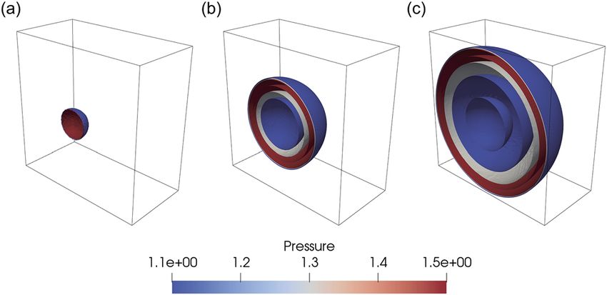
To demonstrate the evolution process of the spherical explo-
sion, we choose several typical snapshots of the pressure isosurfaces
at various times in Fig. 7. Since the computational system is sym-
metrical, only half of the system is depicted for clear illustration.
Figure 7(a) shows the initial configuration, and (b) and (c) display FIG. 7. Snapshots of the pressure isosurfaces in the spherical explosion process:
(a) t = 0, (b) t = 0.0025, and (c) t = 0.005.
the evolution process at time t = 0.0025 and 0.005, respectively. First,
AIP Advances 11, 045217 (2021); doi: 10.1063/5.0047480 11, 045217-10
© Author(s) 2021AIP Advances ARTICLE scitation.org/journal/adv
FIG. 8. The temporal histories of physical quantities. (a) Density; (b) internal, kinetic, chemical, and total energies.
energies remains unchanged. Figure 8 indicates that the mass and from the UK Engineering and Physical Sciences Research Coun-
energy of the system are conserved. It is shown that the proposed cil under the project UK Consortium on Mesoscale Engineering
DBM has a satisfying performance for simulations of 3D reacting Sciences (UKCOMES) (Grant No. EP/R029598/1) is also gratefully
flows. acknowledged.
V. CONCLUSION APPENDIX: TRANSFORMATION MATRIX AND KINETIC
MOMENTS
In this paper, a 3D MRT DBM is presented for reactive flows
where both the Prandtl number and specific heat ratio are freely The equilibrium distribution function is
adjustable. There are 30 kinetic moments of discrete distribution
functions, and an efficient discrete velocity model, D3V30, is uti- m D/2 m 1/2 m∣v − u∣2 mη2
f eq = ρ( ) ( ) exp[− − ]. (A1)
lized. The NS equations can be recovered at macroscales from the 2πT 2πIT 2T 2IT
DBM through the Chapman–Enskog analysis. Unlike existing LBMs
for reactive flows, the hydrodynamic and thermodynamic fields are The transformation matrix reads
fully coupled in the DBM to simulate combustion in subsonic, super-
sonic, and potentially hypersonic flows. In addition, the nonequi- M = (M1i , M1i , . . . , M30i )⊺ , (A2)
librium effects of the system can be probed and quantified. In this
with elements M 1i = 1, M 2i = vix , M 3i = viy , M 4i = viz , M5i = vix 2
+ viy2
model, the reaction and force terms added into the discrete Boltz-
mann equation describe the change rates of discrete functions due + viz + ηi , M 6i = vix vix , M 7i = viy viy , M 8i = viz viz , M 9i = vix viy , M 10i
2 2
to the chemical heat release and external force, respectively. = vix viz , M 11i = viy viz , M12i = (vix 2
+ viy2 + viz2 + η2i )vix , M13i = (vix
2
The DBM has been validated for several typical applications. + viy + viz + ηi )viy , M14i = (vix + viy + viz + ηi )viz , M 15i = vix vix vix ,
2 2 2 2 2 2 2
The capability of the DBM to simulate the flow field fully cou- M 16i = vix vix viy , M 17i = vix vix viz , M 18i = vix viy viy , M 19i = vix viy viz ,
pled with a chemical reaction and external force is verified using M 20i = vix viz viz , M 21i = viy viy viy , M 22i = viy viy viz , M 23i = viy viz viz ,
the free falling reacting box. The case of the thermal Couette flow M 24i = viz viz viz , M25i = (vix2
+ viy2 + viz2 + η2i )vix vix , M26i = (vix2
+ viy2
demonstrates that both the specific heat ratio and Prandtl number + viz + ηi )vix viy , M27i = (vix + viy + viz + ηi )vix viz , M28i = (vix + viy2
2 2 2 2 2 2 2
are adjustable. Furthermore, the DBM is shown to accurately sim- + viz2 + η2i )viy viy , M29i = (vix
2
+ viy2 + viz2 + η2i )viy viz , and M30i = (vix 2
ulate supersonic flows and quantify the nonequilibrium effects in
1D detonation. Finally, the main features of a spherical explosion + viy + viz + ηi )viz viz .
2 2 2
in an enclosed box are successfully captured to showcase the ability According to Eq. (3), the kinetic moments of the discrete
of the DBM to deal with a 3D configuration. In conclusion, a new equilibrium distribution function take the following forms:
eq ⊺
3D DBM for reactive flows featuring full coupling of flow and com- eq eq
bustion fields has been developed and successfully validated. This f̂ eq = (f̂ 1 , f̂ 2 , . . . , f̂ 30 ) , (A3)
opens up possibilities for exploring a variety of reactive flows at sub-
eq eq eq eq eq
sonic, supersonic, and hypersonic speeds with both hydrodynamic with elements f̂ 1 = ρ, f̂ 2 = ρux , f̂ 3 = ρuy , f̂ 4 = ρuz , f̂ 5 = ρ[(D + I)
eq eq eq eq
and thermodynamic nonequilibria. T + u2 ], f̂ 6 = ρ(T + u2x ), f̂ 7 = ρ(T + u2y ), f̂ 8 = ρ(T + u2z ), f̂ 9
eq eq eq eq
= ρux uy , f̂ 10 = ρux uz , f̂ 11 = ρuy uz , f̂ 12 = ρux [(D + I + 2)T + u2 ], f̂ 13
eq eq
ACKNOWLEDGMENTS = ρuy [(D + I + 2)T + u2 ], f̂ 14 = ρuz [(D + I + 2)T + u2 ], f̂ 15 = ρ(3ux
eq eq eq
T + u3x ), f̂ 16 = ρ(uy T + u2x uy ), f̂ 17 = ρ(uz T + u2x uz ), f̂ 18 = ρ(ux T
This work was supported by the National Natural Science eq eq eq
Foundation of China (NSFC) under Grant No. 51806116 and the + ux uy ), f̂ 19 = ρux uy uz , f̂ 20 = ρ(ux T + ux uz ), f̂ 21 = ρ(3uy T + u3y ),
2 2
eq eq eq
Center for Combustion Energy at Tsinghua University. Support f̂ 22 = ρ(uz T + uz u2y ), f̂ 23 = ρ(uy T + uy u2z ), f̂ 24 = ρ(3uz T + u3z ),
AIP Advances 11, 045217 (2021); doi: 10.1063/5.0047480 11, 045217-11
© Author(s) 2021AIP Advances ARTICLE scitation.org/journal/adv
eq eq
f̂ 25 = ρT[(D + I + 2)T + u2 ] + ρu2x [(D + I + 4)T + u2 ], f̂ 26 = ρux uy 5
A. Munafò, M. Panesi, and T. E. Magin, “Boltzmann rovibrational collisional
eq eq coarse-grained model for internal energy excitation and dissociation in hypersonic
[(D + I + 4)T + u2 ], f̂ 27 = ρux uz [(D + I + 4)T + u2 ], f̂ 28 = ρT[(D
eq flows,” Phys. Rev. E 89, 023001 (2014).
+ I + 2)T + u ] + ρuy [(D + I + 4)T + u ], f̂ 29 = ρuy uz [(D + I + 4)T
2 2 2
6
Y. Ju, “Recent progress and challenges in fundamental combustion research,”
eq
+ u2 ], and f̂ 30 = ρT[(D + I + 2)T + u2 ] + ρu2z [(D + I + 4)T + u2 ]. Adv. Appl. Mech. 44, 201402 (2014).
7
The force term reads N. Gebbeken, S. Greulich, and A. Pietzsch, “Hugoniot properties for concrete
determined by full-scale detonation experiments and flyer-plate-impact tests,” Int.
⊺ J. Impact Eng. 32, 2017–2031 (2006).
F̂ = (F̂ 1 , F̂ 2 , . . . , F̂ 30 ) , (A4) 8
J. A. T. Gray, M. Lemke, J. Reiss, C. O. Paschereit, J. Sesterhenn, and J. P.
Moeck, “A compact shock-focusing geometry for detonation initiation: Exper-
iments and adjoint-based variational data assimilation,” Combust. Flame 183,
with elements F̂ 1 = 0, F̂ 2 = ρax , F̂ 3 = ρay , F̂ 4 = ρaz , F̂ 5 = 2ρ(ux ax 144–156 (2017).
+ uy ay + uz az ), F̂ 6 = 2ρux ax , F̂ 7 = 2ρuy ay , F̂ 8 = 2ρuz az , F̂ 9 = ρ(ux ay 9
S. T. Parete-Koon, C. R. Smith, T. L. Papatheodore, and O. E. Bronson Messer,
+ uy ax ), F̂ 10 = ρ(ux az + uz ax ), F̂ 11 = ρ(uy az + uz ay ), F̂ 12 = 2ρux “A review of direct numerical simulations of astrophysical detonations and their
(ux ax + uy ay + uz az ) + ρax [(D + I + 2)T + u2 ], F̂ 13 = 2ρuy (ux ax implications,” Front. Phys. 8, 189–198 (2013).
10
Y. Mahmoudi, N. Karimi, R. Deiterding, and S. Emami, “Hydrodynamic insta-
+ uy ay + uz az ) + ρay [(D + I + 2)T + u2 ], F̂ 14 = 2ρuz (ux ax + uy ay bilities in gaseous detonations: Comparison of Euler, Navier–Stokes, and large-
+ uz az ) + ρaz [(D + I + 2)T + u2 ], F̂ 15 = 3ρax (T + u2x ), F̂ 16 = ρ[ay eddy simulation,” J. Propul. Power 30, 384–396 (2014).
(T + u2x ) + 2ax ux uy ], F̂ 17 = ρ[az (T + u2x ) + 2ax ux uz ], F̂ 18 = ρ[ax (T 11
B. M. Haines, F. F. Grinstein, and J. D. Schwarzkopf, “Reynolds-averaged
+ u2y ) + 2ay ux uy ], F̂ 19 = ρ[ax uy uz + ay ux uz + az uy ux ], F̂ 20 = ρ[ax (T Navier–Stokes initialization and benchmarking in shock-driven turbulent
mixing,” J. Turbul. 14, 46–70 (2013).
+ u2z ) + 2az ux uz ], F̂ 21 = 3ρay (T + u2y ), F̂ 22 = ρ[az (T + u2y ) + 2 12
Y. Zhang, R. Qin, and D. R. Emerson, “Lattice Boltzmann simulation of rarefied
ay uy uz ], F̂ 23 = ρ[ay (T + uz ) + 2az uy uz ], F̂ 24 = 3ρaz (T + u2z ), F̂ 25
2
gas flows in microchannels,” Phys. Rev. E 71, 047702 (2005).
= 2ρ(ux ax + uy ay + uz az )(T + u2x ) + 2ρux ax [(D + I + 4)T + u2 ], F̂ 26 13
J. Meng, Y. Zhang, N. G. Hadjiconstantinou, G. A. Radtke, and X. Shan, “Lattice
= 2ρ(ux ax + uy ay + uz az )ux uy + ρ(ux ay + uy ax )[(D + I + 4)T + u2 ], ellipsoidal statistical BGK model for thermal non-equilibrium flows,” J. Fluid
Mech. 718, 347–370 (2013).
F̂ 27 = 2ρ(ux ax + uy ay + uz az )ux uz + ρ(ux az + uz ax )[(D + I + 4)T 14
V. V. Zhakhovskii, K. Nishihara, and S. I. Anisimov, “Shock wave structure in
+ u2 ], F̂ 28 = 2ρ(ux ax + uy ay + uz az )(T + u2y ) + 2ρuy ay [(D + I + 4)T dense gases,” JETP Lett. 66, 99–105 (1997).
+ u2 ], F̂ 29 = 2ρ(ux ax + uy ay + uz az )uy uz + ρ(uy az + uz ay )[(D + I 15
B. L. Holian, C. W. Patterson, M. Mareschal, and E. Salomons, “Modeling shock
+ 4)T + u2 ], and F̂ 30 = 2ρ(ux ax + uy ay + uz az )(T + u2z ) + 2ρuz az waves in an ideal gas: Going beyond the Navier–Stokes level,” Phys. Rev. E 47,
R24–R27 (1993).
[(D + I + 4)T + u2 ]. 16
B. L. Holian and M. Mareschal, “Heat-flow equation motivated by the ideal-gas
The reaction term is shock wave,” Phys. Rev. E 82, 026707 (2010).
17
A. V. Bobylev, M. Bisi, M. P. Cassinari, and G. Spiga, “Shock wave structure for
⊺
R̂ = (R̂1 , R̂2 , . . . , R̂30 ) , (A5) generalized Burnett equations,” Phys. Fluids 23, 030607 (2011).
18
S. Succi, The Lattice Boltzmann Equation: For Complex States of Flowing Matter
(Oxford University Press, 2018).
with elements R̂1 = 0, R̂2 = 0, R̂3 = 0, R̂4 = 0, R̂5 = (D + I)ρT ′ , 19
S. Succi, G. Bella, and F. Papetti, “Lattice kinetic theory for numerical
R̂6 = ρT ′ , R̂7 = ρT ′ , R̂8 = ρT ′ , R̂9 = 0, R̂10 = 0, R̂11 = 0, R̂12 = (D combustion,” J. Sci. Comput. 12, 395–408 (1997).
+ I + 2)ρux T ′ , R̂13 = (D + I + 2)ρuy T ′ , R̂14 = (D + I + 2)ρuz T ′ , R̂15
20
O. Filippova and D. Hänel, “A novel lattice BGK approach for low Mach number
= 3ρux T ′ , R̂16 = ρuy T ′ , R̂17 = ρuz T ′ , R̂18 = ρux T ′ , R̂19 = 0, R̂20 combustion,” J. Comput. Phys. 158, 139–160 (2000).
= ρux T ′ , R̂21 = 3ρuy T ′ , R̂22 = ρuz T ′ , R̂23 = ρuy T ′ , R̂24 = 3ρuz T ′ , R̂25
21
O. Filippova and D. Häenel, “A novel numerical scheme for reactive flows at low
Mach numbers,” Comput. Phys. Commun. 129, 267–274 (2000).
= [2(D + I + 2)T + u2 + (D + I + 4)u2x ]ρT ′ , R̂26 = ρT ′ ux uy (D + I 22
S. A. Hosseini, A. Eshghinejadfard, N. Darabiha, and D. Thévenin, “Weakly
′
+ 4), R̂27 = ρT ux uz (D + I + 4), R̂28 = [2(D + I + 2)T + u2 + (D + I compressible lattice Boltzmann simulations of reacting flows with detailed
+ 4)u2y ]ρT ′ , R̂29 = ρT ′ uy uz (D + I + 4), and R̂30 = [2(D + I + 2)T thermo-chemical models,” Comput. Math. Appl. 79, 141–158 (2020).
+ u2 + (D + I + 4)u2z ]ρT ′ .
23
S. A. Hosseini, H. Safari, N. Darabiha, D. Thévenin, and M. Krafczyk, “Hybrid
lattice Boltzmann-finite difference model for low Mach number combustion
simulation,” Combust. Flame 209, 394–404 (2019).
24
Y. Peng, C. Shu, and Y. T. Chew, “Simplified thermal lattice Boltzmann model
DATA AVAILABILITY for incompressible thermal flows,” Phys. Rev. E 68, 026701 (2003).
25
The data that support the findings of this study are available K. Yamamoto, X. He, and G. D. Doolen, “Simulation of combustion field with
from the corresponding author upon reasonable request. lattice Boltzmann method,” J. Stat. Phys. 107, 367–383 (2002).
26
K. Yamamoto, “LB simulation on combustion with turbulence,” Int. J. Mod.
Phys. B 17, 197–200 (2008).
27
REFERENCES T. Lee, C. Lin, and L. Chen, “A lattice Boltzmann algorithm for calculation of
the laminar jet diffusion flame,” J. Comput. Phys. 215, 133–152 (2006).
1
C. K. Law, Combustion Physics (Cambridge University Press, Cambridge, 28
S. Chen, Z. Liu, C. Zhang, Z. He, Z. Tian, B. Shi, and C. Zheng, “A novel coupled
2006). lattice Boltzmann model for low Mach number combustion simulation,” Appl.
2
See https://yearbook.enerdata.net/total-energy/world-consumption-statistics. Math. Comput. 193, 266–284 (2007).
html for trend over 1990-2019, in global energy statistical yearbook 2020. 29
S. Chen, Z. Liu, Z. Tian, B. Shi, and C. Zheng, “A simple lattice Boltzmann
3
E. Nagnibeda and E. Kustova, Non-Equilibrium Reacting Gas Flows: Kinetic scheme for combustion simulation,” Comput. Math. Appl. 55, 1424–1432 (2008).
Theory of Transport and Relaxation Processes (Springer, Berlin, 2009). 30
A. F. di Rienzo, P. Asinari, E. Chiavazzo, N. I. Prasianakis, and J. Mantzaras,
4
E. V. Kustova and D. Giordano, “Cross-coupling effects in chemically non- “Lattice Boltzmann model for reactive flow simulations,” Europhys. Lett. 98,
equilibrium viscous compressible flows,” Chem. Phys. 379, 83–91 (2011). 34001 (2012).
AIP Advances 11, 045217 (2021); doi: 10.1063/5.0047480 11, 045217-12
© Author(s) 2021AIP Advances ARTICLE scitation.org/journal/adv
31 46
B. Yan, A. Xu, G. Zhang, Y. Ying, and H. Li, “Lattice Boltzmann model for H. Lai, A. Xu, G. Zhang, Y. Gan, Y. Ying, and S. Succi, “Non-equilibrium
combustion and detonation,” Front. Phys. 8, 94–110 (2013). thermo-hydrodynamic effects on the Rayleigh-Taylor instability in compressible
32 flows,” Phys. Rev. E 94, 023106 (2016).
C. Lin, A. Xu, G. Zhang, and Y. Li, “Polar coordinate lattice Boltzmann
47
kinetic modeling of detonation phenomena,” Commun. Theor. Phys. 62, 737–748 T. Kataoka and M. Tsutahara, “Lattice Boltzmann model for the compressible
(2014). Navier-Stokes equations with flexible specific-heat ratio,” Phys. Rev. E 69, 35701
33
A. Xu, C. Lin, G. Zhang, and Y. Li, “Multiple-relaxation-time lattice Boltzmann (2004).
48
kinetic model for combustion,” Phys. Rev. E 91, 043306 (2015). M. Watari and M. Tsutahara, “Two-dimensional thermal model of the finite-
34
C. Lin, A. Xu, G. Zhang, and Y. Li, “Double-distribution-function dis- difference lattice Boltzmann method with high spatial isotropy,” Phys. Rev. E 67,
crete Boltzmann model for combustion,” Combust. Flame 164, 137–151 036306 (2003).
49
(2016). M. Watari, “Is the lattice Boltzmann method applicable to rarefied gas flows?
35
C. Lin and K. H. Luo, “Mesoscopic simulation of nonequilibrium detonation Comprehensive evaluation of the higher-order models,” J. Fluids Eng. 138, 011202
with discrete Boltzmann method,” Combust. Flame 198, 356–362 (2018). (2016).
36 50
C. Lin and K. H. Luo, “Discrete Boltzmann modeling of unsteady reactive flows F. Chen, A. Xu, G. Zhang, Y. Li, and S. Succi, “Multiple-relaxation-time lattice
with nonequilibrium effects,” Phys. Rev. E 99, 012142 (2019). Boltzmann approach to compressible flows with flexible specific-heat ratio and
37 Prandtl number,” Europhys. Lett. 90, 54003 (2010).
T. Yang, J. Wang, L. Yang, and C. Shu, “Development of multi-component
51
generalized sphere function based gas-kinetic flux solver for simulation of com- Y. Zhang, A. Xu, G. Zhang, C. Zhu, and C. Lin, “Kinetic modeling of detonation
pressible viscous reacting flows,” Comput. Fluids 197, 104382 (2020). and effects of negative temperature coefficient,” Combust. Flame 173, 483–492
38 (2016).
S. Ansumali and I. V. Karlin, “Consistent lattice Boltzmann method,” Phys. Rev.
52
Lett. 95, 260605 (2005). C. Shu and S. Osher, “Efficient implementation of essentially non-oscillatory
39
C. Lin and K. H. Luo, “MRT discrete Boltzmann method for compressible shock-capturing schemes,” J. Comput. Phys. 77, 439–471 (1989).
53
exothermic reactive flows,” Comput. Fluids 166, 176–183 (2018). H. D. Ng, M. I. Radulescu, A. J. Higgins, N. Nikiforakis, and J. H. S.
40
T. Ruggeri and M. Sugiyama, Rational Extended Thermodynamics Beyond the Lee, “Numerical investigation of the instability for one-dimensional Chapman–
Monatomic Gas (Springer, 2015). Jouguet detonations with chain-branching kinetics,” Combust. Theory Modell. 9,
41 385–401 (2005).
T. Ruggeri, “Maximum entropy principle closure for 14-moment system for a
54
non-polytropic gas,” Ric. Mat. 2020, 1–16. W. Fickett and W. W. Wood, “Flow calculations for pulsating one-dimensional
42 detonations,” Phys. Fluids 9, 903–916 (1966).
Y. Gan, A. Xu, G. Zhang, and H. Lai, “Three-dimensional discrete Boltzmann
55
models for compressible flows in and out of equilibrium,” Proc. Inst. Mech. Eng., H. I. Lee and D. S. Stewart, “Calculation of linear detonation instability: One-
Part C 232, 477–490 (2018). dimensional instability of planer detonations,” J. Fluid Mech. 216, 103–132 (1990).
43 56
S. Chen, H. Chen, D. Martnez, and W. Matthaeus, “Lattice Boltzmann A. Bourlioux and A. J. Majda, “Theoretical and numerical structure for unstable
model for simulation of magnetohydrodynamics,” Phys. Rev. Lett. 67, 3776 one-dimensional detonations,” Combust. Flame 90, 211–229 (1992).
57
(1991). Z. Gao, W. Don, and Z. Li, “High order weighted essentially non-oscillation
44
Y. H. Qian, D. D’Humières, and P. Lallemand, “Lattice BGK models for schemes for one-dimensional detonation wave simulations,” J. Comput. Math. 29,
Navier–Stokes equation,” Europhys. Lett. 17, 479 (1992). 623 (2011).
45 58
J. Bourgat, L. Desvillettes, P. Tallec, and B. Perthame, “Microreversible colli- C. Wang, P. Li, Z. Gao, and W. Don, “Three-dimensional detonation simula-
sions for polyatomic gases and Boltzmann’s theorem,” Eur. J. Mech. B 13, 237–254 tions with the mapped WENO-Z finite difference scheme,” Comput. Fluids 139,
(1994). 105–111 (2016).
AIP Advances 11, 045217 (2021); doi: 10.1063/5.0047480 11, 045217-13
© Author(s) 2021You can also read