THOMAS JEFFERSON PHYSICS OLYMPIAD - TJPHO - ACTIVITIES
←
→
Page content transcription
If your browser does not render page correctly, please read the page content below
4rd Annual TJPhO — 2022-05-13                                                           TJPhO

                   Thomas Jefferson Physics Olympiad
                                    A high school physics contest

                             TJ Physics Team

                                  The James Webb Space Telescope

                 If you have any questions or concerns, please email TJ Physics Team.
Contents

Rules                                        3

Introduction                                 5

The James Webb Space Telescope (JWST)        7

Imaging in The James Webb Space Telescope   10

Additional Assorted Problems                13

Coding Problems                             19

Additional Resources                        22

                               Page 2
Rules

Teams will have from 9:00 PM EST on March 13th to 9:00 PM EST on Marth 15th to
complete the TJPhO. All teams are required to submit their response with a cover page
listing the team name and number, team member names, team email, and the date. Each
submitted page should also have the problem number. All other formatting decisions are
delegated to the teams themselves, with no one style favored over another. We suggest
that teams use LATEX for typesetting. The easiest way we’ve found to typeset LATEX is
with Overleaf.

Problems

Many of our problems will focus on the James Webb Space Telescope and the foundational
physics that went into designing it. There is also a wild card section which has questions
on an assortment of different topics – it is up to you to decide what approach you need
to use. Lastly, we have a coding section, where in addition to doing some math you are
expected to write a program in a language of your choice and submit your code for us to
review.

Our problems were written by Tarushii Goel, Cyril Sharma, Anya Mischel, and Alvan
Caleb Arlandu. We would like to thank Dr. Jonathan Osborne for reviewing our problems
and providing valuable feedback.

Collaboration

Students participating in the competition may only correspond with other members of
their team. No other correspondence is allowed, including mentors, teachers, professors,
and other students. Teams are not allowed to use online/print resources or post content
on online forums asking questions related to the exam. We welcome teams to email
us if there are any questions or concerns. If a problem explicitly states that it is
allowed, teams may use computational resources they might find helpful, such as Wolfram
Alpha/Mathematica, Matlab, Excel, or programming languages.

Submission

Teams must submit their solutions by email to tjhsstphysicsteam@gmail.com by the
deadline 9:00 PM EST on May 15th. Late submissions will not be considered. Solutions
should be written in English and submitted as a single PDF document with the .pdf

                                         Page 3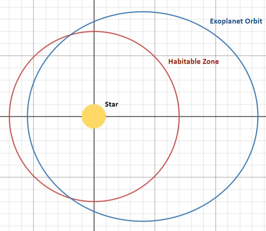
extension. The email must contain “Submission” in the subject line. Only one person
per team, the person who registered through the Google Form, should send the final
submission.

Awards

The top five teams will receive awards.

1st place: $200, 3 one-year subscriptions to WolframAlpha Notebook Edition

2nd place: $150, 3 one-year subscriptions to WolframAlpha Notebook Edition

3rd place: $100, 3 one-year subscriptions to WolframAlpha Notebook Edition

4/5th place: 3 one-year subscriptions to WolframAlpha Notebook Edition

Sponsors

We are incredibly grateful to our sponsors, Dr. Adam Smith and Mr. Robert Culbertson,
and Thomas Jefferson High School for Science and Technology for their support. We
would also like thank our sponsors WolframAlpha and the Thomas Jefferson Partnership
Fund for making this Olympiad possible.

                                          Page 4
Introduction
The James Webb Space Telescope (JWST) was developed in a collaboration between
NASA, the European Space Agency (ESA), and the Canadian Space Agency. It is
named after James E. Webb, who was the administrator of NASA from 1961 to 1968.
Development began in 1996 on a $500 million budget with a launch initially planned for
2007. Instead it was launched last year and costed an esitmated total of $9.7 billion.
Figure 1: The James Webb Space Telescope
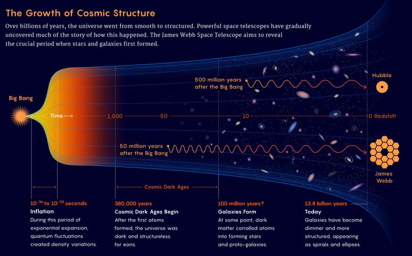
It is designed to perform near-infrared astronomy and is capable of seeing objects that
are too faint and distant for the Hubble Space Telescope to capture images of. It can see
as far back as 50 million years after the Big Bang.
Figure 2: History of the Universe
Page 5The JWST was launched along with the Ariane 5 rocket on December 25th, 2021, from a
ESA launch site in French Guiana. On December 27th, it sailed beyond the orbit of the
moon, and on December 31st, it began the process of unfurling its massive sun shield and
tightening the layers, a process that took until January 3rd, 2022. On January 24th, it
finally arrived at the second lagrange point, L2, where it will remain while it takes high
resolution images of space (previously, the Herschel Space Telescope and Planck Space
Observatory have also orbited at the L2 point). The JWST has finished unfolding its
mirrors and has spent the last few months aligning its optical instruments. Just a few
days ago, it reached the end of its alignment process and took a high resolution image,
which is included in Figure 4.
Figure 3: The first image taken by the JWST, at the beginning of the long process of
alignment. THe light is from a star named HD84406. Each of the 18 bright dots is
the light reflected by one of the JWST’s 18 primary mirror segments. (Image credit:
NASA/ESA/CSA/STScI)
Figure 4: The Large Magellanic Cloud, as seen by NASA’s Spitzer Space Telescope (left)
and the JWST after a long period of alignement (right). (Image credit: NASA/JPL-
Caltech (left), NASA/ESA/CSA/STScI (right))
Page 6The James Webb Space Telescope (JWST)
1. Lagrange Points. When communicating with a satellite, it’s desirable if the satellite
is always in the same place. Lagrange points are thus an attractive destination for
satellites; as they remain stationary relative to the Earth (they orbit the sun with
the same angular velocity as Earth). For this reason, the JWST has been sent to
orbit the second Lagrange point, shown below.
S
L2
D
Figure 5: Langrange Point
(a) (1 point) Calculate the distance to L2, D, in terms of the mass of the earth and
sun, Me and Ms , and the distance of the sun from the earth, S. Hint: L2 does
not move relative to the Earth, meaning it orbits the sun with the same angular
velocity as the Earth.
(b) (1 point) Calculate the gravitational potential energy as a function of the
distance from the sun in the direction of the earth. You may assume the Earth
and Sun are point masses. The JWST has mass mj .
(c) (1 point) The potential function calculated above doesn’t account for the
centripetal force needed to stay in the same relative position. Pick a frame
of reference that rotates around the sun with the earth. From this frame of
reference, a centrifugal force acts on all bodies away from the axis of rotation.
Compute the effective potential function, a potential function that takes into
account both the centrifugal force and the gravitational forces.
(d) (1 point) Contrary to the calculated potential function, L2 is actually fairly easy
to orbit. This is because the Coriolis force helps stabilize L2 orbits. The diagram
below shows how the Coriolis force and gravitational forces balance, allowing an
object to stay in a stable orbit around L2. Qualitatively explain how an object
moved slightly towards the Earth from its spot on L2 would find itself at this
steady state in terms of the Coriolis and gravitational forces.
Page 7Coriolis Force
Gravity
θ
Figure 6: Stable Orbit of Lagrange Point
(e) (1 point) Let the distance between the Earth and the Sun be S. Let the distance
along the x axis from the Earth to the JWST be D. You may assume the sun’s
gravitational pull is not significantly angled, and is directed purely in x direction,
as shown in the diagram. In terms of S and D, what angle θ must the JWST be
at relative to the Earth in order to remain stationary relative to the Earth?
y
Sun x
θ
D
Figure 7
2. Solar Radiation Effects. The JWST’s sensitive infrared imaging technology must be
Page 8kept at low temperatures to operate correctly. For this reason, the JWST has a sun
shield made of Kapton E that blocks solar radiation. We can model the sun shield
as a flat surface being struck by electromagnetic (EM) waves.
The energy flux of an EM wave is known as the Poynting vector, S. This fluctuates
with the frequency of the EM wave, but generally all we care about is the average of
the magnitude of the Poynting vector, ⟨S⟩, which is also known as the light irradiance,
S
I. The momentum density of EM waves is P = 2 . For this problem, assume that
c
the Poynting vector is perpendicular to the shield.
(a) (1 point) Express the average pressure pa exerted on the sun shield as a function
of I and c, assuming the shield absorbs 100% of the radiation. Then calculate
the pressure pr when it perfectly reflects the radiation.
(b) (1 point) The shield is 22 by 10 m in size, its reflectance factor is 0.8, and the
irradiance of light at the L2 point, where the JWST is situated, is about 1366
W/m2 (this is actually the irradiance of light at the Earth, but the L2 point is
only 0.01 AU away so the difference is negligible). Calculate the total force solar
radiation exerts on the shield.
(c) (2 points) Random fluctuations in solar irradiance can cause pressure gradients
across the sun shield, which result in a torque. Use the set up shown below,
where the force calculated in the previous question is directed towards the very
end of the shield rather than evenly distributed, to calculate the torque on the
shield. The effects of this torque need to be mitigated in order to keep the shield
facing the sun and protect the JWST’s sensitive equipment. One approach of
doing so is to use a momentum wheel with stored angular momentum. Using
the set up shown below, where the torque you calculated is exerted on the
momentum wheel for a period of one day, to find the total rotation θ in terms of
the angular momentum L of the momentum wheel, which is directed downwards
on the figure below (IW >> IS , where IW and IS are of moments of inertia about
the COM of the wheel and shield for the wheel and shield, respectively). Graph
θ vs. L. What is the axis of rotation?
Figure 8: Top View of Shield-Wheel Configuration
3. (5 points) Exoplanets. Suppose the JWST discovers a faraway exoplanet orbiting
a star in an elliptical orbit with eccentricity 0.42 and a semi-major axis of 1.9 AU.
In order for this particular planet to have the possibility of carbon-based life, the
Page 9planet spend at least 20% of the time of its orbit within 1.4 AU of the star. Given
this information, does the planet stay within the maximum habitability distance long
enough to have the possibility to support life? Wolfram Alpha or other integration-
solving software is permitted for this problem only, but all steps including the integral
expression must be explicitly written.
Figure 9: Exoplanet Orbit and Habitability Boundary
Imaging in the James Webb Space Telescope
4. Lenses. Lenses rely on the law of refraction, which states that light will bend when
transitioning between two media. Specifically, n1 sin θ1 = n2 sin θ2 , where n1 and n2
are the indices of refraction of the materials (phase speed v = c/n), and θ1 and θ2 are
the angles that the incident and transmitted light rays make with the perpendicular
to the boundary between the materials. JWST’s lenses use refraction to concentrate
light onto a focal point, thereby creating high resolution images.
Page 10Figure 10: Refraction of Light Passing Through Different Materials
(a) (3 points) Suppose you have a lens as shown in the setup below (gray region is
glass), which focuses light from point source S in space at focal point P inside
the lens. According to Fermat’s principle of least time, both light rays shown
must take the same amount of time to travel between the two points. By relating
the travel times of the two rays, establish a relationship between s1 and s2 in
terms of R, the radius of the lens, n1 , and n2 . Assume d21 − s21 = (d1 − s1 )2s1 ,
d22 − s22 = (d2 − s2 )2s2 , and R2 − x2 = (R − x)2R.
Figure 11: A Lens
(b) (2 points) Replace the lens used in the previous question with a lens of the shape
shown in the figure below, and derive a new expression relating s1 and s2 , in
terms of R1 , R2 , n1 , and n2 . Assume dFigure 12: A Thin Lens
(c) (1 point) Generally, the sources of light which a lens is engineered to focus are
much farther away than from the lens than the focal points of those sources of
light (e.g. the JWST images stars many light years away but the star image
may be constructed a few centimeters away). The distance at which the image
focuses is the f , the focal length, which is derived by letting s1 = ∞. Plug this
value for s1 into you answer for the previous part to find the focal length.
(d) (1 point) Light waves warp while traveling through space, and being able to
measure these distortions and adapt optical systems accordingly is crucial. One
method of measuring wavefront distortions is to arrange lenslets in a line, as
shown in the figure below. Each lenslet will focus light on a different point on
the image plane (see figure below), due to the difference in the angle at which
the wavefront strikes the lens. Demonstrate how the lenslet array distinguishes
between different wavefronts by marking the focal point of each lenslet for a
planar wavefront. Then mark the focal points for the distorted wavefront, which
may be shifted up or down. You should draw a total of 10 points, 5 on each
image plane.
Figure 13: A Lenslet Array
5. Diffraction. The JWST’s optical equipment is precisely fine-tuned so as to produce
the highest resolution images possible. However, the resolution of these images has
a theoretical limit due to the diffraction of light.
Page 12(a) (3 points) Let’s say you have a line of n harmonic electron oscillators spaced by a
distance d that are moving in phase. The electric field created by single oscillator
2πr
at a large distance r away from can be approximated as A cos (wt − ), where
λ
λ is the wavelength of electromagnetic wave, and w is its angular velocity. Write
the resultant amplitude of the field oscillation AR at a point a distance r away
and at an angle θ (in terms of A, f , the frequency of oscillation, d, and θ).
Note that in the diagram below the light rays reaching the point are shown as
approximately parallel (and you can assume they are) because the point is very
far away.
Figure 14: Electron Oscillator Setup where n = 5
(b) (1 point) Plot I (the light irradiance, which is explained in the solar radiation
problem) vs. θ. At what values of θ do you see the greatest irradiance of light?
Where is the irradiance 0?
(c) (1 point) Let’s think of a one of the JWST’s lenses as a small, circular opening
in a barrier that allows light to pass through. The theory of diffraction states
that the light passing through the opening is equivalent to that which would
be generated by a lot of (really, infinitely many) sources of light of the same
wavelength evenly separated by a small distance across the opening. So, the
light that passes through the opening forms a diffraction pattern that is quite
similar to that which you calculated in previous parts. Draw the diffraction
pattern you would expect (it does not have to be mathematically precise, we
are only looking for the general position of high irradiance and low irradiance
regions).
Interestingly, the angle θ at which the first minimum in light irradiance occurs,
measured from the direction of incoming light, is approximated by the formula
λ
sin θ = 1.22 where d is the diameter of the aperture. So, using the Raleigh Criterion,
d
θ is the smallest angular separation you can have between two objects while still being
able to resolve them. This is what we mean when we say that the resolution of a
camera is diffraction-limited.
Additional Assorted Problems
6. Windmills.
Page 13(a) (1 point) Windmills generate energy by slowing down the wind and extracting
its energy. Suppose we have a windmill as shown in the figure below. Assuming
that we are dealing with incompressible, irrotational, and steady flow of air,
which of the colored lines (red, blue, or black) best represents the general shape
of the streamtube of air that passes through the windmill?
Figure 15: Top View of a Windmill
(b) (2 points) Bernoulli’s equation, which is derived from conservation of energy,
1
states that P + ρv 2 + ρgh is remains constant in steady flow. Assuming
2
that energy is not inputted or outputted into the streamtube upstream or
downstream of the windmill (only at the windmill), apply Bernoulli’s equation
to find the force exerted on the windmill. Express you answer in terms of W , the
undisturbed wind speed, Aw , the area of the windmill, ρ, the density of air, and a,
the induction factor, which is related to the design of the windmill and indicates
much energy it extracts (specifically, the speed of air at the windmill is W (1−a)),
and the unknown W∞ , which is the speed of the air far downstream. Assume
that gravitational potential energy is unchanging during fluid flow. Additionally,
draw graphs of the pressure and wind speed vs. position along the streamtube
(these only need to be correct to the first derivative).
(c) (1 point) Derive another expression for the force on the windmill, this time
applying conservation of momentum (in terms of the same variables as the
previous part).
(d) (1 point) Combine the expressions you found in the last two parts to find W∞
in terms of W
(e) (1 point) Plug your expression for W∞ back in to get a formulation for power
extracted (assume 100% efficiency). What induction factor gives you the highest
power? What is the ratio between the maximum power you can extract and the
power of the wind passing through the windmill?
(f) (1 point) Now let’s consider a contraption composed of two propellers, one in
the air and one in the water, connected by a shaft, as shown in the figure below.
The analysis for the the force on power extracted by the propeller in the air
is exactly the same as that established in the previous parts. However, the
propeller in the water must be reanalyzed (though the steps to do so are very
similar) because it functions more like a fan than a windmill, speeding up the
Page 14water to a speed V at the propeller. Calculate the power delivered by the water
propeller to the water in terms of ρ2 , A2 , V .
Figure 16: Propeller Contraption
(g) (1 point) Assume Pin = Pout , and calculate the net force on the contraption
using the induction factor that provides maximum efficiency (calculated in a
previous part). You answer should be in terms of a subset of these variables:
ρ1 , A1 , ρ2 , A2 , W .
(h) (2 points) What is the maximum speed of this contraption, in terms of W ? (the
answer may be surprising)
7. Ceaseless Cylinders. Two infinitely long concentric cylindrical conducting shells are
grounded (this means that they are connected to an infinite source/sink of charge,
and charge can be induced on the conductors in order to maintain a potential of 0).
The outermost conductor (conductor B) has a radius b, and the innermost conductor
(conductor A) has a radius a. A single point charge q is place at some radius r
(a < r < b), inducing charge on the conductors (QA and QB ).
(a) (1 point) What is the total charge induced on both conductors, QA + QB ?
(in terms of some subset of the following variables: a, b, q, r). Provide a short
explanation for how you can determine this without knowing QA or QB .
(b) (6 points) Green’s reciprocity theorem states that =
R
ρ1 V2 dV
allspace
ρ2 V1 dV , where ρ1 and V1 are the charge density and potential in
R
allspace
one charge configuration, ρ2 and V2 are the charge density and potential in a
completely separate charge configuration, and dV is the differential volume.
Use this theorem to find QA and QB individually. (in terms of some subset of
the following variables: a, b, q, r).
Page 15Figure 17: Sketch of the Situation
8. Structures. Stress represents the internal forces an object experiences, defined as the
F
force over a cross-section divided by the area of that cross-section σ = . Strain
A
represents the elongation caused by a stress, defined as the change in length over the
△l
original length ϵ = .
l
R
Neutral θ
Axis
y-
y+
Figure 18: Bending Stress
(a) (1 point) In the diagram above, a beam is bent to have a radius of curvature R.
Calculate the strain in the beam as a function of the displacement, y, from the
neutral axis, where positive displacement takes you further from the center of
curvature, as indicated in the diagram.
(b) (1 point) Stress is related to strain through Hooke’s law, σ = Eϵ, where E is
Young’s modulus and ϵ is the strain. Young’s modulus is the property of the
material the rod is made out of, and characterizes its response to stress. Using
the above calculation for strain above, calculate the stress in the beam as a
function of y, R, and E.
(c) (2 points) Using your expression for stress from part b, calculate the bending
moment on the beam in terms of its moment of inertia I. Then plug your
Page 16answer back in to your calculation of stress to determine a formula for stress
independent of the radius of curvature.
(d) (2 points) The formula for stress you calculated above is used for calculating
the bending stresses in a material. Another type of stress is known as direct
stress, resulting from the application of a load (force over an area) which does
not induce bending. In the diagram below, both bending stresses and direct
stresses are present. Assuming the building has no strength under tension (an
assumption that works well for structures made solely of concrete), what load
displacement ϵ will cause the building to break under a load P?
e
P
Figure 19: Building
9. Intermediate Axis Theorem
M
m
m
M
w
Figure 20
Page 17(a) (1 point) In the above diagram, a thin, rigid, massless disk spins along the axis
shown. The orange masses (M ) have substantially more mass than the purple
masses (m). When viewed from a reference frame that rotates with the disk (at
angular speed ω), what centrifugal force per unit mass would a test mass mt
experience as a function of their distance (r) from the axis of rotation.
M
m
m
M
w
Figure 21
(b) (3 points) Suppose the disk of radius R is disturbed an infinitesimal amount
mid-rotation as shown in the above diagram. The purple masses now feel a
centrifugal force. Calculate a differential equation which describes the angle of
the small masses (m) with respect to the center of the disk as a function of time.
Qualitatively describe the solution to this differential equation. You may assume
the disk is in space, so no gravitational force, and that the tension forces are
insignificant to the large masses, meaning the large masses stay in essentially
the same location. Furthermore, since the purple masses are so small, you may
assume the Coriolis force is not sufficient to overcome tension forces and thus
can be ignored.
Page 18m
M M
m
w
Figure 22
(c) (1 point) The Coriolis force can be calculated as 2m(⃗ω × v⃗′ ), where m is the
mass of the object experiencing the force, w
⃗ is the vector describing the angular
rotation of the reference frame, and v is the velocity of the object experiencing
′
the force in the reference frame. Now suppose that the masses are disturbed as
shown in the above diagram. Qualitatively explain how the Coriolis effect will
modify the analysis from the previous part.
Coding Problems
10. Grover’s Algorithm.
A qubit is the quantum equivalent of a classical bit. Like a classical bit, qubits can
only be measured in one of two states, denoted 0 and 1. Unlike a classical bit, the
state of a qubit is not determined before the measurement. Before measurement,
qubits exist in a state that is a superposition of the measureable states, which after
a measurement, collapses problematically into one of the two measurable states.
a + bi
" #
A qubit’s state is a vector of two complex numbers . Each number in the state
c + di
vector is associated with a specific state.
" #Typically the first number is associated with
1 0
" #
and the second is associated with . The probability of a qubit collapsing into
0 1
a state is given by the magnitude" squared # of the associated component in the state,
a + bi
for example, if my state vector is , then to calculate the chance the qubit will
c + di
1 √
" #
collapse into the state is |a + bi|2 = ( a2 + b2 )2 = a2 + b2 . Since the qubit must
0
collapse into one of the measurable states, the sum of the magnitudes squared (the
sum of the probabilities) for all the qubit’s state must add up to 1.
More generally, a quantum system can be represented as a vector of amplitudes that
represent the probability of collapsing into a given state. For example, a quantum
Page 191 0
0 1
system of two qubits can be measured to be in one of four possible states: , ,
0 0
0 0
0 0 0.5
0 0 0.5
, . A possible representation for the state could be . The magnitude
1 0 0.5
0 1 0.5
squared denotes the probability of being in a given state, so the probability of being in
1
0
state is |0.5|2 = 0.25. Note that the sum of the probabilities add to 1, 0.25∗4 = 1,
0
0
as the qubit must collapse into some state.
Furthermore, if vectors are representation of quantum states, matrices are
representations of quantum transformations, processes that convert one quantum
state into another.
(a) (1 point) Suppose we have a quantum system with 2N possible states. Let the
initial state of the system be s the equal superposition state s. Consider the
pure target state w and the equal superposition state s′ that is orthogonal to w.
If s = c1 w + c2s′ , find c1 and c2 .
(b) (2 points) Us , also known as the diffuser, is a transformation computed through
the formula Us = 2ss⊤ − I, where s is the initial state and sT is the transpose
of s. Compute Us s. Compare the effect of Us on s with Us on w where w is
orthogonal to s.
(c) (1 point) Let Uf be the transformation which negates the amplitude of the
target state. Compute Us Uf s.
(d) (1 point) Each application of Uf Us induces a rotation on the input state,
calculated above as θ. For what n is ∥(Uf Us )n s − w∥ minimized? In other
words, how many applications of Uf Us are necessary to rotate the input state,
s as close to the target state, w as possible? Show your derivation.
(e) (3 points) Code: The procedure outlined in the previous steps, applying Uf and
Us repeatedly to a state are known as Grover’s algorithm. Write a computer
program that utilizes Grover’s algorithm to find a provided target state, say
|100010⟩ given an arbitrary number of starting states. Specifically, write a
function that takes in a target state and a value representing the total number of
states. Your function should represent the operators Us and Uf as matrices, and
should output the probabilities of measuring the target state after the optimal
number of iterations and the number of iterations your algorithm used.
11. JWST Collision
Suppose when the Earth is at the point closest to the Sun, the perihelion, the JWST,
with a mass of 6161.4 kg, is stationed at the L2 point in stable orbit. Suppose a
rogue satellite, of mass 2547.3 kg, collides with the JWST such that both satellites
remain intact. At the point of instantaneous collision, the velocity of the asteroid is
3000m/s, parallel to the velocity of the JWST which we consider to be in the +ĵ
Page 20direction. For the below problems, use the standard numerical values for the mass of
the Earth and Sun.
(a) (1 point) If the collision is perfectly inelastic and the asteroid’s velocity is in the
opposite direction of the JWST’s, compute the velocity vectors of the JWST and
the rogue asteroid immediately after the collision.
(b) (1 point) If the collision elastic and the asteroid’s velocity is the in the same
direction of the JWST’s, compute the velocity vectors of the JWST and the
rogue asteroid immediately after the collision.
(c) (2 points) The coefficient of restitution is defined as the ratio of the final to
initial relative speeds between the two objects. If two objects with velocities
ua , ub and masses ma , mb respectively collide with coefficient of restitution CR ,
derive the final velocities va , vb of both objects after impact.
(d) (4 points) Code: Assuming elastic collision, plot the trajectory of both the
JWST and the rogue satellite through the first 30 days after collision. Provide
the final positions of both satellites at the end of the time period. Explain with
reasoning what type of equilibrium exists at the L2 point?
(e) (2 points) Code: Assuming elastic collision, Plot the distance of the JWST to
the L2 point over the first year after collision. Provide the final position of the
JWST at the end of the time period.
Page 21Additional Resources
Below is a list of additional information about the James Webb Space Telescope and its
recent advances for those interested. Click on the hyperlink to visit the page.
Design of the JWST
• Optics on the JWST
• Full Summary and Detailed Design Overview
• Orbit of the JWST
• Operating Temperature
JWST Timeline
• Timeline of JWST
Page 22You can also read