The three-year shear catalog of the Subaru Hyper Suprime-Cam SSP Survey
←
→
Page content transcription
If your browser does not render page correctly, please read the page content below
421
                                                                                             Publ. Astron. Soc. Japan (2022) 74 (2), 421–459
                                                                                                       https://doi.org/10.1093/pasj/psac006
                                                                                          Advance Access Publication Date: 2022 March 11

The three-year shear catalog of the Subaru
Hyper Suprime-Cam SSP Survey
Xiangchong LI ,1,2,∗ Hironao MIYATAKE,1,3,4,5,6 Wentao LUO,1,7
Surhud MORE,1,8 Masamune OGURI,1,2,9 Takashi HAMANA,10
Rachel MANDELBAUM ,11 Masato SHIRASAKI,10,12 Masahiro TAKADA,1

                                                                                                                                                     Downloaded from https://academic.oup.com/pasj/article/74/2/421/6547281 by guest on 29 June 2022
Robert ARMSTRONG,13 Arun KANNAWADI,14 Satoshi TAKITA,10,15
Satoshi MIYAZAKI,10,16 Atsushi J. NISHIZAWA ,4
Andres A. PLAZAS MALAGON,14 Michael A. STRAUSS,14 Masayuki TANAKA,10,16
and Naoki YOSHIDA1,2,9
1
  Kavli Institute for the Physics and Mathematics of the Universe (Kavli IPMU, WPI), UTIAS, The University
  of Tokyo, 5-1-5 Kashiwanoha, Kashiwa, Chiba 277-8583, Japan
2
  Department of Physics, The University of Tokyo, 7-3-1 Hongo, Bunkyo-ku, Tokyo 113-0033, Japan
3
  Kobayashi-Maskawa Institute for the Origin of Particles and the Universe (KMI), Nagoya University,
  Furo-cho, Chikusa-ku, Nagoya, Aichi 464-8602, Japan
4
  Institute for Advanced Research, Nagoya University, Furo-cho, Chikusa-ku, Nagoya, Aichi 464-8602,
  Japan
5
  Division of Physics and Astrophysical Science, Graduate School of Science, Nagoya University, Furo-
  cho, Chikusa-ku, Nagoya, Aichi 464-8602, Japan
6
  Jet Propulsion Laboratory, California Institute of Technology, Pasadena, CA 91109, USA
7
  CAS Key Laboratory for Research in Galaxies and Cosmology, University of Science and Technology of
  China, Hefei, Anhui 230026, China
8
  The Inter-University Center for Astronomy and Astro-physics, Post bag 4, Ganeshkhind, Pune, 411007,
  India
9
  Research Center for the Early Universe, The University of Tokyo, 7-3-1 Hongo, Bunkyo-ku, Tokyo 113-0033,
  Japan
10
   National Astronomical Observatory of Japan, 2-21-1 Osawa, Mitaka, Tokyo 181-8588, Japan
11
   McWilliams Center for Cosmology, Department of Physics, Carnegie Mellon University, Pittsburgh,
   PA 15213, USA
12
   The Institute of Statistical Mathematics, 10-3 Midori-cho, Tachikawa, Tokyo 190-8562, Japan
13
   Lawrence Livermore National Laboratory, Livermore, CA 94550, USA
14
   Department of Astrophysical Sciences, Princeton University, 4 Ivy Lane, Princeton, NJ 08544, USA
15
   Institute of Astronomy, The University of Tokyo, 2-21-1 Osawa, Mitaka, Tokyo 181-0015, Japan
16
   Department of Astronomy, School of Science, Graduate University for Advanced Studies (SOKENDAI),
   2-21-1 Osawa, Mitaka, Tokyo 181-8588, Japan
∗
    E-mail: xiangchong.li@ipmu.jp
Received 2021 July 1; Accepted 2022 January 20

Abstract
We present the galaxy shear catalog that will be used for the three-year cosmolog-
ical weak gravitational lensing analyses using data from the Wide layer of the Hyper


C The Author(s) 2022. Published by Oxford University Press on behalf of the Astronomical Society of Japan.

All rights reserved. For permissions, please e-mail: journals.permissions@oup.com
422                                                      Publications of the Astronomical Society of Japan (2022), Vol. 74, No. 2

Suprime-Cam (HSC) Subaru Strategic Program (SSP) Survey. The galaxy shapes are
measured from the i-band imaging data acquired from 2014 to 2019 and calibrated
with image simulations that resemble the observing conditions of the survey based on
training galaxy images from the Hubble Space Telescope in the COSMOS region. The
catalog covers an area of 433.48 deg2 of the northern sky, split into six fields. The mean
i-band seeing is 0. 59. With conservative galaxy selection criteria (e.g., i-band magnitude
brighter than 24.5), the observed raw galaxy number density is 22.9 arcmin−2 , and the
effective galaxy number density is 19.9 arcmin−2 . The calibration removes the galaxy
property-dependent shear estimation bias to the level |δm| < 9 × 10⁻³ . The bias residual
δm shows no dependence on redshift in the range 0 < z ≤ 3. We define the requirements
for cosmological weak-lensing science for this shear catalog, and quantify potential sys-
tematics in the catalog using a series of internal null tests for systematics related to

                                                                                                                                    Downloaded from https://academic.oup.com/pasj/article/74/2/421/6547281 by guest on 29 June 2022
point-spread function modelling and shear estimation. A variety of the null tests are
statistically consistent with zero or within requirements, but (i) there is evidence for PSF
model shape residual correlations; and (ii) star–galaxy shape correlations reveal additive
systematics. Both effects become significant on >1◦ scales and will require mitigation
during the inference of cosmological parameters using cosmic shear measurements.
Key words: catalogs — cosmology:miscellaneous — gravitational lensing: weak

1 Introduction                                                   large-scale structure. These measurements are in turn used
                                                                 to place powerful constraints on the present-day ampli-
In the current standard structure formation paradigm (the
                                                                 tudes of matter fluctuations, the matter density (mostly
CDM model), dark matter and dark energy constitute
                                                                 dark matter), and the nature of dark energy (see e.g., Hilde-
a large fraction (about 95%) of the total energy density
                                                                 brandt et al. 2017; Troxel et al. 2018; Hikage et al. 2019;
of the Universe (Mandelbaum et al. 2013; Suzuki et al.
                                                                 Hamana et al. 2020; Asgari et al. 2021; Amon et al. 2022;
2012; Planck Collaboration 2020). Unveiling the nature
                                                                 Secco et al. 2022). The galaxy-shear cross-correlation func-
of these two mysterious components, dark matter and
                                                                 tion, or galaxy–galaxy weak lensing, can be combined with
dark energy, is one of the most tantalizing problems in
                                                                 galaxy clustering to disentangle galaxy bias uncertainty
cosmology and physics, and is one of the major goals
                                                                 observationally and thus obtain useful constraints on the
for ongoing and upcoming wide-area galaxy surveys (see
                                                                 cosmological parameters (see e.g., Mandelbaum et al. 2013;
Weinberg et al. 2013 for a review). Among different cosmo-
                                                                 More et al. 2015; Abbott et al. 2018; Heymans et al. 2021;
logical probes, weak gravitational lensing provides us with
                                                                 Miyatake et al. 2021). Furthermore, when combined with
a unique means of measuring matter distribution (including
                                                                 the redshift-space distortion effect due to peculiar velocities
dark matter) in the universe (e.g., Miyazaki et al. 2018b),
                                                                 of lens galaxies, properties of gravity (i.e., gravity theory)
via the deflection of light due to the gravitational poten-
                                                                 on cosmological scales can be tested (e.g., Blake et al. 2016;
tial field in cosmic structures along the line-of-sight, which
                                                                 Alam et al. 2017).
both magnifies and distorts galaxy shapes – the so-called
                                                                    The current generation wide-area multi-color surveys
cosmological weak lensing or cosmic shear (see Mandel-
                                                                 that have weak lensing among their primary science cases
baum 2018 for a review). Since the initial detections of
                                                                 are the Kilo-Degree Survey1 (KiDS; de Jong et al. 2013),
cosmic shear (Bacon et al. 2000; Van Waerbeke et al. 2000;
                                                                 the Dark Energy Survey2 (DES; Dark Energy Survey
Rhodes et al. 2001), weak lensing now has become one of
                                                                 Collaboration 2016), and the survey that is the subject
the indispensable methods for precision cosmology.
                                                                 of this paper: the Hyper Suprime-Cam survey3 (HSC;
    The standard method to measure cosmic shear is based
                                                                 Miyazaki et al. 2018a; Aihara et al. 2018a). The unique
on the auto-correlation of galaxy shape distortions. When
                                                                 aspect of the HSC survey is its combination of depth and
combined with photometric redshift information of indi-
vidual galaxies via their multi-color photometry, known as
“cosmic shear tomography,” the cosmic shear correlation          1   http://kids.strw.leidenuniv.nl.
functions are very powerful at measuring scale-dependent         2   https://www.darkenergysurvey.org.
amplitudes and time evolution of matter clustering in            3   https://hsc.mtk.nao.ac.jp/ssp/.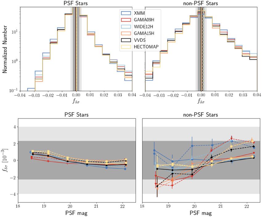
Publications of the Astronomical Society of Japan (2022), Vol. 74, No. 2                                                    423

high-resolution imaging that gives it a longer redshift base-      Lu et al. 2017); and (vii) other systematics from detector
line than the others. Hence the weak-lensing information           non-idealities—e.g., “tree rings,” “edge distortions” (Plazas
obtained from the HSC survey is complementary to those of          et al. 2014), and brighter-fatter effects (Antilogus et al.
the KiDS and DES surveys that probe weak-lensing effects           2014)—and from the atmosphere—e.g., differential chro-
at lower redshifts, but over a wider area than the current         matic refraction (DCR; Plazas & Bernstein 2012). There
HSC survey does. In addition, the excellent image quality          are other astrophysical uncertainties such as photometric
in HSC should enable us to pin down sources of systematic          redshift errors, intrinsic alignments of galaxy shapes, and
uncertainties in weak-lensing shear. In the coming decade,         the impact of baryonic effects (Mandelbaum 2018). In this
three ultimate imaging surveys will become available and           paper we focus on the observational effects in galaxy shape
promise to place further stringent constraints on cosmolog-        characterizations for weak-lensing measurements.
ical parameters including the nature of dark energy. Those             Because of the systematics mentioned above, it is neces-
are the Euclid satellite mission4 (Laureijs et al. 2011), Vera     sary to validate the shear catalog generation pipeline using
C. Rubin Observatory’s Legacy Survey of Space and Time5            image simulations. To develop simulations representative

                                                                                                                                   Downloaded from https://academic.oup.com/pasj/article/74/2/421/6547281 by guest on 29 June 2022
(LSST; Ivezić et al. 2019), and the Nancy Grace Roman             of the real data, the issue that arises here is how to rep-
Space Telescope6 (Spergel et al. 2015). Since the HSC data         resent the real observational conditions and the galaxy
is the deepest among the ongoing surveys, the HSC survey           properties in the HSC data maximally. Much effort has
can be considered as a precursor survey for LSST since they        been made to produce simulations that faithfully repre-
are both ground-based data and share similarities in the           sent the image characteristics that affect shear estimation
depth and image quality. Hence it is important and timely          (Mandelbaum et al. 2018a; Kannawadi et al. 2019;
to assess and figure out whether the quality and issues of the     MacCrann et al. 2022). Shear estimators must be calibrated
HSC data can meet requirements to use the weak-lensing             if the biases discovered with image simulations exceed the
measurements for cosmology, compared to the statistical            systematic error requirements of the weak-lensing survey.
errors of the current HSC data.                                    In addition, internal “null tests” related to galaxy and star
    However, weak-lensing shear is a tiny effect typically         shapes within the shear catalog are important to uncover
causing one percent ellipticities in the observed galaxy           the signatures of the aforementioned systematics (e.g.,
images, which are smaller than the root-mean-square (rms)          Mandelbaum et al. 2018b; Giblin et al. 2021; Gatti et al.
of intrinsic galaxy shapes. Thus the shear is only measurable      2021).
in a statistical sense. Hence an accurate weak-lensing mea-            In this paper, we describe the process to generate the
surement requires exquisite characterization of individual         three-year shear catalog for weak-lensing statistics from
galaxy images as well as control and calibrations of all           the HSC-SSP S19A internal data release (released in 2019
observational effects such as atmospheric effects (point-          September). First, we measure galaxy shapes using the re-
spread function and background noise) and the detector             Gaussianization method (reGauss; Hirata & Seljak 2003),
noise. It is important to ensure that residual systematic          and calibrate the shear estimation bias using HSC-like
errors are well below the statistical error floor so that any      galaxy image simulations following the formalism of Man-
physical constraints obtained from the weak-lensing mea-           delbaum et al. (2018a). We then calculate the requirements
surements are not biased. Observationally there are sev-           for cosmological analysis based on the survey parameters.
eral sources of systematic effects inherent in characterizing      We subsequently proceed with data quality control with
galaxy shapes, even in a statistical sense: (i) “noise bias”       “null tests” on the catalog following Mandelbaum et al.
due to the non-linear impact of noise on shear estimation          (2018b), which include tests related to PSF modelling, cross-
(Zhang & Komatsu 2011; Refregier et al. 2012); (ii) “model         correlations of galaxy shapes with random positions, star
bias” due to imperfect assumptions about galaxy mor-               positions and star shapes, and tests related to weak-lensing
phology (e.g., Bernstein 2010); (iii) “weight bias” caused by      mass maps.
shear-dependent weighting (e.g., Fenech Conti et al. 2017);            The structure of the paper is outlined as follows. In
(iv) “selection bias” originating from an improper treat-          section 2, we present the S19A internal HSC data release,
ment of selection effects around cuts (e.g., Mandelbaum            and outline the updates in the pipeline used to process the
et al. 2005); (v) systematics related to blending of galaxy        S19A data. In section 3, we calibrate reGauss galaxy shapes
light profiles (e.g., Li et al. 2018; Sheldon et al. 2020);        with realistic image simulations and characterize the three-
(vi) mis-estimation of the point-spread function (PSF; e.g.,       year HSC shear catalog. In section 4, we define the require-
                                                                   ments for the shape catalog on the PSF modelling and
4   https://sci.esa.int/web/euclid.                              shear inference to ensure that the three-year weak-lensing
5   https://www.lsst.org.                                        science is minimally affected by the systematics we listed
6   https://roman.gsfc.nasa.gov.                                 above. In section 5, we perform various systematic tests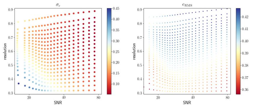
424                                                                           Publications of the Astronomical Society of Japan (2022), Vol. 74, No. 2

associated with the PSF modelling to ensure the quality of                               The PSFs on single exposures are modelled by PSFEx
PSF reconstruction and correction. Finally, we conduct null                           using a pixellated basis function, and in principle the over-
tests on the shear catalog in section 6, and summarize in                             sampled PSF model can be shifted by sub-pixel offsets using
section 7.                                                                            sinc interpolation. However, the Lanczos kernels, employed
                                                                                      by the original version of PSFEx in hscPipe v4 to approx-
                                                                                      imate the sinc kernel caused problems for images with the
2 HSC data and pipeline                                                               “very best seeing.” As shown in figure 9 of Aihara et al.
The HSC instrument (Furusawa et al. 2018; Miyazaki et al.                             (2019), the sizes of PSF models are less than the sizes of
2018a) is a wide-field optical imager mounted on the 8.2 m                            observed stars by 0.4% for regions with seeing FWHM
Subaru Telescope. The HSC-SSP (Aihara et al. 2018a) is                                (full width at half maximum) of around 0. 5.
a deep multi-band imaging survey with a target area of                                   For the second data release, as described in
1400 deg2 on the northern sky. The HSC pipeline (Bosch                                subsection 4.6 in Aihara et al. (2019), the pipeline resam-
et al. 2018) is a fork of Rubin’s LSST Science Pipelines                              pled the PSF models by interpreting the PSF models as

                                                                                                                                                         Downloaded from https://academic.oup.com/pasj/article/74/2/421/6547281 by guest on 29 June 2022
(Bosch et al. 2019); the fork is being developed to process                           a constant over each sub-pixel, rather than a continuous
the data from the HSC-SSP survey, while an updated version                            function sampled at the pixel center. This mitigated the
of Rubin’s LSST Science Pipelines will be used for LSST.                              PSF model errors for images with the “very best seeing,”
    The first public data release of HSC data (PDR1; Aihara                           reducing the fractional size residual between PSF models
et al. 2018b) was based on the S15B internal data release                             and observed stars from ∼ 0.4% to ∼ 0.1%. This new inter-
(released in 2016 January) and included images and cata-                              polation scheme is subsequently applied in the S19A image
logs processed with hscPipe v4 (Bosch et al. 2018).7 The                              processing.
first-year HSC shear catalog (Mandelbaum et al. 2018b)
was based on the S16A internal data release (released in
2016 August) and was also processed with hscPipe v4.                                  2.2 Improvements to the warping kernel
    The second public data release (PDR2) of images and cat-                          In the coaddition process, each single CCD image is con-
alogs was based on the S18A internal data release (released                           volved with a warping kernel to transform discrete (pixel-
in 2018 June) processed with hscPipe v6 (Aihara et al.                                lated) images into continuous images. The warped images
2019). There were major updates on the pipeline from                                  are subsequently resampled on to a common coordinate
hscPipe v4 to hscPipe v6 as summarized in Aihara et al.                               system.
(2019).                                                                                   For the data releases before S19A, a third-order Lanczos
    The shear catalog introduced in this paper is based on                            kernel was used to warp CCD images before coadding
the S19A internal data release (released in 2019 September)                           the images. As reported in subsection 6.4 of Aihara et al.
acquired from 2014 March to 2019 April. The S19A images                               (2019), the sizes of observed PSFs on coadds are 0.4% larger
are processed with hscPipe v7. Here we briefly summarize                              than that of reconstructed PSF models. Aihara et al. (2019)
the new features of hscPipe v7 updated from hscPipe v4                                showed that the amplitude of PSF size residuals decreases
that are important for weak-lensing measurements. In addi-                            when the order of the warping kernel is increased to the
tion, we summarize the changes in the observing strategy.                             fifth order.
As our first-year shear catalog helped to identify areas where                            A systematic bias on galaxy shape measurements stem-
progress was needed in the image processing pipeline, we                              ming from such a 0.4% fractional size residual in PSF size
expect this paper to provide a snapshot of the current state                          was not significant when compared to the first-year weak-
of the software pipeline, and to help in identifying further                          lensing science requirements (Mandelbaum et al. 2018b).
areas for progress.                                                                   However, for the three-year weak-lensing shear catalog,
                                                                                      the survey area has significantly increased and the science
                                                                                      requirements are consequently much tighter (see section 4).
2.1 Improvements in PSF modelling                                                     Therefore, we switch to using the fifth-order Lanczos
The HSC pipeline uses a repackaged version of PSFEx                                   warping kernel. The tests quantifying PSF model fidelity
(Bertin 2011) to estimate point-spread function (PSF)                                 are presented in section 5.
models on single exposures, and the PSF models on coadds
are estimated using the PSF models from each exposure,
while accounting for the warping kernel used for image                                2.3 Background subtraction
coaddition (Bosch et al. 2018).                                                       For the HSC first-year data release (DR1), the pipeline per-
                                                                                      formed a local background subtraction at the single expo-
7   See https://hsc-release.mtk.nao.ac.jp/doc/ for HSC-SSP data releases.           sure level with a 128 × 128 (∼22 × 22 ) pixel-mesh on
Publications of the Astronomical Society of Japan (2022), Vol. 74, No. 2                                                               425

each CCD individually. To estimate the sky background,
the pipeline averaged pixels in each pixel-mesh, ignoring
detected pixels. Then the background was modelled with
2D Chebyshev polynomials. After coadding single expo-
sures into coadds, the pipeline performed a background
subtraction with a larger (4k × 4k, or 11 × 11 ) pixel-mesh
(see Bosch et al. 2018 for more details) after masking out the
detections on coadds. This background-subtraction scheme
was found to cause over-subtraction around bright objects
since it subtracts flux from the wings of bright extended
objects along with the sky background (Bosch et al. 2018).
   In the second-year data release (DR2), the background-
subtraction scheme was updated as follows: at the single

                                                                                                                                               Downloaded from https://academic.oup.com/pasj/article/74/2/421/6547281 by guest on 29 June 2022
exposure level, the pipeline performed a global joint esti-
mation of the background using all the CCDs across the
                                                                   Fig. 1. 2D histogram of the i-band magnitude difference and the S19A
focal plane to reduce the aforementioned over-subtraction.         CModel magnitude. The magnitude difference (mag) is defined as the
In addition, the pipeline estimates and subtracts the “sky         S19A CModel minus the S16A CModel magnitude. Galaxies are matched
frame”—the mean response of the instrument to the sky              between S19A and S16A within the first-year HSC weak-lensing full-
                                                                   depth full-color region (Mandelbaum et al. 2018b) within 0. 5. The con-
for a particular filter. The sky frame is estimated from
                                                                   tours represent galaxy numbers of 102 and 105 , respectively. (Color
a clipped-mean of the pixel-mesh with detected objects             online)
masked out from many observations with large dithers
(see Aihara et al. 2019 for more details). The pipeline then       The details are summarized in the HSC third data release
applied the same background-subtraction scheme as before           paper (Aihara et al. 2022).
on coadds. This background-subtraction scheme preserves
the extended wings of bright objects; however, it influ-
ences the CModel measurement, which measures the flux              2.4 Bright star mask
by fitting the galaxy’s surface brightness profile with an         In this subsection we describe how bright star masks are
exponential and a de Vaucouleurs (de Vaucouleurs 1948)             applied to the weak-lensing shear catalog. Those who are
profile separately. The preserved wings of neighboring             interested in more details of the bright star mask construc-
bright objects and background residuals lead to larger esti-       tion, please refer to the PDR3 paper (Aihara et al. 2022).
mates of galaxy CModel radii and increase the CModel               The S19A bright star masks are created using the Gaia
flux estimates, especially for faint sources near bright           second data release (Gaia Collaboration 2018) as a ref-
objects.                                                           erence catalog in which Gaia magnitudes are converted
   With the intent to mitigate the under-subtraction               to HSC magnitudes. The star masks are defined for stars
problem and improve the performance of CModel measure-             brighter than 18th magnitude and for different types of arti-
ments, a local background subtraction with a 128 × 128             facts; halo, ghost, blooming, scratch, and dip. The scratch
(local) pixel-mesh is applied on coadds in S19A. In addition,      mask is designed to mask vertical stripes around bright stars
we use an improved global background-subtraction scheme            in long-wavelength bands (e.g., y band and NB1010 band)
during single-exposure image processing to remove global           due to the channel-stop, if the CCD is optically thin with
sky background and “sky frame” (see Aihara et al. 2022 for         respect to the wavelength (for more details, see Aihara et al.
more details). This background-subtraction scheme reduces          2022). Since the shear catalog is based on i-band images,
the aforementioned background residuals caused by the              the scratch mask is not considered for the shear catalog.
background-subtraction scheme in the second data release.          The dip mask is for masking over-subtracted regions in the
However, the CModel magnitude estimates in S19A are still          vicinity of a star due to the local background subtraction.
brighter than in S16A due to the influence of background           The over-subtraction affects the number count of source
residuals in S19A. As illustrated by the 2D histogram of the       galaxies but does not have significant influence on shape
i-band CModel magnitude difference between S19A and                estimation. In addition, applying the dip mask reduces the
S16A as a function of the S19A magnitude in figure 1, the          area significantly. Therefore, the dip mask is not consid-
histogram is skewed to negative mag. Figure 1 indicates           ered for the shear catalog. The shear estimation near stars
that objects appear brighter in S19A. In addition, we find         is tested in subsection 6.2.
that the galaxies with negative magnitude difference cluster           For the weak-lensing shear catalog, we adopt the star
around bright objects (e.g., bright stars and bright galaxies).    masks for halo, ghost, and blooming. The flags used for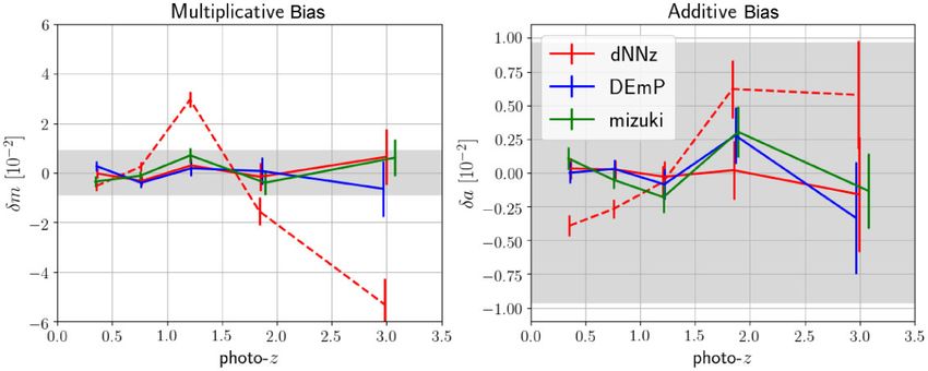
426                                                       Publications of the Astronomical Society of Japan (2022), Vol. 74, No. 2

Table 1. Flags of bright star masks considered in our shear       this requirement is imposed using the on-site quick-look
catalog. Objects flagged as True by any one of the masks are      software (Furusawa et al. 2018), which monitors the data
removed.                                                          quality with a lag of only a few minutes. Despite the fact
                                                                  that the requirement was relaxed, the mean i-band seeing
Mask flag                                             Meaning
                                                                  for the entire three-year data set used in this paper is
i mask brightstar ghost15                             Ghost       0. 59, similar to that of the first-year HSC shear catalog
i mask brightstar halo                                Halo        (Mandelbaum et al. 2018b). We look into the PSF model
i mask brightstar blooming                            Blooming
                                                                  errors in the regions observed with six dithers and with five
                                                                  dithers in section 5, the results of which do not show sig-
selection are summarized in table 1. The halo mask masks          nificant difference in the PSF model errors between the two
an extended smooth halo around a star, and the size of halo       observational strategies.
mask depends on the brightness of a star. To define the halo
mask, a median radial profile was computed for stars within

                                                                                                                                         Downloaded from https://academic.oup.com/pasj/article/74/2/421/6547281 by guest on 29 June 2022
a magnitude bin, and the mask was defined up to the scale         2.6 Full depth and full color cut
where the profile goes down to the background level. The          We restrict ourselves to regions that reach the approximate
size of halo mask decreases as a function of magnitude. The       full depth of the survey in all five broadband filters (grizy),
ghost mask is defined using the median radial profile and         in order to achieve better uniformity of the shear estimation
a cross-correlation with objects around bright stars where        and photometric redshift quality across the survey as was
ghost edges induce spurious detection of objects. The radius      also done in Mandelbaum et al. (2018b). This cut is imposed
of the ghost mask is 350 for stars brighter than the 7th        by requiring the average number of visits contributing to the
magnitude and 160 for stars between 7th and 9th magni-          coadds within HEALPix pixels (with NSIDE = 1024) to be
tude. The exact size and shape of the ghost depends on the        (g, r, i, z, y) ≥ (4, 4, 5, 5, 5).8 Note that this is different from
telescope boresight and a bright star, and fake objects out-      the requirement in the first-year shear catalog that was (g,
side the mask are found in some cases. To deal with such          r, i, z, y) ≥ (4, 4, 4, 6, 6). In the first-year shear catalog,
cases, we adopt a ghost mask with 50% larger than the             some of the i-band visits with the “very best seeing” were
standard size defined above. The blooming appears parallel        removed because of the inability to model the PSFs, and
to the channel-stop of a CCD, which is always horizontal in       thus the minimum number of i-band exposures was set to 4
the image because rotational dithers are not performed in         (Mandelbaum et al. 2018b). However, since the PSF deter-
the SSP survey. The scale of the blooming feature depends         mination in the HSC pipeline was improved as described
on the star brightness and positions on the CCD inputs,           in subsection 2.1, such exposures are added back to the
the maximum of which is ∼10 . To define the blooming             coadds. In addition, the 5-dithering strategy was adopted
mask, the cross-correlation measurement was performed             in November 2018. We thus set the requirement on the
along the horizontal and vertical directions, and a detec-        minimum numbers of average input visits for the i band to
tion excess along the horizontal direction was considered a       5. For the z and y bands, we set the requirement to 5 as
blooming. The blooming mask is defined as a function of           well, following the change in dithering strategy.
stellar magnitude.                                                    As will be discussed in subsection 5.2, we also remove
                                                                  a few regions with large average PSF size modelling errors.
                                                                  This PSF size modelling error cut reduces the survey area
2.5 Observing strategy                                            by ∼2.2%.
The observing strategy underwent a couple of changes in               After these cuts, the total area of the catalog is
order to increase the effective survey completion speed.          433.48 deg2 . The footprint of the galaxy catalog is divided
First, the number of dithers per pointing in the i, z, and        into six observational fields, i.e., XMM, GAMA09H,
y bands were reduced from 6 to 5 since 2018 November.             WIDE12H, GAMA15H, VVDS, HECTOMAP, the areas of
This change results in a survey depth that is shallower by        which are 33.17 deg2 , 98.85 deg2 , 121.32 deg2 , 40.87 deg2 ,
0.1 mag on average. The nominal 5σ depth for point sources        96.18 deg2 , and 43.09 deg2 . Figure 2 shows the i-band
in the i band was 26.2 for PDR2 based on S18A (see table 2        seeing map. Figure 3 shows the map of the number of i-
of Aihara et al. 2019). Our shear catalog only contains           band visits contributing to the coadd. Figure 4 shows the
galaxies with i-band magnitudes brighter than 24.5, and           seeing histograms, and figure 5 shows the noise variance
thus the change in depth is not expected to affect the statis-    histograms.
tical properties of the shear catalog significantly.
    The original requirement on the seeing conditions for
procuring i-band images was also relaxed from 0. 7 to 0. 9;   8   Each exposure of the CCD array is termed a visit.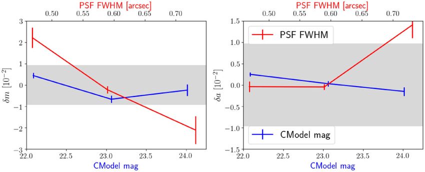
Publications of the Astronomical Society of Japan (2022), Vol. 74, No. 2                                                                        427

                                                                                                                                                        Downloaded from https://academic.oup.com/pasj/article/74/2/421/6547281 by guest on 29 June 2022
Fig. 2. Map of the i-band PSF FWHM across each field. The red dots are the sampling positions for PSFs and noise properties that will be used in
the HSC-like image simulation in subsection 3.2. The mean seeing over all of the fields is 0. 59. The circular region centered near (RA = 130.◦ 43,
Dec = −1.◦ 02) of the GAMA09H field is masked out due to the tracking error on the exposure visit 104934. (Color online)

3 Shear catalog                                                              from the coadded images. Every peak detected is identi-
                                                                             fied as a source and the connected nearby region above
In this section, we introduce the shear catalog measured
                                                                             the threshold is identified as the footprint of the source
from the HSC S19A i-band coadded images. We first
                                                                             detection.
review the shear estimation process in subsection 3.1. In
                                                                                 For the case that a footprint contains multiple sources,
subsection 3.2, we present the i-band image simulations
                                                                             these sources are taken as blended, and the HSC pipeline
used for the calibration of shear measurements. The selec-
                                                                             apportions the flux to these blended sources using the
tion criteria for the weak-lensing shear catalog are presented
                                                                             SDSS deblending algorithm (Lupton et al. 2001). This
in subsection 3.3. We subsequently determine the intrinsic
                                                                             deblending algorithm takes each peak as a “child” source
shape dispersion and the optimal weight for shear estima-
                                                                             of the “parent” detection. A template for each “child”
tion in subsection 3.4, calibrate the bias in the shear esti-
                                                                             is constructed with the assumption that each source has
mation in subsection 3.5, and quantify the amplitude of
                                                                             180◦ rotational symmetry around its detected peak. Then a
the calibration bias residuals in subsection 3.6. Selection
                                                                             scaling parameter is determined for each source by jointly
bias is estimated and calibrated in subsection 3.7. Finally,
                                                                             fitting the templates to the blended image.
the shear catalog is characterized in subsection 3.9 and our
                                                                                 After deblending, the HSC pipeline performs source
blinding strategy to avoid confirmation bias in weak-lensing
                                                                             measurement (e.g., flux, size, and shape) on each source.
analyses is presented in subsection 3.10.
                                                                             During the deblending and measurement of one detection,
                                                                             the pipeline replaces the footprints of other sources with
                                                                             uncorrelated Gaussian noise.
3.1 Shear estimation
3.1.1 Detection, deblending and source replacement                           3.1.2 Re-Gaussianization
In this sub-subsection, we briefly summarize the processes                   Galaxy shapes are estimated with the GalSim (Rowe et al.
of source detection, deblending, and source replacement                      2015) implementation of the re-Gaussianization (reGauss)
after coadding single exposures and background subtrac-                      PSF correction method (Hirata & Seljak 2003). This
tion based on hscPipe v7.                                                    moments-based method has been developed and used exten-
   The HSC pipeline (Bosch et al. 2018) performs a                           sively using data from the Sloan Digital Sky Survey (SDSS;
maximum-likelihood source detection with a 5σ threshold                      Mandelbaum et al. 2005, 2013). The outputs of the reGauss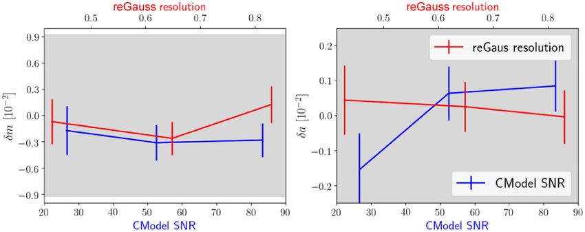
428                                                                  Publications of the Astronomical Society of Japan (2022), Vol. 74, No. 2

                                                                                                                                                             Downloaded from https://academic.oup.com/pasj/article/74/2/421/6547281 by guest on 29 June 2022
Fig. 3. Number of input visits contributing to the coadds in the i-band across each field. The mean number of input visits is 6.95 over all of the fields.
The way the visits are tiled across each survey area results in the repeated pattern of overlapping regions, with the number of inputs more than the
typical value (see Aihara et al. (2018a) for the tiling strategy). (Color online)

estimator are the two components of the ellipticity of each                    inverse variance weights to be used while performing the
galaxy:                                                                        ensemble average are the galaxy shape weights (w i ) defined
                                                                               as
               1 − (b/a)2
(e1 , e2 ) =              (cos 2φ, sin 2φ),                           (1)
               1 + (b/a)2
                                                                                             1
                                                                               wi =                  ,                                                (4)
where b/a is the axis ratio and φ is the position angle of                             σe;i
                                                                                        2
                                                                                            + erms;i
                                                                                               2

the major axis with respect to sky coordinates (with north
being +y and east being +x). Another important output of
the pipeline is the resolution factor R2 , which is defined for                where i is an index over galaxies, σ e is the per-component
each galaxy using the trace of the second moments of the                       1σ uncertainty of the shape estimation error due to photon
PSF (TPSF ) and those of the observed galaxy image (Tgal ):                    noise, and erms denotes the per-component rms of the galaxy
                                                                               intrinsic ellipticity. The parameters erms and σ e are modeled
               TPSF                                                            and estimated for each galaxy using image simulations, as
R2 = 1 −            .                                                 (2)
               Tgal                                                            will be discussed in subsection 3.4. The responsivity for the
                                                                               source galaxy population is estimated as
The resolution factor is used to quantify the extent to which
the galaxy is resolved compared to the PSF.

   For an isotropically-orientated galaxy ensemble dis-
                                                                                              i wi erms;i
                                                                                                    2

torted by a constant shear, the shear can be estimated with                    R=1−                      .                                           (5)
                                                                                                 i wi
a weighted average of the ellipticity of all galaxies:

         1                                                                     As the PSFs are nearly round, the responsivity for PSFs is
ĝα =      eα  ,                                                    (3)
        2R                                                                     approximately 1, and the shear distortion for a PSF image
where the shear responsivity (R) is the response of the                        is defined as gPSF,α = ePSF,α /2, where ePSF,α are the two com-
average galaxy ellipticity to a small shear distortion (Kaiser                 ponents (α = 1, 2) of PSF ellipticity defined with the second
et al. 1995; Bernstein & Jarvis 2002), and α = 1, 2 are                        moments of the PSF. We refer the reader to section 5 for
the indices for the two components of the ellipticity. The                     tests on PSF-related systematics.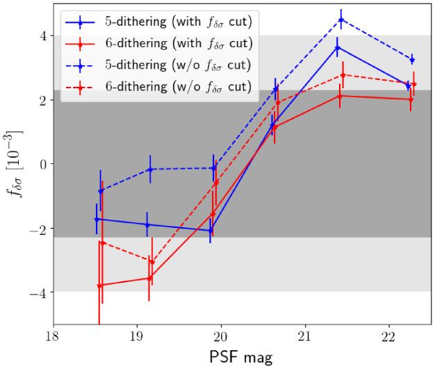
Publications of the Astronomical Society of Japan (2022), Vol. 74, No. 2                                                                           429

                                                                                                                                                           Downloaded from https://academic.oup.com/pasj/article/74/2/421/6547281 by guest on 29 June 2022
Fig. 4. The first six panels show the normalized number histograms of PSF FWHM for the galaxies in the HSC observational fields. The last panel
is the histogram for galaxies in all fields. The blue solid (red dashed) lines are for the HSC data (simulation). The blue (red) text and vertical lines
indicate the mean averages of the HSC data (simulation). The simulations are reweighted to mitigate the difference in the data due to the finite
sampling for each field. The gray lines show the histograms before the reweighting. (Color online)

3.1.3 Shear estimation bias                                                   can show slightly different biases for the two different shear
Since the reGauss algorithm is subject to certain forms of                    components (g1,2 ), we do not distinguish between the two
shear estimation bias (e.g., model bias, noise bias, and selec-               in this paper. In addition, the value of multiplicative bias is
tion bias), in this section, we define the calibration param-                 blinded in this paper to avoid confirmation bias in cosmo-
eters that will encapsulate those biases and review the cal-                  logical analyses.
ibrated form of the reGauss shear estimator. The relation                         We will estimate and model the multiplicative bias and
between the estimated shear and the true shear at the indi-                   the fractional additive bias for each galaxy as a function
vidual galaxy level is quantified by                                          of its properties (such as the signal-to-noise ratio SNR, R2 ,
                                                                              and galaxy redshift) in subsection 3.5.
ĝα;i = (1 + mi )gα;i + ai ePSF,α;i ,                                (6)          The multiplicative bias and the additive bias for the
                                                                              galaxy ensemble are the following:
where mi is the multiplicative bias and ai is the fractional
                                                                                       i wi mi
additive bias quantifying the fraction of the PSF anisotropy                  m̂ =              ,
                                                                                         i wi
(ellipticity) that leaks into the shear estimation. Terms
                                                                                       i wi ai ePSF,α;i
                                                                              ĉα =                        ,                                        (7)
involving spin-4 quantities, which average to zero when                                       i wi

averaging ĝα;i over all galaxies in the sample, are neglected.
                                                                              respectively. The calibrated shear estimator is defined as
The two components of the additive bias are thus given
by cα ≡ aePSF,α . Here we neglect the additive bias that is
                                                                                           i wi eα;i      ĉα
independent of PSF anisotropy since, using the image sim-                     ĝα =                  −        .                                    (8)
                                                                                      2R(1 + m̂) i wi   1 + m̂
ulation that will be introduced in subsection 3.2, we find
that the amplitude of that term is about 8 × 10⁻⁵ , which                         Note, here we neglect the selection bias due to the
is within the HSC three-year science requirements given in                    anisotropic selection of the galaxy ensemble. The shear esti-
section 4. We also conduct null tests that are sensitive to the               mation bias will be estimated using HSC-like image simu-
PSF-independent additive bias within the final shear catalog                  lations in subsection 3.5. The details of the simulation will
in subsection 6.1. Even though shear estimation algorithms                    be introduced in subsection 3.2.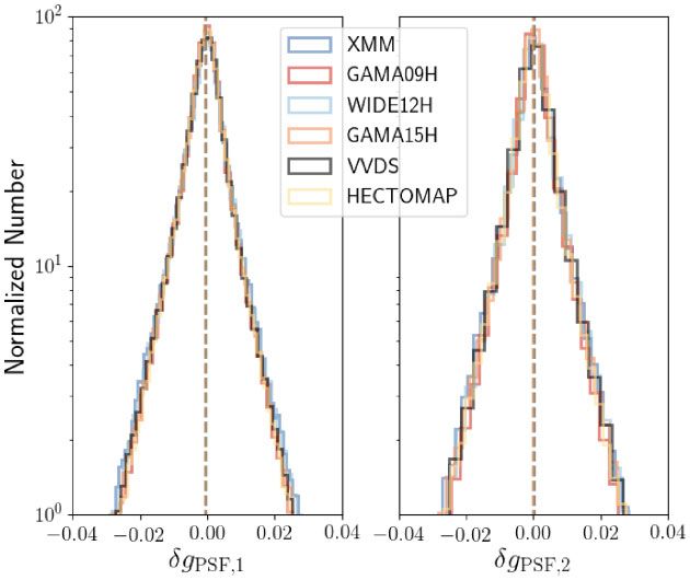
430                                                                Publications of the Astronomical Society of Japan (2022), Vol. 74, No. 2

                                                                                                                                              Downloaded from https://academic.oup.com/pasj/article/74/2/421/6547281 by guest on 29 June 2022
Fig. 5. Same as figure 4, but for noise variance. (Color online)

3.1.4 Selection bias                                                       divided into 2500 subfields and each subfield contains 104
Selection bias refers to a multiplicative or additive bias                 postage stamps, each of which is composed of 64 × 64
induced by a selection criterion that correlates with the                  pixels. The pixel scale is set to 0. 168 to match the pixel
true lensing shear and/or the PSF anisotropy. As a result of               scale of HSC.
the anisotropic selection, the selected galaxies that are suf-
ficiently close to the edge of the selection coherently align
in a direction that correlates with the lensing shear and/or               3.2.1 Input noise and PSF
the PSF anisotropy.                                                        The noise properties (including variance and spatial corre-
    Here we denote the multiplicative bias and the fractional              lations) and PSF models are the same in each subfield, while
additive bias caused by a selection as m̂sel and â sel , respec-          they vary between different subfields in the simulations. We
tively. They will be estimated for the galaxy ensemble using               sample 2500 noise variance values, noise correlation func-
the HSC-like image simulation in subsection 3.7. The final                 tions, and PSF models from a set of random positions on
shear estimator is                                                         the i-band coadded images on which the reGauss shapes
                                                                           are measured. The randomly sampled positions are shown
               ĝα − ĉαsel
ĝαfinal =                  ,                                       (9)    as red points in figure 2.
               1 + m̂sel
                                                                               Noise on the coadded images has a spatial correlation
where                                                                      between neighboring pixels, since the fifth-order Lanczos
                                                                          kernel used to warp CCD images during the coaddition
             âαsel    i wi ePSF,α;i
ĉαsel   =                                                        (10)    process (Bosch et al. 2018) results in correlated noise. We
                         i wi
                                                                           sample the noise correlations from the blank pixels (where
is the estimated additive selection bias.                                  no galaxy is detected) near the sampled random positions.
                                                                           Subsequently, the sampled noise correlations, which are
                                                                           noisy on the individual level, are randomly divided into
3.2 Image simulations                                                      eight groups, and stacked in each group to create eight dif-
In this subsection, we introduce the galaxy image simula-                  ferent well-measured noise correlation functions.
tions used to calibrate the galaxy shapes output by reGauss                    We first use the sampled noise variance of each subfield
on the HSC i-band coadded images. Our simulations are                      as the input noise variance for our preliminary simulations.
Publications of the Astronomical Society of Japan (2022), Vol. 74, No. 2 431
After populating galaxy images into each subfield, we mea- (2018a). In this paper, we use the training sample selected
sure the noise variance from blank (undetected) pixels on from the stack with the best seeing (0. 5) since it should
the preliminary simulations. The measured noise variances be the deepest sample among the three thanks to its best
are in general greater than the input noise variances due to seeing.
the light from neighboring detected sources and undetected Note, we do not inject parametric galaxies into images
sources underlying the blank pixels. We record the ratio as in, for example, MacCrann et al. (2022). Instead, we
between the measured noise variance and the input noise directly cut out postage stamps from the HST F814W
variance for each subfield, the average value of which is images. Since we do not perform any deblending or masking
1.25 across all subfields. Then we divide the sampled noise on the input HST images before shearing and transforming
variance by this ratio for each subfield, and the rescaled vari- the noise property, all of the neighboring sources are kept
ances are used as the inputs of our fiducial simulations. By on the postage stamp to reproduce the effects of both rec-
rescaling the sampled noise variances, we match the noise ognized and un-recognized blends. We do not input star
variances measured from the simulations to those measured images into the simulation. Stars could appear on galaxy
Downloaded from https://academic.oup.com/pasj/article/74/2/421/6547281 by guest on 29 June 2022
from the HSC data in a consistent manner. In contrast, we outskirts (not at the centers of the postage stamp) if they
did not perform such a rescaling in the first-year HSC-like happens to reside in close proximity to the simulated central
image simulations (Mandelbaum et al. 2018a), but rather galaxy. We will further test the influence of stellar contam-
inconsistently matched the input noise variances in the sim- ination in our shear catalog in sub-subsection 3.3.1.
ulation to the measured noise variances in the S16A HSC GalSim (Rowe et al. 2015), which is an open-source
data, which results in a larger noise variance in image sim- package for galaxy image simulations, is used to simulate
ulations compared to reality. HSC-like images using the COSMOS HST images in our
To mitigate the differences between the simulations simulations. The original HST PSF is deconvolved from
and the HSC data due to the finite sampling of noise each input HST postage stamp and then the image is rotated
and PSF, we reweight each subfield in the simulations by a random angle, sheared by a known input shear distor-
such that the seeing and noise variance histograms closely tion, convolved with a collected HSC PSF model, sampled
match the real data. Note that we do not reweight the at the HSC pixel scale, and downgraded to an HSC noise
simulations according to any properties of the input level. The noises and PSFs used in the simulations are those
galaxies. The reweighting is conducted separately for each introduced in sub-subsection 3.2.1.
HSC observational field. The seeing (PSF FWHM) his- Each subfield is designed specifically to include 90◦
tograms and noise variance histograms for the observa- rotated (intrinsically orthogonal) pairs of galaxies that can
tions and the simulations are shown in figures 4 and 5, be used to nearly cancel out shape noise (Massey et al.
respectively. 2007b). By keeping track of the members of each orthog-
Note that the input PSF models do not include PSF model onal pair, the analysis framework provides options to
errors; that is, the PSF is assumed to be known perfectly. apply this cancellation or not. The orthogonal pairs will
In addition, we assume the sky subtraction is perfect, and also be used to derive shape measurement error, weight
the residuals of the sky background are not included in the bias, and selection bias in the shear estimation following
simulations. As these observational conditions are obtained Mandelbaum et al. (2018a).
from coadded images, the systematics related to the coad-
dition process can not be tested with the simulations.
3.3 Weak lensing galaxy sample
3.2.2 Input galaxy 3.3.1 Galaxy selection
Mandelbaum et al. (2018a) selected galaxy training sam- We run hscPipe v7, the pipeline used to process the
ples with CModel magnitudes less than 25.2 from the HSC S19A internal data release along with the same configu-
Wide-depth catalogs detected from three stacks of the HSC ration options, on the simulations for source detection and
Deep/Ultradeep images with typical seeings of 0. 5, 0. 7, and deblending. Subsequently, hscPipe v7 is used to perform
1. 0, respectively, in the COSMOS region (Aihara et al. magnitude, size and shape measurements on the deblended
2018b). Mandelbaum et al. (2018a) determined the cen- sources. For all of the analyses shown in this paper based
troids of these galaxies on the exposures of the COSMOS on our image simulations, a basic set of flag cuts, listed in
HST Advanced Camera for Surveys (ACS) field (Koekemoer the “Basic flag cuts” section of table 2, are imposed. Since
et al. 2007) in the F814W band. Square postage stamps cen- our simulations do not include image artifacts, only the fol-
tered at the galaxy centroids with width = 10. 752 (64 HSC lowing flags actually influence the source selection in the
pixels) were cut out from the HST exposures. The details simulations: i detect isprimary, i sdsscentroid flag,
of the training samples are described in Mandelbaum et al. and i extendedness value.432 Publications of the Astronomical Society of Japan (2022), Vol. 74, No. 2
Table 2. Weak lensing cuts.∗
Cut Meaning
— Basic flag cuts —
i detect isprimary == True Identify unique detections only
i deblend skipped == False Deblender skipped this group of objects
i sdsscentroid flag == False Centroid measurement failed
i pixelflags interpolatedcenter == False A pixel flagged as interpolated is close to object center
i pixelflags saturatedcenter == False A pixel flagged as saturated is close to object center
i pixelflags crcenter== False A pixel flagged as a cosmic ray hit is close to object center
i pixelflags bad== False A pixel flagged as otherwise bad is close to object center
i pixelflags suspectcenter == False A pixel flagged as near saturation is close to object center
i pixelflags clipped == False Source footprint includes clipped pixels
i pixelflags edge == False Object too close to image boundary for reliable measurements
Downloaded from https://academic.oup.com/pasj/article/74/2/421/6547281 by guest on 29 June 2022
i hsmshaperegauss flag == False Error code returned by shape measurement code
i hsmshaperegauss sigma ! = NaN Shape measurement uncertainty should not be NaN
i extendedness value ! = 0 Extended object
— Galaxy property cuts —
i cmodel flux/i cmodel fluxerr≥10 Galaxy has high enough S/N in i-band
i hsmshaperegauss resolution ≥0.3 Galaxy is sufficiently resolved
(i hsmshaperegauss e12 +i hsmshaperegauss e22 )1/2 < 2 Cut on the amplitude of galaxy ellipticity
0 ≤i hsmshaperegauss sigma ≤0.4 Estimated shape measurement error is reasonable
i cmodel mag − a i ≤24.5 CModel Magnitude cut
i apertureflux 10 mag ≤25.5 Aperture (1 diameter) magnitude cut
i blendedness absPublications of the Astronomical Society of Japan (2022), Vol. 74, No. 2 433
have multi-band image simulations. This multi-band detec-
tion cut removes a very small fraction (< 1%) of galaxies
that pass other selection thresholds. Therefore, the multi-
band cut is not likely to cause significant selection bias on
the shear estimation. On the other hand, this multi-band
cut helps remove junk detections and artefacts (Hildebrandt
et al. 2017).
Compared with the S16A data, the S19A data is pro-
cessed with a global background-subtraction scheme as
summarized in subsection 2.3. The under-subtraction of sky
background in this scheme increases the CModel flux esti-
mation near bright objects, which makes cuts on CModel
flux inefficient at removing the galaxies beyond the HST
Downloaded from https://academic.oup.com/pasj/article/74/2/421/6547281 by guest on 29 June 2022
magnitude limit and the fake detections caused by back-
ground light residuals in the observations. We find a mis-
Fig. 6. Stellar contamination fraction due to the incorrect classification
match in the SNR–R2 2D histograms between the S19A
by hscPipe v7, estimated after application of the weak-lensing cuts in HSC data and the simulations at the faint end when simply
table 2. We show the stellar contamination fraction as a function of using the first-year i-band cuts summarized in table 4 of
i-band CModel magnitude for three different seeing conditions (i.e.,
Mandelbaum et al. (2018b). There are more extended faint
BEST, MEDIAN, and WORST) estimated with reference to COSMOS HST
star–galaxy classifications used as an estimate of ground truth. Error detections that are very likely to be fake detections in the
bars show the Poisson uncertainties. Dashed lines show the stellar con- HSC data than in the simulations. Therefore, we apply an
tamination fractions for all magnitude bins in the corresponding seeing additional cut on i-band 1 -diameter-aperture magnitudes
samples. (Color online)
(magA ) at 25.5 to remove the fake detections that cannot
be reproduced in the simulations. The additional aperture
seeing values of 0. 5, 0. 7, and 1. 0, respectively (Aihara et al. magnitude cut removes 3.9% of the galaxies that pass other
2018b). Even in the worst seeing conditions, the stellar selection cuts. The selection bias due to the cuts is quantified
contamination fraction is below 0.2% for galaxies with in subsection 3.7.
i-band magnitudes brighter than 22, increasing to 0.5% at To study the influence of the selection function of
the faintest end of the shear catalog with i-band magnitude hscPipe v7 source detection on our galaxy sample, in cases
close to 24.5. Hence we conclude that the shear estima- where no object is detected within 5 pixels from the center
tion biases from the misclassification of stars as galaxies is of a simulated postage stamp, we artificially force one detec-
negligible, since the fraction of misclassified stars is less than tion with its peak at the center of the stamp. Flux, size, and
0.5%. shape measurements are conducted on the artificially forced
We do not apply any cuts to remove the potential con- detections. We find that the number of these forced detec-
tamination from binary stars as in Hildebrandt et al. (2017). tions that enter the weak-lensing sample after the weak-
Even though we do find that objects in the weak-lensing lensing cuts are applied is far less than 0.1% of the total
sample with extremely large ellipticity |e| > 0.8 and i-band galaxy number in the weak-lensing sample, which indicates
determinant radius rdet < 10−0.1r+1.8 arcsec show a charac- that the selection function of the source detector has a neg-
teristic stellar locus in the (g − r, r − i) color–color his- ligible influence on the weak-lensing sample; therefore, the
togram, its number fraction is only ∼ 0.46% of the weak- selection bias from the source detector is negligible. This
lensing galaxy sample, which is not likely to cause biases is aligned with our expectations, since the 5σ detection
beyond the weak-lensing requirements. We will remove limit for point sources is 26.2 mag in the i band, and our
these potential binary stars from our sample in the three- weak-lensing galaxy sample is selected with an i-band mag-
year cosmological analysis. nitude cut at 24.5, far brighter than the detection limit.
In addition to the i-band cuts, we follow Mandelbaum We note that one limitation of our simulations is that sev-
et al. (2018b) and apply a multi-band detection cut to ensure eral defects from real data (e.g., sky background residuals,
that we have enough color information to compute photo- optical ghosts, very bright stars, etc.) that can affect the
metric redshifts. The multi-band color cut requires at least object detection are not included.
two other bands (out of grzy bands) to have at least a 5σ
CModel detection significance (i.e., SNR > 5). The multi- 3.3.2 Galaxy properties
band detection cut is applied only on the HSC data but not The 1D normalized number histograms for i-band galaxy
on the image simulations since, unfortunately, we do not properties (i.e., CModel SNR, reGauss resolution, CModel434 Publications of the Astronomical Society of Japan (2022), Vol. 74, No. 2
Downloaded from https://academic.oup.com/pasj/article/74/2/421/6547281 by guest on 29 June 2022
Fig. 7. Normalized number histograms of i-band properties including CModel SNR (upper left), reGauss resolution (upper right), CModel magnitude
(lower left), and reGauss ellipticity magnitude (lower right), for galaxies in all fields combined. The blue solid (red dashed) lines are for the HSC data
(simulation). The blue (red) text and vertical lines indicate the mean averages of the HSC data (simulation). (Color online)
magnitude,
reGauss ellipticity magnitude defined as presented in this paper. The match in SNR distribution
|e| = e1 + e22 ) in the HSC observations and the simula-
2 improves because we rescale the sampled noise variance for
tions are shown in figure 7. When plotting the histograms, a consistent match between the measured noise variances
we adopt the same upper limit on the i-band CModel SNR from the HSC data and those from the simulations as dis-
(SNR < 80) as Mandelbaum et al. (2018a) to compare our cussed in sub-subsection 3.2.1. Furthermore, the matches
results with those shown in the HSC first-year image sim- between the 2D histograms are visually better than those
ulation paper. We do not find significant differences in the of the first-year HSC simulations shown in figure 9 of
shapes of the number histograms between the HSC data and Mandelbaum et al. (2018a), primarily due to the improve-
the simulations. The relative difference of the mean values ment in the match between the SNR histograms.
averaged across all of the fields for these properties between In addition, compared to the state-of-art image sim-
the data and the simulations are 0.5% (CModel SNR), ulations in other weak-lensing surveys, e.g., figure 3 in
0.2% (reGauss resolution) 0.1% (CModel mag), and 0.8% MacCrann et al. (2022) from the DES survey and figure 9
(|e|), all of which are less than 1%. Finally, we show the 2D in Kannawadi et al. (2019) from the KiDS survey, our sim-
joint histograms of these galaxy properties in figure 8. ulations generally have better matches to the observations
Compared to the first-year HSC-like image simulations in the histograms of galaxy brightness, size, and shape.
(see Mandelbaum et al. 2018a, figure 8), the three-year
HSC-like simulations have a better match to the HSC data
in the SNR histogram. The average SNR over all fields 3.4 Optimal weighting
was relatively less than the observed SNR by ∼5% in In this subsection, we estimate and model the statistical
Mandelbaum et al. (2018a), while the discrepancy decreases uncertainties from photon noise (shape measurement error)
to ∼ 0.5% for the three-year HSC-like image simulations and shape noise (intrinsic shape dispersion) as functions ofPublications of the Astronomical Society of Japan (2022), Vol. 74, No. 2 435
Fig. 8. Color maps of the 2D histograms for the HSC data. The panels from left to right show the (SNR, R2 ), (SNR, |e|), and (SNR, CModel magnitude)
Downloaded from https://academic.oup.com/pasj/article/74/2/421/6547281 by guest on 29 June 2022
histograms, respectively. The solid (dashed) lines show the contours for the HSC data (simulation). The contours in panels from left to right are
defined at (0.90, 0.60, 0.30, 0.12), (0.76, 0.54, 0.26, 0.14), and (0.68, 0.34, 0.14) of the maximums of the corresponding histograms. (Color online)
Weight
Resolution
Resolution
Resolution
Fig. 9. Left: 1σ per-component shape measurement uncertainty (σ e ) estimated with the simulations in different (SNR, R2 ) bins. Middle: Estimated
per-component intrinsic shape dispersion (erms ) following equation (12). Right: Estimated optimal weight.
galaxy properties, and determine the optimal weight for the interpolation of this ratio. As shown, the shape measure-
shear estimation. ment error from photon noise is a decreasing function in
We first use the simulations to estimate the 1σ per- the SNR direction and the R2 direction since noise has less
component shape uncertainty due to photon noise (σ e ) influence on bright, large galaxies.
and model it as a function of galaxy properties (i.e., SNR Using galaxies in the real HSC shear catalog, we estimate
and R2 ) following the formalism given in Appendix A of the per-component intrinsic shape dispersion (erms ) by sub-
Mandelbaum et al. (2018a). In the estimation, we use the tracting off (in quadrature) the shape measurement error
orthogonal galaxy pairs to nearly cancel out shape noise from the shape dispersion such that
and measure the statistical error due to photon noise.
i e1;i + e2;i − 2σe (SNRi , R2;i )
2 2 2
We define a sliding window in the (SNR, R2 ) plane with
erms = , (12)
an equal-number binning scheme and estimate σ e in each 2Ngal
bin. The results of this process are shown in the left-hand
panel of figure 9. In order to estimate σ e for each galaxy in where i is the galaxy index and Ngal refers to the number of
the catalog, we fit a power-law σ e (SNR, R2 ) to the estimated galaxies in the galaxy ensemble. This estimate is computed
σ e , such that in each sliding window, and the estimated intrinsic shape
dispersion as a function of the position in the (SNR, R2 )
−0.942 −0.954
SNR R2 plane is shown in the middle panel of figure 9. As shown, the
σe = 0.268 , (11)
20 0.5 intrinsic shape is a relatively flat function on the 2D plane,
with a value of around 0.4 for most of parameter space.
and linearly interpolate the ratio of the estimated values to The corresponding optimal weight defined in equation (4)
the fitted power-law based on the log10 (SNR) and R2 values. is shown in the right-hand panel of figure 9. The shape dis-
For SNR and R2 outside the bounds of the sliding window, persion is relatively flat with a value around 0.4; therefore,
the nearest point within the sliding window is used for the we linearly interpolate the function in the 2D plane to modelYou can also read