The Perceptual Primacy of Beauty: Deep net features learned for computer vision linearly predict image aesthetics, arousal & valence - but ...

The Perceptual Primacy of Beauty: Deep net features
  learned for computer vision linearly predict image
aesthetics, arousal & valence – but aesthetics above all

                                              Abstract

         How well can we predict human affective responses to an image from the purely
         perceptual response of a machine trained only on canonical computer vision tasks?
         We address this question with a large-scale survey of deep neural networks de-
         ployed to predict aesthetic judgment, arousal, and valence for images from multiple
         categories (objects, faces, landscapes, artwork) across two distinct datasets. Im-
         portantly, we use the features of these models without any additional learning. We
         find these features sufficient to predict average ratings of aesthetics, arousal, and
         valence with remarkably high accuracy across the board – in many cases beyond
         the ratings presaged by even the most representative human subjects. Across our
         benchmarked models, which include Imagenet-trained and randomly-initialized
         convolutional and transformer architectures, as well as the encoders of the Taskon-
         omy project, a few further trends become evident. One, predictive power is not a
         given: Randomly-initialized models categorically fail to predict the same quantities
         of variance as trained models. Two, object and scene classification training produce
         the best overall features for prediction. Three, aesthetic judgments are the most
         predictable of the affective responses, superseding arousal and valence. This last
         trend, especially, highlights the possibility that aesthetic judgment may be a form
         of ‘elemental affect’ embedded in the perceptual apparatus – and directly available
         from the statistics of natural images. The contribution of such a mechanism could
         help explain why our otherwise affectless machines predict affect so accurately.

1   Disclaimer
This manuscript is a work in progress, and has not yet undergone peer review. Some content
may be subject to change, and some citations may be missing or erroneous. Please email con-
well[at]g[dot]harvard[dot]edu for clarifications or comments.

2   Introduction
Without significant hyperbole, the decade spanning 2011 to 2021 could be called the decade of
the perceptual machine. Detection, segmentation, localization, recognition – perceptual tasks once
thought the exclusive purview of biological systems – are now well within the capabilities of modern
machine learning algorithms [1]. In addition to their raw competence, these machines now serve as
some of the most predictive models to date of the biological systems they imitate [2].
The power of these machines as empirical tools lies not in their performance on any given task per se,
but in the constraints under which they perform those tasks – constraints that allow us, as researchers,
to more closely triangulate the kinds of computational (information processing and representational)
competencies that might undergird the performance of those tasks in nature.

After all, there are certain things these perceptual systems generally are, and certain things they
definitively are not. What they generally tend to be are highly trained specialist deep neural networks
designed to transform various digital inputs (pixels, waveforms) into one of several (usually well-
defined) outputs. The transformations in this case tend to be serial, mostly feedforward, deterministic
(that is, not stochastic), and most importantly differentiable. What they tend not to be generalists [3].
Trained for only one task, they tend usually to be able to perform only that task, and must undergo
significant retraining or reformatting to perform other tasks to par – often catastrophically forgetting
the representations necessary for the first task if they do.
Most importantly for the purposes of the present analysis, perceptual machines are in no way affective,
with states that correspond under any definition to biological emotion. With these constraints in
mind, the central questions we ask here are twofold: One, can the responses of our purely perceptual,
affectless machines – never remotely trained on affect – nonetheless predict human affect from a
given stimulus to a reasonable extent? And if they can, how might that inform our conceptualization
of affect more broadly? Of particular interest to us here is beauty, the perceptual mereology of which
remains a matter of sometimes hotly contested debate [4–11].
Previous work has addressed questions like the ones we’ve posed here in multiple ways, but has
typically done so by retraining to some degree a perceptual machine specifically for the task of detect-
ing emotion or predicting aesthetic value. Kragel et al. [12] propose EmoNet: a deep convolutional
network architecture refitted to ’output ... a probabilistic representation of the emotion category of a
picture or video’. Iigaya et al. [13] retrain the final 3 layers of a standard VGG16 architecture on
’averaged liking ratings’.
In this work, our intent is to assess whether or not we can predict affect directly from the feature
spaces of a perceptual machine without any further modification, retraining or reshaping – which is
to say, whether or not information about affect is already inherent to the learned representations of
neural networks never trained on affect, and trained only on the various canonical computer vision
tasks that define the current state of the field. To this end, we use over 90 distinct neural network
models, ratings of aesthetics, arousal and valence from over 700 subjects, and two distinct image
sets – ensuring any conclusions we draw are not the product of mere statistical flukes, but of robust,
identifiable trends across large amounts of data. If we are to take the implications of predicting affect
from the computational competences of perception seriously, we must first assure those predictions
are sound.

3     Methods
3.1   Image Datasets
As our primary dataset, we use OASIS [14], a set of 900 images spanning 4 distinct categories
(people, animals, objects and scenes), with normative ratings of arousal and valence from 822 human
subjects. Ratings of beauty (from another 751 human subjects) we obtain from a separate source
[15]. We complement OASIS with a secondary dataset consisting of 512 images across 5 distinct
categories (art, faces, landscapes, internal & external architecture), but for which only ratings of
beauty are available. This secondary dataset not only allows us to explore various questions OASIS
does not (judgments of art versus judgments of natural scenes), but to internally replicate at least a
subset of the results we obtain with OASIS.
As a first step to processing these datasets, we calculate two forms of reliability as gauges for the
comparative performance of our models. The first – what we call leave-one-out reliability – involves
iteratively removing one subject from the subject pool and correlating that subject’s average with the
average of the subjects remaining. The 95% confidence interval over these leave-one-out correlations
for all subjects gives us a sense of how well on average a randomly selected human subject is able to
predict the mean rating for a given set of stimuli. Our second reliability metric – the splithalf reliability
– involves splitting the group-level data in half 10000 times and correlating each half with the other.
The 95% confidence interval over these splithalves (corrected with the Spearman-Brown prophesy
formula) provides a more concrete upper bound (a noise ceiling) on how well any predictive model
could do in predicting the mean rating for a given set of stimuli. We use both of these thresholds as a
point of reference for the performance of our models.

                                                     2

3.2   Candidate Models
In total, we survey a set of 95 distinct models (165 including the randomly-initialized versions of
each). These models are sourced from three different repositories: the Torchvision (PyTorch) model
zoo [16], the pytorch-image-models (timm) library [17], and the Taskonomy (visualpriors) project
[18–20]. The first two of these repositories offer pretrained versions of a large number of object
recognition models with varying kinds of architectures: convolutional networks, vision transformers,
normalization-free networks and MLP-Mixer models. Note, however, that all of these models are
feedforward. For each of these ’ImageNet’ models, we extract the features from one trained and
one randomly initialized variant (using whatever initialization scheme the model authors deemed
best) so as to better disentangle what training on object recognition affords us in terms of predictive
power. The Taskonomy models consist of a core encoder-decoder architecture trained on 24 different
common computer vision tasks, ranging from autoencoding to edge detection. The models are
engineered in such a way that only the architecture of the decoder varies across task, allowing us to
assess (after detaching the encoder) what effect different kinds of training has on predictive power,
independent of model design.

3.3   Feature Regression
To predict ratings of beauty, arousal and valence for each of the images in our datasets from a given
set of deep net features, we use regularized linear regression with cross-validation. The process of
prediction progresses in multiple phases. The first phase (extraction) involves passing each image in
a dataset through each layer in a given deep net, cataloguing all features generated at each successive
stage of computation. The second phase (regression) iteratively takes the features from a single layer
and employs them as regressors in a linear model where the regressand is the rating (arousal, valence
or beauty) for a given image. The use of regularized (ridge) regression allows us to take advantage of
a cross-validation procedure called generalized cross-validation (a hyperefficient, linear algebraic
form of leave-one-out cross-validation) [21]. This brings us to third phase (cross-validation and
scoring). Because the dimensionality of deep net feature spaces varies widely (from the order of 103
to 107 ), we use generalized cross-validation first to choose a reasonable lambda parameter for a given
feature space from a sample of 25 values evenly spaced on a log scale from -1 to 5, minimizing an
explained variance score. We then correlate the leave-one-out cross-validated predicted ratings from
the optimal lambda regression for a given set of images with the actual ratings to produce an overall
score for the feature space in question. We repeat this process until we have a score (Pearson’s r)
per model layer per model per affect category per image category per dataset. (A slightly modified
version of this analysis, in which we decouple hyperparameter selection from prediction with a
candidate model we subsequently remove from the analysis, is shown in the Appendix). All phases
in this process are programmed with Python’s Scikit-Learn package [22].

4     Results
Unless otherwise noted, we use the following convention in the reporting of means: arithmetic mean
[lower 95% bootstrapped confidence interval, upper 95% bootstrapped confidence interval].

4.1   Object recognition models often predict group-level affect ratings as well as the most
      representative human subjects, and decently close to the overall noise ceiling.
Though their scores do vary by image category (see Section 4.6), object recognition (ImageNet-
trained) models perform well in the prediction of group-level affect ratings across all 3 types of affect
(beauty, arousal and valence) and across both datasets surveyed. When considering the full OASIS
dataset (without subdivision into image category), mean scores are: 0.717 [0.708, 0.726] for arousal;
0.693 [0.682, 0.705] for valence; and 0.769 [0.760, 0.778] for beauty. When considering the full
Vessel dataset (which measures beauty alone), mean scores are 0.696 [0.689, 0.702].
To better gauge these scores in context, we can compare them to our estimates of reliability. In the
OASIS dataset, mean leave-one-out reliabilities are: 0.481 [0.458, 0.504] for arousal, 0.643 [0.632,
0.654] for arousal; 0.752 [0.739, 0.765] for valence; and 0.643 [0.632, 0.654] for beauty. In the
Vessel dataset (beauty only), mean leave-one-out reliability is 0.461 [0.408, 0.513]. What this means
is that apart from valence, ImageNet-trained models are on average substantially more predictive of
group-level affect ratings than a typical held-out subject. We can quantify the comparison to human
subjects even more precisely by iteratively subselecting out the subjects with the lowest correlations

                                                   3

to the group mean from subject pool, desisting when the mean of the leave-one-out correlations is
minimally different from the mean score of the models. This allows us to report the percentage of
subjects whose predictive power (representativeness) of the group-level rating is less than that of the
average model: 85% for arousal, 21% for valence, and 83% for beauty in the OASIS dataset. In the
Vessel dataset (beauty only), no single human subject is as predictive as the average model.
While leave-one-out reliability provides a sense of how well an individual subject’s ratings can
predict the group-level averages, the splithalf reliability provides a sense of how well the ratings
data more generally can predict itself – and thus delimits a noise ceiling on how well we might
expect any predictive model to do in predicting the group averages given inconsistency in response
across participants. In the OASIS dataset, the splithalf reliabilities (across 10000 splits, Spearman-
Brown corrected) are: 0.963 [0.945, 0.975] for arousal; 0.992 [0.990, 0.994] for valence; and 0.989
[0.984, 0.992] for beauty. In the Vessel dataset (beauty only), the splithalf reliability is 0.862 [0.814,
0.897]. By squaring the mean splithalf reliability, dividing that value by the score for each model,
then averaging the resultant proportion across models, we can derive a measure of mean variance
explained. In the OASIS dataset, the mean variance explained is: 0.555 [0.542, 0.569] for arousal,
0.491 [0.475, 0.507] for valence, 0.606 [0.592, 0.62] for beauty. In the Vessel dataset (beauty only),
the mean variance explained is 0.652 [0.639, 0.664].
Taken together, these results – in which many of our predictions exceed the predictions of even the
most representative human subjects and the mean variance explained is well over 50% for all 4 of
our affect ratings – suggest our perceptual models, never trained on affect, have nonetheless learned
statistical proxies of affect sufficient to predict with nontrivial accuracy the kinds of responses an
average human subject will have in response to an image. A summary of scores across model and
model layer relative to our two reliability thresholds is available in Figure 1; a summary of the more
detailed comparison to human subjects is shown in Figure 2.

4.2   Aesthetics is the most predictable of the affective measures.
While the features of our object recognition models do attain relatively high predictive accuracy for all
3 affect ratings, the overall highest accuracies we obtain are in predictions of beauty. We can quantify
this advantage across the multiple modalities we use to convey or contexualize performance in Section
4.1 above. First and foremost is sheer difference in scores: pairwise t-tests (Holm-corrected) between
the three kinds of affect rating (only available in the OASIS dataset), reveal significant differences in
beauty versus arousal (t(138) = 8.21, p = 4.15− 13, Hedge’s g = 1.39) and beauty versus valence
(t(138) = 10.33, p = 42.06− 18, Hedge’s g = 1.75). Transforming our scores into the proportion of
(explainable) variance explained, so as to account for differences in the overall noise ceiling (and by
association how differentially well our models could theoretically perform in predicting each affect
rating) we can compute the same pairwise t-tests again, showing the same significant differences in
beauty versus arousal (t(138) = 5.22, p = 6.43− 7, Hedge’s g = 0.82) and beauty versus valence
(t(138) = 10.8, p = 1.32− 19, Hedge’s g = 1.83).
Even controlling for differences in inter-rater reliability, then, aesthetics dominates as the most
predictable of the affective measures. So robust is this advantage that it recapitulates across almost all
of the distinct image subcategories in the OASIS dataset, as evidenced by pairwise comparisons that
expand from testing difference in affect category alone to the interaction of affect category and image
category. There are significant differences (p < 0.001, Holm-corrected; mean Hedge’s g = 1.89) in
beauty versus arousal and versus valence in all image categorys except for Object, where only the
difference in beauty versus arousal is significant.
The differences between beauty, valence and arousal are particularly intriguing given the (Pearson)
correlations between them: beauty with valence yields r = 0.75; beauty with arousal yields r =
0.160; arousal with valence yields r = −0.058.

4.3   Trained models are categorically more predictive of affect than untrained models.
Given the size, complexity and sometimes rich structure of feature spaces inherent to deep neural
networks, there have been a number of cases in recent years in which randomly initialized networks
– never trained – have demonstrated predictive power as robust as that of fully trained networks.
While not entirely unanticipated given certain architectural priors (e.g. translational invariance in
convolutional neural networks), this can sometimes lead to the impression that neural networks are
little more than highly generalizable random number generators, on which training has little impact.

                                                    4

Here, we show to the contrary that training matters. For every ImageNet-trained model (tested on
every affect rating and image category), we compare that model’s max score with the max score of its
randomly-initialized counterpart. To test significance, we perform pairwise t-tests across each image
category, affect rating and dataset, with Holm corrections for multiple comparisons. We find all
pairwise differences are significant (at p < 0.001) and with often massive effect sizes (mean Hedge’s
g = 7.99). Not a single randomly initialized model outperforms its ImageNet-trained counterpart.

4.4       Representations learned for object and scene recognition are the overall best
          representations for predicting affect.
The results we have reported so far have been exclusive to models trained on object recognition
through the ImageNet challenge. But how does object recognition fare in relation to other tasks
in terms of providing features relevant for the prediction of affect? To answer this, we turn to the
Taskonomy models, ranking each of the 24 different tasks (+1 randomly-initialized version of the
base encoder architecture) according to their max scores in the prediction of each affect category.
In all 3 affect categories of the OASIS dataset and the single affect category of the Vessel dataset,
object and scene recognition are the top 2 of the 24 (+1) task weights tested. (For further details,
see Figure 3). It’s worth noting these results are largely consistent across image category, though
the exact order of object versus scene recognition in the top ranks does vary. (Scene recognition, for
example, and rather intuitively, tends to be the top model in predicting affect for landscapes.)

4.5       Depending on task, deeper features are more predictive than shallower ones.
How deep are the features that best predict affect in the object recognition models we survey? Stated
succinctly, remarkably deep. In the Oasis dataset, the average depths of the most predictive model
layers (wherein depth is a percentage of total layers from 0, the first layer to 1, the last layer), are:
0.95 [0.937, 0.963] for arousal; 0.962 [0.95, 0.973] for valence; and 0.953 [0.941, 0.966] for beauty.
In the Vessel dataset (beauty only), the average depth is 0.89 [0.87, 0.91].
Of course, the means here do not necessarily capture what could be a multimodal distribution of
highly predictive layers across the network. To further quantify the relationship between feature
depth and predictive power, we perform a linear regression per model per affect rating per dataset.
In the Oasis dataset, the mean coefficients of model layer depth on overall score are: 0.509 [0.489,
0.529] for arousal; 0.436 [0.417, 0.455] for valence; and 0.449 [0.432, 0.467] for beauty. In the
Vessel dataset (beauty only), the mean coefficient is 0.239 [0.224, 0.255]. From the first to last layer,
then, the average increase in score (Pearson’s r between predicted and actual ratings) is 0.408 [0.393,
0.423] – a substantial effect1 .
In the taskonomy models, the most predictive layers for object and scene recognition (classification)
are almost equally deep as those in the ImageNet-trained models. Expanding beyond recognition
tasks, however, there is a larger range in the depths of the most predictive layers across task (from
point matching at the lower end, with a depth of 0.39, to reshading at the upper end, with a depth
of 0.66 – closer to, but still less than object recognition’s depth of 0.78). Recapitulating this trend,
the same kinds of linear regressions deployed above (fit now to the layers of the taskonomy models)
show that the coefficients of depth for object and scene recognition are the top two coefficients across
all models, and only one of 3 models (+ reshading) with coefficients whose confidence intervals
do not include 0. It seems, then, that predictive power increases with depth almost exclusively for
classification tasks, and that the features of a majority of tasks show the opposite pattern.

4.6       There are large differences in our ability to predict affect across image category:
          landscapes and faces are far more predictable than social scenes and art.
So far, we have treated each of our two datasets as monoliths. But a more granular inspection of the
(sub)categories in each reveal key idiosyncrasies, particularly with respect to how ’predictable’ each
subcategory is2 . Here, we report the scores from our ImageNet models (averaging across model and
affect category) for illustration: In the OASIS dataset (consisting of the ’Scene’, ’Object’, ’Person’
      1
      We can, for a more standard measure of effect size, convert our regression coefficients to standardized betas
(β). In the Oasis dataset, β = 0.872 [0.837, 0.907] for arousal; 0.822 [0.787, 0.857] for valence; 0.851 [0.818,
0.883] for beauty. In the Vessel dataset (beauty only), β = 0.71 [0.663, 0.757].
    2
      Note: These categories are categories provided by the authors of the original datasets. We made no
modifications to the members of each.

                                                        5

and ’Animal’ categories), ’Scene’ (the OASIS dataset’s name for landscape) is the most predictable
of the image categories (with a mean of 0.768 [0.757, 0.779]); ’Person’ is the least predictable of
the image categories (with a mean of 0.638 [0.63, 0.647]). In the Vessel dataset (consisting of the
’Art’, ’Internal Architecture’, ’External Architecture’, ’Faces’ and ’Landscape’ categories), ’Faces’
are the most predictable of the image categories (with an impressive mean of 0.885 [0.882, 0.888]);
’Art’ is the least predictable of the image categories. Pairwise comparisons with Holm corrections
for multiple comparisons show both of these differences to be significant, with large effect sizes
(p = 8.2− 33, Hedge’s g = 2.95 and p = 2.62− 65, Hedge’s g = 10.7, respectively). In a compelling
internal replication across dataset, we see no significant difference between ’Scene’ in the Oasis
dataset and ’Landscape’ in the Vessel dataset (p = 0.514, Hedge’s g = 0.192), the only image
category we might consider ’common’ to both.
Many and much of these differences (especially in the Vessel dataset) are likely attributable to the
divergent levels of inter-rater agreement across image category – captured most succinctly perhaps
by our measure of leave-one-out reliability. Both datasets show that human subjects tend to agree
on ratings of affect (apart, perhaps from arousal) for landscapes. In the Oasis dataset, the mean
leave-one-out reliabilities for landscapes (’Scene’) are: 0.439 [0.413, 0.464] for arousal; 0.807 [0.796,
0.819] for valence; and 0.697 [0.686, 0.709] for beauty. In the Vessel dataset (beauty only), mean
leave-one-out reliability for landscapes is 0.575 [0.511, 0.640]. Contrast this with the leave-one-out
reliability (beauty only) for art in the Vessel dataset: 0.275 [0.206, 0.344]. In short, human subjects
seem far more divided in their evaluations of art than landscapes – a result discussed at length
elsewhere. Without a more consistent target for prediction, it follows intuitively that our predictive
models would, by necessity, be less accurate.

5   Discussion
At the outset of this analysis, we posed two main questions: One, can perceptual machines predict
affect without retraining or reshaping of features? And two, if they can, what does that mean for how
we understand affect? These results make clear that the answer to the first question is a resounding
affirmative. Our linear decoding of affect from the feature spaces of deep neural networks produces
predictions on par with those of the most representative human subjects, and nearly to the strictest
noise ceiling. The answer to the second question, however, is a bit more elusive. That information
about affect is inherent to the representational spaces of neural network models trained to parse the
statistics of natural images into meaningful structures seems guaranteed by the decoding [4, 23].
But what is the nature of this information? And how could this kind of information be used by a
biological system in which the full range of affect must inevitably extend beyond perception?
The superior performance of the decoders fit to beauty offers a hint. The affects we’ve decoded
from our purely perceptual machines, and beauty, in particular, may be a form of ’elemental affect’
embedded in the perceptual system – a representational signature that signals to downstream infor-
mation processing areas that the incoming stimulus is somehow distinct in perceptual state space
and (being distinct) worth further processing. This distinction could manifest along any number
of dimensions, but two that seem particularly relevant are sparsity and surprisal. Distinction in a
system that otherwise encourages sparsity (like much of the perceptual system) is representational
richness; distinction in a system that predicts what happens next by building a model of the inputs it
has previously seen (as biological and artificial perceptual systems do over the course of learning) is a
prediction error – colloquially, a surprise. A major aspect of aesthetics, then, in either of these cases, is
representational idiosyncrasy – precisely the kind of idiosyncrasy that might manifest conspicuously
in the feature spaces of a deep neural network trained on natural images.
Of course, the fitting of a linear regression (or any parametric mapping) across these full, massive
feature spaces doesn’t allow us to arbitrate on this hypothesis directly. For this reason, we have
(simultaneously with this work) been exploring the possibility that summary statistics computed on top
of feature maps for a given image may also serve as predictors of its affect rating. Preliminary results
suggest, for example, that simple correlations between the mean activity or sparsity of activity in a
given neural network layer may be sufficient to predict affect at levels comparable with the full scale
regression across the entire feature map. If this were true, and the nonparametric mapping holds, it
could provide an alternative to the kinds of readout we think are necessary for transforming perceptual
representations into full affect elsewhere, situating the primary locus of aesthetic experience directly
in the information processing mechanisms of higher-order perception. Obviously, the data here do

                                                     6

Figure 1: Performance across layers for all ImageNet-trained (object recognition) models across
all combinations of affect and image category in the OASIS dataset. On the y axis is the pearson
correlation between the actual ratings and the ratings predicted by the ridge regression (with general-
ized cross validation) fit to each layer. On the x axis is the depth of the layer (as proportion of the
model’s total layers – calculated to allow all models to be plotted side by side). Faceted columns
are image category; faceted rows are the target human ratings. Each line is an individual model. (A
LOESS smoother with span 0.75 has been applied across model layers for ease of visualization.)
The horizontal cyan bar is the noise ceiling (estimated as the 95% confidence interval across 10000
splithalves of the human ratings data and corrected with the Spearman-Brown prophecy formula);
the horizontal salmon bar is the 95% confidence interval over the leave-one-out reliability of human
ratings data (the average correlation of a heldout human individual’s ratings with the rest of the
group). The overall takeaways from this are twofold: one, for almost every model, there is a strong
linear increase in the predictive power of the model’s features as the features become more and more
complex in the hierarchy across layers; two, ratings for beauty tend to be the most predictable across
image categories – with some of the highest scores overall (exceeding in numerical value those for
arousal) and in such a way that exceeds the average predictive power of individual human subjects
(which valence does not).

not necessarily arbitrate on this possibility, but is one we believe worth exploring in future work
further expanding on what it means that purely perceptual, affectless machines somehow predict a
sense of beauty in the average human subject.

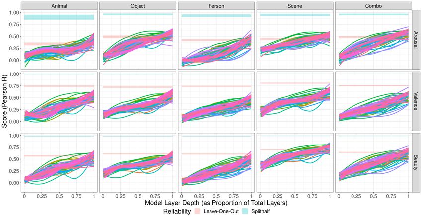
                                                  7

Figure 2: Boxplots comparing how well individual human subjects (in red) predict average human
ratings versus ImageNet-trained and randomly-initialized models (in green and blue, respectively).
Each point in red constitutes the predictions of an individual subject for the rest of the group – also
called the leave-one-out reliability. Each point in green and blue constitutes the best prediction
(the max score across layers) of an individual model from the regularized linear regression fit to
the data from all subjects. The overall takeaways from these plots are threefold: first, ImageNet-
trained models are often as good (or slightly better) than the most group-predictive human subject
(though the absolute value of this advantage may be slightly less given the leave-one-out nature
of the oracle reeliability); second, randomly-initialized models are categorically outperformed by
their ImageNet-trained counterparts; third, beauty, once again, demonstrates what might be called a
goldilocks predictability – with arousal sporting lower scores overall and valence never only slightly
better (on average) than the most group-predictive human subjects.

Figure 3: Rankings of the taskonomy models across all 3 categories of affect in the Oasis dataset. On
the x axis is the model’s max score (the pearson correlation coefficient between the ratings predicted
made by the model’s most predictive layer and the actual ratings provided by the human subjects. On
the y axis is the training task. Notice that object and scene classification dominate in all 3 categories.

                                                    8

References
 [1] Gabriel Kreiman. Biological and Computer Vision. Cambridge University Press, 2021.
 [2] Daniel LK Yamins, Ha Hong, Charles F Cadieu, Ethan A Solomon, Darren Seibert, and James J
     DiCarlo. Performance-optimized hierarchical models predict neural responses in higher visual
     cortex. Proceedings of the National Academy of Sciences, 111(23):8619–8624, 2014.
 [3] Brenden M Lake, Tomer D Ullman, Joshua B Tenenbaum, and Samuel J Gershman. Building
     machines that learn and think like people. Behavioral and brain sciences, 40, 2017.
 [4] Ayse Ilkay Isik and Edward A Vessel. From visual perception to aesthetic appeal: Brain
     responses to aesthetically appealing natural landscape movies. Frontiers in Human Neuroscience,
     page 414, 2021.
 [5] Christoph Redies, Maria Grebenkina, Mahdi Mohseni, Ali Kaduhm, and Christian Dobel.
     Global image properties predict ratings of affective pictures. Frontiers in Psychology, 11:953,
     2020.
 [6] Martin Skov and Marcos Nadal. There are no aesthetic emotions: Comment on menninghaus et
     al.(2019). 2020.
 [7] Winfried Menninghaus, Valentin Wagner, Eugen Wassiliwizky, Ines Schindler, Julian Hanich,
     Thomas Jacobsen, and Stefan Koelsch. What are aesthetic emotions? Psychological review,
     126(2):171, 2019.
 [8] Daniel Graham.       The use of visual statistical features in empirical aesthetics.
     The Oxford Handbook of Empirical Aesthetics. Oxford University Press. https://doi.
     org/10.1093/oxfordhb/9780198824350.013, 19, 2019.
 [9] Anjan Chatterjee. The aesthetic brain: How we evolved to desire beauty and enjoy art. Oxford
     University Press, 2014.
[10] Stephen E Palmer, Karen B Schloss, and Jonathan Sammartino. Visual aesthetics and human
     preference. Annual review of psychology, 64:77–107, 2013.
[11] Rolf Reber. Processing fluency, aesthetic pleasure, and culturally shared taste. Aesthetic science:
     Connecting minds, brains, and experience, pages 223–249, 2012.
[12] Philip A Kragel, Marianne C Reddan, Kevin S LaBar, and Tor D Wager. Emotion schemas are
     embedded in the human visual system. Science advances, 5(7):eaaw4358, 2019.
[13] Kiyohito Iigaya, Sanghyun Yi, Iman A Wahle, Koranis Tanwisuth, and John P O’Doherty.
     Aesthetic preference for art can be predicted from a mixture of low-and high-level visual
     features. Nature Human Behaviour, 5(6):743–755, 2021.
[14] Benedek Kurdi, Shayn Lozano, and Mahzarin R Banaji. Introducing the open affective stan-
     dardized image set (oasis). Behavior research methods, 49(2):457–470, 2017.
[15] Aenne A Brielmann and Denis G Pelli. Intense beauty requires intense pleasure. Frontiers in
     psychology, 10:2420, 2019.
[16] Adam Paszke, Sam Gross, Francisco Massa, Adam Lerer, James Bradbury, Gregory Chanan,
     Trevor Killeen, Zeming Lin, Natalia Gimelshein, Luca Antiga, Alban Desmaison, Andreas
     Kopf, Edward Yang, Zachary DeVito, Martin Raison, Alykhan Tejani, Sasank Chilamkurthy,
     Benoit Steiner, Lu Fang, Junjie Bai, and Soumith Chintala. Pytorch: An imperative style, high-
     performance deep learning library. In H. Wallach, H. Larochelle, A. Beygelzimer, F. d'Alché-
     Buc, E. Fox, and R. Garnett, editors, Advances in Neural Information Processing Systems 32,
     pages 8024–8035. Curran Associates, Inc., 2019. URL http://papers.neurips.cc/paper/
     9015-pytorch-an-imperative-style-high-performance-deep-learning-library.
     pdf.
[17] Ross Wightman.    Pytorch image models.                    https://github.com/rwightman/
     pytorch-image-models, 2019.

                                                   9

[18] Amir R Zamir, Alexander Sax, William Shen, Leonidas J Guibas, Jitendra Malik, and Silvio
     Savarese. Taskonomy: Disentangling task transfer learning. In Proceedings of the IEEE
     Conference on Computer Vision and Pattern Recognition, pages 3712–3722, 2018.
[19] Alexander Sax, Bradley Emi, Amir R. Zamir, Leonidas J. Guibas, Silvio Savarese, and Jitendra
     Malik. Mid-level visual representations improve generalization and sample efficiency for
     learning visuomotor policies. 2018.
[20] Alexander Sax, Jeffrey O Zhang, Bradley Emi, Amir Zamir, Silvio Savarese, Leonidas Guibas,
     and Jitendra Malik. Learning to navigate using mid-level visual priors. arXiv preprint
     arXiv:1912.11121, 2019.
[21] Ryan M Rifkin and Ross A Lippert. Notes on regularized least squares. 2007.
[22] F. Pedregosa, G. Varoquaux, A. Gramfort, V. Michel, B. Thirion, O. Grisel, M. Blondel,
     P. Prettenhofer, R. Weiss, V. Dubourg, J. Vanderplas, A. Passos, D. Cournapeau, M. Brucher,
     M. Perrot, and E. Duchesnay. Scikit-learn: Machine learning in Python. Journal of Machine
     Learning Research, 12:2825–2830, 2011.
[23] Lisa Feldman Barrett and Moshe Bar. See it with feeling: affective predictions during object
     perception. Philosophical Transactions of the Royal Society B: Biological Sciences, 364(1521):
     1325–1334, 2009.

                                                10