The Long-Run Impact of Biofuels on Food Prices - Ujja ya nt Cha kra vort y, Mari e-Hélè ne Hubert, Mic hel M ore aux, and Li nda Nøstbakk en ...
←
→
Page content transcription
If your browser does not render page correctly, please read the page content below
DISCUSSION PAPER
October 2015 RFF DP 15-48
The Long-Run
Impact of Biofuels
on Food Prices
Ujjayant Chakravorty, Marie-Hélène Hubert,
Michel Moreaux, and Linda Nøstbakken
1616 P St. NW
Washington, DC 20036
202-328-5000 www.rff.org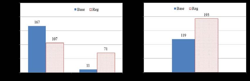
The Long-Run Impact of Biofuels on Food Prices
  Ujjayant Chakravorty, Marie-Hélène Hubert, Michel Moreaux, and Linda Nøstbakken

Abstract
         More than 40 percent of US corn is now used to produce biofuels, which are used as substitutes
for gasoline in transportation. Biofuels have been blamed universally for past increases in world food
prices, and many studies have shown that energy mandates in the United States and European Union may
have a large (30–60 percent) impact on food prices. In this paper, we use a partial equilibrium framework
to show that demand-side effects—in the form of population growth and income-driven preferences for
meat and dairy products rather than cereals—may play as much of a role in raising food prices as biofuels
policy. By specifying a Ricardian model with differential land quality, we find that a significant amount
of new land will be converted to farming, which is likely to cause a modest increase in food prices.
However, biofuels may actually increase aggregate world carbon emissions, due to leakage from lower oil
prices and conversion of pasture and forest land to farming.

Key Words: clean energy, food demand, land quality, renewable fuel standards, transportation

JEL Classification Numbers: Q24, Q32, Q42

© 2015 Resources for the Future. All rights reserved. No portion of this paper may be reproduced without
permission of the authors.
Discussion papers are research materials circulated by their authors for purposes of information and discussion.
They have not necessarily undergone formal peer review.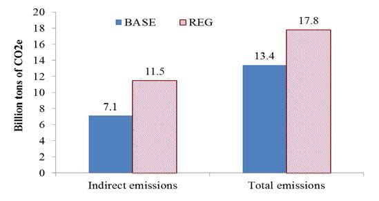
Contents

1. Introduction ......................................................................................................................... 1

2. The Model ............................................................................................................................ 4

3. Calibration of the Model .................................................................................................... 9
     Specification of Demand................................................................................................... 10
     Land Endowment and Productivity .................................................................................. 12
     The Energy Sector............................................................................................................. 15
     US and EU mandates ........................................................................................................ 17
     Carbon Emissions ............................................................................................................. 18
     Trade Among Regions ...................................................................................................... 19
     Model Validation .............................................................................................................. 19

4. Simulation Results ............................................................................................................ 21
     Effect of Biofuel Mandates on Food Prices ...................................................................... 21
     Demand Growth Causes Most of the Land Conversion, Nearly All of It in
       Developing Countries ................................................................................................. 23
     Mandates Lead to Big Increases in Biofuel Production, Earlier in Time ......................... 25
     Mandates Reduce Crude Oil Prices and Cause Significant Leakage and
       Direct Emissions ......................................................................................................... 26
     Indirect Carbon Emissions Increase.................................................................................. 27
     Welfare Declines in the Non-regulated Countries ............................................................ 28

5. Sensitivity Analysis ........................................................................................................... 29
     Model Sensitivity to Parameter Values............................................................................. 29
     European Union, Chinese, and Indian Mandates, Scarcity of Oil and Stationary
        Dietary Preferences ..................................................................................................... 30

6. Concluding Remarks ........................................................................................................ 33

References .............................................................................................................................. 35

Appendix: Data Used in Calibration ................................................................................... 40
Resources for the Future Chakravotry et al.
The Long-Run Impact of Biofuels on Food Prices
Ujjayant Chakravorty, Marie-Hélène Hubert, Michel Moreaux, and Linda Nøstbakken ∗
1. Introduction
Biofuels are providing an ever-larger share of transport fuels, even though they have been
universally attacked for not being a “green” alternative to gasoline. In the United States, about 10
percent of gasoline now comes from corn and this share is expected to rise threefold in the near
future if the Renewable Fuel Standard (RFS) is extended. The European Union, India, and China
have aggressive biofuel mandates as well. Studies that have modeled the effect of these policies
on food prices predict large increases, and have been supported by the run-up in commodity
prices in recent years. For example, the International Food Policy Research Institute (Rosegrant
et al. 2008) suggests that prices of certain crops may rise by up to 70 percent by 2020. 1
In this paper, we examine the long-run effects of US and EU biofuel policy in a dynamic,
partial equilibrium setting. 2 Our approach is unique in two respects. It is common knowledge
∗ Ujjayant Chakravorty, Department of Economics, Tufts University, and Resources for the Future,
ujjayant.chakravorty@tufts.edu; Marie-Hélène Hubert, CREM, Department of Economics, University of Rennes 1,
marie-helene.hubert@univ-rennes1.fr; Michel Moreaux, Toulouse School of Economics (IDEI, LERNA),
mmichel@cict.fr; Linda Nøstbakken, Department of Economics, Norwegian School of Economics,
linda.nostbakken@nhh.no.
Acknowledgements: We would like to thank seminar audiences at the AEA Annual Meetings, Berkeley
BioEconomy Conference, Canadian Resource Economics Workshop, SURED, the World Congress of
Environmental Economics Montreal, EAERE, Rennes, Tufts, Toulouse, Paris, Maryland, Wellesley, Guelph, Peking
University, Philippine School of Economics, Resources for the Future, EPA, Virginia Tech, Statistics Norway, ETH
Zurich, Hawaii, Ohio State, Tinbergen Institute, Curtin, Cal State San Luis Obispo, Western Australia and Georgia
Tech. We are grateful to two anonymous referees and the Editor for comments that significantly improved the paper.
We thank the Social Sciences and Humanities Research Council (SSHRC), the French Council of Energy and the
Ph.D. program at TSE (LERNA) for research funding.
1 Other studies have also found a significant impact, although not to the same degree. For example, Roberts and
Schlenker (2013) use weather-induced yield shocks to estimate the supply and demand for calories and conclude
that energy mandates may trigger a rise in world food prices by 20–30%. Hausman, Auffhammer, and Berck (2012)
use structural vector auto-regression to examine the impact of biofuel production in the United States on corn prices.
They find that one third of corn price increases during 2006–2008 (increases that totaled 28%) can be attributed to
the US biofuel mandate. Their short-run estimates are consistent with our prediction that, in the long run, the
impacts may be significantly lower. This is because higher food prices are likely to trigger supply-side responses
only with a time lag, especially if significant land conversion were to occur.
2Both have imposed large biofuel mandates. Other nations such as China and India have also announced biofuel
mandates but their implementation is still in progress. We discuss them later in the paper.
1Resources for the Future Chakravorty et al.
that, as poor countries develop, their diets change in fundamental ways. In particular, they eat
less cereal and more animal protein in the form of meat and dairy products. 3 This fact is
important because producing meat and dairy uses more land than growing corn. 4 Coupled with
global increases in population, these demand shifts should cause an increase in food prices even
without any biofuel policy. Second, many studies assume a fixed supply of land. There is plenty
of land in the world, although of varying quality for food production. Sustained food price
increases will cause new land to be brought under farming but, as we move down the Ricardian
land-quality gradient, costs will rise, which may in turn put an upward pressure on prices. 5 The
model we develop in this paper explicitly accounts for the above effects in a dynamic setting
where we allow for a rising supply curve of crude oil. 6
Figure 1 shows the disparity in meat and cereal consumption between the United States
and China. Chinese per capita meat consumption is about half that of the United States, but
cereal consumption is much higher. These gaps are expected to narrow significantly in the near
future as the Chinese diet gets an increasing share of its calories from animal protein. 7 Income-
induced changes in dietary preferences have been largely ignored in previous economic studies.
Our results show that about half the predicted rise in food prices may be due to changes in diet.
3 For instance, aggregate meat consumption in China has increased 33 times in the last 50 years, yet the country’s
population has only doubled (Roberts and Schlenker 2013).
4 On average, eight kilos of cereals produce one kilo of beef and three kilos of cereals produce one kilo of pork.
5 Significant amounts of new land are currently being converted to farming (Tyner, 2012).
6 Hertel, Tyner and Birur (2010) use a general equilibrium trade model (GTAP) to explore the impact of biofuels
production on world agricultural markets, specifically focusing on US/EU mandatory blending and its effects on
individual countries. They use disaggregated data on world land quality. However, their static framework does not
account for changes in food preferences. Reilly and Paltsev (2009) also develop a static energy model that does not
account for heterogeneity in land quality.
7Although we use China as an example, the trend holds for other countries as well. For example, per capita meat and
dairy consumption in developed nations is about four times higher than in developing countries.
2Resources for the Future Chakravorty et al.
Figure 1. Per Capita Cereal and Meat Consumption in China and
the United States, 1965-2007
Cereal consumption Meat consumption
Note: Chinese cereal consumption excludes grain converted to meat. Source: FAOSTAT.
Because our main premise is that the pressure on food prices will lead to more land
conversion, the model we propose explicitly accounts for the distribution of land by quality. We
use data from the US Department of Agriculture (USDA), which classify land by soil quality,
location, production cost, and current use, as in pasture or forest. With increased use of biofuels,
oil prices will fall, which will lead to leakage in the form of higher oil use by countries with no
biofuel policy. We endogenously determine the world price of crude oil and the extent of this
spatial leakage. 8 We show that biofuel policy may reduce direct carbon emissions (from
combustion of fossil fuels) in the mandating countries but the reduction is largely offset by an
increase in emissions elsewhere. However, indirect emissions (from land use) go up because of
the conversion of pasture and forest land, mainly in developing countries. Aggregate global
greenhouse gas emissions from the US and EU biofuel mandates actually show a small increase.
The main message of the paper is that demand shifts may have as much of a role in the
rise of food prices as biofuel policy. 9 Moreover, this price increase may be significantly lower
because of supply-side adjustments in the form of an increase in the extensive margin. We obtain
these results with assumptions of modest growth rates in the productivity of land and in the
8 Unlike other studies that determine crude oil use in a static setting.
9 Additional biofuel mandates imposed by China and India also have a surprisingly small effect on food prices.
3Resources for the Future Chakravorty et al.
energy sector. General equilibrium effects of these policies, which we do not consider, may
further diminish the price impact of biofuel mandates. By the same token, models that do not
account for supply-side effects of rising food prices will tend to find large impacts.
Section 2 describes the underlying theoretical model. Section 3 reports the data used in
the calibration. Section 4 reports results and in section 5 we discuss sensitivity analysis. Section
6 concludes the paper. The Appendix provides data on the parameters used in the model.
2. The Model
In this section, we present the detailed theoretical structure of the calibration model used
to estimate food prices. Consider a dynamic, partial equilibrium economy in which three goods,
cereals, meat, and transport energy are produced and consumed in five regions respectively
denoted by r (the United States, European Union, other High Income Countries, Medium
Income Countries and Low Income Countries). Time is denoted by subscript t . The regional
consumption of these goods is denoted by qrc (t ), qrm (t ) and qre (t ) where c, m and e denote
cereals, meat, and energy, respectively. Each region faces a downward-sloping inverse demand
function denoted by Drc−1 ( qrc (t ), t ), Drm
−1
( qrm (t ), t ) and Dre−1 ( qre (t ), t ) , respectively. Within each
region, demand for a good is independent of the demand for other goods. Regional demands for
the three consumption goods (cereals, meat, and transport energy) are modeled by means of
Cobb-Douglas demand functions, which shift exogenously over time because of changes in
population, income, and consumer preferences over meat and cereals. Benefits from
consumption are measured in dollars by the Marshallian surplus, that is, the area under the
inverse demand curve. 10
Land is used to supply food and biofuels. It is available in three qualities denoted by
n = {High, Medium, Low} with High being the highest quality. The acreage of land quality n in
region r devoted to cereals, meat, or biofuel production at any time t is given by Lnrc (t ), Lnrm (t )
and by Lnrb (t ) , respectively, where we denote the different land uses by j = {c, m, b} . Let
∑L n n
rj (t ) be the total acreage in use j for land quality n at any time t and L r be the initial land
j
10 The structure of the model is similar to that adopted by Chakravorty, Roumasset and Tse (1997) for a single
region, and by other studies (e.g., Sohngen, Mendelsohn and Sedjo (1999); Fischer and Newell (2008); and Crago
and Khanna (2014)). Nordhaus (1973) pioneered this approach by assuming independent demand functions for the
US transport, commercial, and residential energy sectors.
4Resources for the Future Chakravorty et al.
area by quality available for cultivation. Aggregate land under the three crops cannot exceed the
∑ L=
n
endowment of land, hence n
(t )
rj Lnr (t ) ≤ L r , for all j. Let new land brought under cultivation
j
n
at any time t be denoted by lr (t ), that is, , where dot denotes the time derivative.
The variable lrn (t ) may be negative if land is taken out of production: here we allow only new
land to be brought into cultivation. 11 The regional total cost of bringing new land into cultivation
is increasing and convex as a function of aggregate land cultivated in the region, but linear in the
amount of new land used at any given instant—this cost is given by cr ( Lnr )lrn where we assume
∂cr ∂ 2cr
that n > 0, n 2 > 0. Additional land brought under production is likely to be located in remote
∂Lr ∂Lr
locations. Thus, the greater the land area already under cultivation, the higher the unit cost of
converting new land to farming within a given quality.
n
Let the yield for land quality n allocated to use j be given by k rj . 12 Yields are higher on
higher quality land. 13 Then the output of food or biofuel energy at any time t is given by
∑ krjn Lnrj . Regional production costs are a function of output and assumed to be rising and
n
convex, that is, more area under cereals, meat, or biofuel production implies a higher cost of
production, given by wrj ( ∑ k rjn Lnrj ).
n
Oil is a nonrenewable resource and we assume a single integrated “bathtub” world oil
market as in Nordhaus (2009). Let X be the initial world stock of oil that is used only for
transportation, X (t ) be the cumulative stock of oil extracted until date t and xr (t ) the regional
rate of consumption so that . The unit extraction cost of oil is increasing and
convex with the cumulative amount of oil extracted, denoted by g ( X ) . Thus, total cost of
11 Allowing land to be taken out of production will make the optimization program complicated. When we run our
calibration model, this variable is never zero before the year 2100 except in the United States (where land
conversion is small in any case, as we see later in the paper) and is never zero in any region after the year 2100
because population keeps increasing and diets trend toward more meat and dairy consumption, which is land
intensive. However, if food prices fall because of exogenous technological change, some land may go out of
production in the distant future. However, that is beyond the scope of our analysis.
12 In the calibration model, crops are transformed into end-use commodities (cereals, meat and, biofuels) by means
of a coefficient of transformation (crops into commodities) and a cost of transformation, both linear. Their values are
reported in the Appendix.
13 See Appendix Tables A5 and A6.
5Resources for the Future Chakravorty et al.
extraction is g ( X )∑ xr (t ) . Crude oil is transformed into gasoline by applying a coefficient of
r
transformation ωr so that total production of gasoline is qgr = ωr xr , where stands for
gasoline. 14 Transport fuel is produced from combining gasoline (derived from crude oil) and
biofuels in a convex linear combination using a CES specification, given by
σr
σ r −1 σ r −1 σ r −1
σr σr
=qre π r µrg qrg + (1 − µrg ) qrb where qre is the production of transport fuel, π r is a
constant, qrg , qrb are the quantities of gasoline and biofuel consumed, µrg is the share of oil,
(1 − µrg ) is the share of biofuels in transport fuel, and σ r is the regional elasticity of substitution.
We assume frictionless trade of food commodities and biofuels across regions. Then we
can write the net export demand (regional production net of consumption) for cereals, meat and
biofuels as ∑ k rcn Lnrc − qrc , ∑ k rm
n n
Lrm − qrm and ∑ k rbn Lnrb − qrb , respectively. Transport
n n n
fuel is not traded but blended and consumed domestically.
Given the exogenous shift in demand caused by population growth and changes in
preferences over meat and cereals driven by an increase in GDP per capita, the social planner
maximizes net discounted surplus across regions and over time using a discount rate ρ > 0 . (S)he
chooses the regional acreage allocated to food and biofuel production, the amount of new land
brought under cultivation, the quantity of each food and energy type used, and the quantity of
gasoline used at each time t in each region r . Note that we do not include the externality cost of
carbon emissions from energy or land use in this program. Later, we exogenously impose the
mandates on biofuel production by region (the United States and the European Union) and solve
for the constrained solution. 15 The optimization problem is written as:
∞
− rt
qrj
r
Max e ∑ ∫ Drj ( qrj , t)dqrj − ∑ cr ( Lr )lr − ∑ wrj ( ∑ k rj Lrj ) − g ( X )∑ x dt (1)
Lrnj , q rj , lnr , x r ∫
−1 n n n n
0
r 0 n j n
r
subject to:
14 We include the cost of refining crude oil into gasoline, described in the Appendix.
15In both the unconstrained and constrained models, we compute the aggregate carbon emissions from each
program.
6Resources for the Future Chakravorty et al.
where qrg = ωr xr . The corresponding generalized Lagrangian can be written as:
qrj −1
=L ∑ ∫ Drj ( qrj , t)dqrj − ∑ cr ( Lnr )lrn − ∑ wrj ( ∑ k rjn Lnrj )
r 0
n j n
− g ( X )∑ x r + ∑∑ β rn ( Lnr − ∑ Lnrj ) + q rn lrn − l ∑ xr
r r n j r
+ ∑ n j ∑ ∑ k rjn Lnrj − qrj
j r n
where β rn is the multiplier associated with the static land constraint (2), q rn and l are
multipliers associated with the two dynamic equations (3) and (4), and n j represents the world
price of traded goods (cereals, meat, and biofuels). We get the following first order conditions:
k rjn (n j − wrj ') − b rn ≤=
0( 0if Lnrj > 0),=j {c, m, b}
(7)
prj − n j ≤ =
0( 0if qrj > 0),=j {c, m} (8)
∂qre
pre − n b ≤=
0( 0if qrb > 0)
∂qrb (9)
q rn − cr ( Lnr ) ≤ =
0( 0if lrn > 0)
(10)
∂qre
pre − g ( X ) − l ≤=
0( 0if qrg > 0).
∂qrg (11)
Finally, the dynamics of the co-state variables are given as:
7Resources for the Future Chakravorty et al.
This is a standard optimization problem with a concave objective function because the
demand functions are downward sloping and costs are linear or convex. The constraints are
linear. We can thus obtain a unique, interior solution. 16
Condition (7) suggests that the cultivated land in each region is allocated either to cereals,
meat, and energy production until the price equals the sum of the production cost plus the
shadow value of the land constraint, given by β rn . Equation (8) suggests that the regional price
r
of cereals and meat ( p j ) equals its world price Equation (9) suggests that the price of
∂q
biofuels in each region ( pe ) , weighted by the term re equals its world price (n b ) . Equation
r
∂qrb
(10) indicates that the marginal cost of land conversion equals the dynamic shadow value of the
stock of land q nr . Equation (11) states that the regional price of gasoline ( pre ) weighted by
∂qre
equals its cost augmented by the scarcity rent l . Conditions (12) and (13) give the
∂qrg
dynamic path of the two co-state variables l and q rn .
According to equations (9) and (11), consumption of biofuel and gasoline, respectively, is
∂qre β rn ∂qre
given by pre = wrb '+ n and pre = g ( X ) + l . Hence, the weighted marginal costs of
∂qrb k rb ∂qrg
biofuels and gasoline are equal. A positive quantity of land is allocated to the production of
cereals, meat, and energy. Obviously, rents will be higher on higher-quality land. An increase in
the demand for energy will induce a shift of acreage from food to energy and hence drive up the
price of food, as well as bring more land into cultivation, potentially of a lower quality.
The biofuel mandate is imposed in the model by requiring a minimum level of
consumption of biofuels in transportation at each date until the year 2022. Define the regional
mandate in time T as q rb (T ) , which implies that biofuel use must not be lower than this level at
16 For an analytical solution to a much simpler but similar problem, see Chakravorty, Magne, and Moreaux (2008).
8Resources for the Future Chakravorty et al.
( )
date T . This constraint can be written as qrb (T ) − q rb (T ) ≥ 0. This will lead to an additional
( )
term τ r qrb (T ) − q rb (T ) in the generalized Lagrangian. The new condition for allocating land to
biofuel (modified equations (7) and (9)) will be
∂q
k rbn pre re − wrb' + τ r − β rn ≤ 0,(
= 0if Lnrb > 0) for all n. The shadow price τ r can be interpreted
∂qrb
as the implicit subsidy to biofuels that bridges the gap between the marginal costs of gasoline
and biofuel. It is of course region-specific. The European mandate is a proportional measure,
which prescribes a minimum percentage of biofuel in the transport–fuel mix. This restriction is
q (T )
implemented in the model by writing rb ≥ s(T ) where s (T ) is the mandated minimum share
qre (T )
of biofuels in transport at time T .
Even though the optimization program abstracts from valuing externalities from carbon
emissions, it is important to find out whether carbon emissions decline due to the imposition of
the biofuel mandate. 17 The model tracks direct as well as indirect carbon emissions. Emissions
from gasoline are constant across regions, but emissions from first- and second-generation
biofuels are region-specific and depend on the crop used. Emissions from gasoline occur at the
consumption stage, whereas biofuel emissions occur mainly at the production stage. Finally,
indirect carbon emissions are released by conversion of new land, namely forests and grasslands,
into food or energy crops. This sequestered carbon is released back into the atmosphere. In the
Appendix we detail the assumptions used to compute regional carbon emissions with and
without the biofuel mandate.
3. Calibration of the Model
In this section, we discuss calibration of the model presented above. We aggregate the
countries into three groups as stated earlier, using data on gross national product per capita
(World Bank 2010). These are High, Medium, and Low Income Countries (HICs, MICs and
LICs). Because our study focuses specifically on US and EU biofuel mandates, the HICs are
further divided into three groups—the United States, the European Union, and Other HICs.
There are five regions in all. Table 1 shows average per capita income by region. The MICs
17 Chakravorty and Hubert (2013) analyze the impact of a carbon tax on the transportation sector in the United
States.
9Resources for the Future Chakravorty et al.
consist of fast-growing economies such as China and India that are likely to account for a
significant share of future world energy demand, as well as large biofuel producers like Brazil,
Indonesia, and Malaysia. The LICs are mainly nations in Africa.
Table 1. Classification of Regions by Income (US$)
Regions GDP per capita Major countries
US 46,405 -
EU 30,741 -
Other HICs 36,240 Canada, Japan
MICs 5,708 China, India, Brazil, Indonesia, Malaysia
LICs 1,061 Mostly African countries
Notes: Per capita GDP in 2007 dollars, PPP adjusted. Source: World Bank (2010).
Specification of Demand
We can now describe the three consumption goods—cereals, meat and dairy products,
and transport energy—in more detail. Cereals include all grains, starches, sugar and sweeteners,
and oil crops. Meat and dairy include all meat products and dairy such as milk and butter. For
convenience, we call this group “meat.” We separate cereals from meat because their demands
are subject to exogenous income shocks as specified below. Meat production is also more land-
intensive than cereals. As mentioned above, transport energy is supplied by gasoline and
biofuels. Cereals, meat, and biofuels compete for land that is already under farming as well as
new land that is currently under grassland or forest cover. 18
Regional demand Drj ( Prj , t ) for good j takes the form:
(14)
where Prj (t ) is the output price of good j at time t in dollars, is the regional own-
price elasticity and β rj (t ) the regional income elasticity for good j which varies exogenously
with per capita income, reflecting changes in food preferences; yr (t ) is regional per capita
income, N r (t ) is regional population at time t and Arj is the constant demand parameter for
18Obviously, many other commodities can be included for a more disaggregated analysis, but we want to keep the
model tractable so that the effects of biofuel policy on land use are transparent.
10Resources for the Future Chakravorty et al.
good j , which we calibrate to reproduce the base-year demand for final commodities for each
region. The constant demand parameters are reported in Appendix Table A1. 19 The demand
function in (14) can be thought of as the demand for a representative individual times the
population of the region. Individual demand is a function of the price of the good and income
given by GDP per capita.
As incomes rise, we expect to observe increased per capita consumption of meat relative
to the consumption of cereals, as noted in numerous studies (e.g., Keyzer et al. 2007). We model
this shift toward animal protein by using income elasticities for food that are higher at lower
levels of per capita income. Specifically, income elasticities for the United States, European
Union and Other HICs are taken to be stationary in the model because dietary preferences and
income in these regions are not expected to change significantly over time, at least relative to
developing countries. However, they are likely to vary in the MICs and LICs due to the larger
increase in per capita incomes. The higher the income, the lower is the income elasticity. All
price and income elasticities are specific to each food commodity (e.g., meat, cereals) and taken
from GTAP (Hertel et al. 2008) as described in the Appendix (Tables A1-A3). 20
We account for regional disparities in the growth of population. While the population of
high-income nations (including the United States and European Union) is expected to be fairly
stable over the next century, that of middle-income countries is predicted to rise by about 40
percent by 2050 and more than double for lower-income countries (UN Population Division,
2010). Demand is also impacted by per capita income in each region, which is assumed to
increase steadily over time but at a decreasing rate, as shown in several studies (e.g., Nordhaus
and Boyer 2000). Again, regional differences are recognized, with the highest growth rates in
MICs and LICs. 21
19 Independence of demand for meat and cereals has been assumed in other studies, see Rosegrant et al. (2001) and
Hertel, Tyner, and Birur (2010).
20 Note that not all developing countries have exhibited as large a growth in meat consumption as China. For
example, a third of Indians are vegetarian and a change in their incomes may not lead to dietary effects of the same
magnitude. Moreover, beef and pork are more land-intensive than chicken, the latter being more popular in countries
like India. The distribution of income may also affect this behavior. If it is regressive, the effect on diets may be
limited.
21 Initial population levels and projections for future growth are taken from the United Nations Population Division
(2010). Both world food and energy demands are expected to grow significantly until about 2050, especially in the
MICs and LICs. By 2050, the current population of 6.8 billion people is predicted to reach nine billion. Beyond that
time, population growth is expected to slow, with a net increase of one billion people between 2050 and 2100.
11Resources for the Future Chakravorty et al.
Land Endowment and Productivity
The initial global endowment of agricultural land is 1.5 billion hectares (FAOSTAT). The
regional distribution of land quality is not even, as is evident from Figure 2, which shows land
endowments based on climate and soil characteristics. 22 Most good land is located in higher-
income countries, but Brazil and India also have sizeable endowments of high-quality land.
Initial endowment for each of the three land qualities can be divided into land already under
cultivation and fallow land. 23 As shown in Table 2, more than half of the agricultural land in the
HICs (United States, European Union, and Other HICs) is classified as high quality, while the
corresponding shares are roughly one third for both MICs and LICs. Most land of medium and
low quality is currently fallow in the form of grasslands and forests, and located in MICs and
LICs. Table 2 shows that there is no high-quality land available for new production. Future
expansion must occur only on lower-quality lands. Brazil alone has 25 percent of all available
lands in the MICs and is the biggest producer of biofuels after the United States.
22 Many factors such as irrigation and climate change can affect land quality. For example, investment in irrigation
can improve the productivity of land. In northern regions like Canada and Russia, higher temperatures may cause an
expansion of land suitable for agricultural production; hence, area under medium and low qualities may increase in
the future. The net effect of these factors on the productivity of new land is unclear and left for future work.
However, we do allow for increasing productivity of land over time (see below).
23 See Appendix for details on land classification. According to FAO (2008a), an additional 1.5 billion hectares of
fallow lands could be brought under crop production in the future. This is approximately equal to the total land area
already under cultivation.
12Resources for the Future Chakravorty et al.
Figure 2. Distribution of Land Quality
Notes: Land quality is defined along two dimensions: soil performance and soil resilience. Soil performance refers
to the suitability of soil for agricultural production; soil resilience is the ability of land to recover from a state of
degradation. Land quality I is the highest quality and IX the lowest. In our model, we ignore category VII through
IX which are unsuitable for agricultural production and aggregate the rest into three qualities (categories I and II
become High quality land, III and IV Medium quality land, and V and VI, Low quality land). Source: US
Department of Agriculture; (Eswaran et al. 2003:121).
As in Gouel and Hertel (2006), the unit cost of accessing new land in a region increases
with land conversion. This can be written as:
(15)
where Lrn is the initial endowment of quality n, so that Lrn − Lnr (t ) is the fallow land
available at date t, and are model parameters, positive in value (calibrated from data) and
assumed to be the same across land quality but varying by region (see Appendix Table A4). 24
24 Intuitively, is the cost of converting the first unit of land to agriculture. Conversion costs increase without
bound as the stock of fallow land declines, because the log of the bracketed term is negative.
13Resources for the Future Chakravorty et al.
Table 2. Current Agricultural Land and Endowment of Fallow Land
Land quality US EU Other HICs MICs LICs World
High 100 100 25 300 150 675
Land already under
agriculture Medium 48 32 20 250 250 590
(million ha) Low 30 11 20 243 44 350
Land available for High 0 0 0 0 0 0
farming (incl. fallow Medium 11 8 21 300 300 640
lands)
(million ha) Low 11 8 21 500 500 1040
Sources: Eswaran et al. (2003); FAO (2008a); Fischer and Shah (2010).
Improvements in agricultural productivity are exogenous and allowed to vary by region
and land quality (see Appendix Table A5). All regions are assumed to exhibit increasing
productivity over time, mainly because of the adoption of biotechnology (e.g., high-yielding crop
varieties), access to irrigation and pest management. However, the rate of technical progress is
higher in MICs and LICs because their current yields, conditional on land quality, are low, owing
to a lag in adopting modern farming practices (FAO 2008a). The rate of technical progress is
also likely to be lower for the lowest land quality. Biophysical limitations such as topography
and climate reduce the efficiency of high-yielding technologies and tend to slow their adoption in
low-quality lands, as pointed out by Fischer et al. (2002).
The production cost for product j (e.g. cereal, meat, or biofuel) for a given region is
η2 r
wrj ( t ) = η1r ∑ k rjn Lnrj ( t ) (16)
n
where the term inside brackets is the aggregate production over all land qualities in the
region and η1r and η2r are regional cost parameters. 25 For food and biofuels, we distinguish
between production and processing costs. All crops need to be packaged and processed and, if
they are converted to biofuels, the refining costs are significant. For cereals and meat, we use the
GTAP 5 database, which provides sectoral processing costs by country (see Appendix Table
A7). Processing costs for biofuels are discussed below.
25 The calibration procedure for this equation is explained in the Appendix and regional cost parameters are reported
in Table A6.
14Resources for the Future Chakravorty et al.
The Energy Sector
Transportation energy qe is produced from gasoline and biofuels in a convex linear
combination using a CES specification. For biofuels we model both land-using (first- generation)
biofuels and newer technologies that are less land-using (second generation); the latter are
described in more detail below. First- and second-generation biofuels are treated as perfect
substitutes, but with different unit costs, as in many other studies (Chen et al. 2012). We use
estimates of the elasticity of substitution made by Hertel, Tyner, and Byrur (2010). We calibrate
the constant parameter in the CES production function to reproduce the base-year production of
blending fuel (see Appendix Table A8 for details). 26
For crude oil reserves, both conventional and unconventional oils (e.g., shale) are
included. According to IEA (2011), around 60 percent of crude oil is used by the transportation
sector. From the estimated oil reserves in 2010, we compute the initial stock of oil available for
transportation as 153 trillion gallons (3.6 trillion barrels) (WEC 2010). The unit cost of oil
depends on the cumulative quantity of oil extracted (as in Nordhaus and Boyer 2000) and can be
written as
ϕ3
X (t )
g( X (t ))= ϕ1 + ϕ2 (17)
X
where X (t ) = ∑∑ x r (t ) is the cumulative oil extracted at time t , X is the initial stock
t r
of crude oil, ϕ1 is the initial extraction cost and (ϕ1 + ϕ 2 ) is the unit cost of extraction of the last
unit of oil. The parameters ϕ1 , ϕ 2 and ϕ3 are obtained from Chakravorty et al. (2012). The
initial extraction cost of oil is around $20 per barrel (or $0.50 per gallon) and costs can rise to
$260 per barrel (or $6.50 per gallon) close to exhaustion (see Appendix Table A10). At these
high prices, unconventional oils become competitive.
For each region, we consider a representative fuel: gasoline for the United States and
diesel for the European Union. 27 We further simplify by considering a representative first-
26Transport fuel production is in billion gallons, which is transformed into Vehicle Miles Traveled (VMT) using the
coefficients reported in Table A9.
27 Gasoline represents more than three-quarters of US transport fuel use, whereas diesel accounts for about 60% in
the European Union (WRI 2010). The coefficients of transformation of oil into gasoline and into diesel are reported
in the Appendix.
15Resources for the Future Chakravorty et al.
generation biofuel for each region. This assumption is reasonable because there is only one type
of biofuel that dominates in each region. For example, 94 percent of biofuel production in the
United States is ethanol from corn, while 76 percent of EU production is biodiesel from
rapeseed. Brazil, the largest ethanol producer among MICs, uses sugarcane. Hence, sugarcane is
used as the representative crop for MICs. In the LICs, 90 percent of biofuels are produced from
cassava, although it amounts to less than 1 percent of global production. 28 Table 3 shows the
representative crop for each region and its processing cost in the model base year. 29 Note the
significant difference in costs across crops. These costs are assumed to decline by around 1
percent a year (Hamelinck and Faaij 2006) mainly due to a decrease in processing costs. 30
Table 3. Unit Processing Costs of First-Generation Biofuels
US EU Other HICs MICs LICs
Feedstock Corn Rapeseed Corn Sugar-cane Cassava
(94%) (76%) (96%) (84%) (99%)
Cost ($/gallon) 1.01 1.55 1.10 0.94 1.30
Notes: The numbers in parentheses represent the percentage of first-generation biofuels produced from the
representative crop in the base year, 2007 (e.g., corn). Sources: FAO (2008a); Eisentraut (2010).
We model a US tax credit of 46 cents/gallon, consisting of both state and federal credits
(de Gorter and Just 2010), which is removed from the model in year 2010, as done in other
studies (Chen et al. 2012). EU states have tax credits on biodiesel ranging from 41-81 cents
(Kojima et al. 2007). We include an average tax credit of 60 cents for the European Union as a
whole.
Second-generation biofuels can be divided into three categories depending on the fuel
source: crops, agricultural residue, and non-agricultural residue. They currently account for only
about 0.1 percent of total biofuel production, although the market share may increase with a
28 Energy yield data for first-generation biofuels are reported in Appendix Table A11.
29 The total cost of biofuels is the sum of the production and processing costs plus rent to land net the value of by-
products. Note that production costs depend on what type of land is being used and in which geographical region,
and land rent is endogenous. By-products may have significant value because only part of the plant (the fruit or the
grain) is used to produce first-generation biofuels. For example, crushed bean “cake” (animal feed) and glycerine are
by-products of biodiesel that can be sold separately. The costs shown in table represent about 50% of the total cost
of production.
30 Except for cassava, for which we have no data.
16Resources for the Future Chakravorty et al.
reduction in costs and improved fuel performance and reliability of the conversion process.
Compared to first-generation fuels, they emit fewer greenhouse gases and are less land
consuming. Among several second-generation biofuels, we model the one that has the highest
potential to be commercially viable in the near future, namely cellulosic ethanol (from
miscanthus, which is a type of perennial grass that produces biofuel) in the United States and
biomass-to-liquid (BTL) fuel in the European Union (IEA 2009b). Their energy yields are much
higher than for first-generation biofuels. In the United States, 800 gallons of ethanol (first
generation) are obtained by cultivating one hectare of corn, while 2,000 gallons of ethanol
(second generation) can be produced from ligno-cellulosic biomass (Khanna 2008). In the
European Union, around 1,000 gallons/ha can be obtained from BTL, but only 400 gallons/ha are
obtained from first-generation biofuels.
Second-generation biofuels are more costly to produce. The processing cost of cellulosic
ethanol is $3.00 per gallon, whereas first-generation corn ethanol currently costs about $1.01 per
gallon and ethanol from sugarcane costs $0.94. 31 The processing cost of BTL diesel is $3.35 per
gallon—twice that of first-generation biodiesel. However, technological progress is expected
gradually to narrow these cost differentials and, by about 2030, the per-gallon processing costs of
second-generation biofuels and BTL diesel are projected to be $1.09 and $1.40, respectively. 32
Finally, second-generation biofuels enjoy a subsidy of $1.01 per gallon in the United States
(Tyner 2012), which is also accounted for in the model.
US and EU mandates
The US mandate sets the domestic target for biofuels at nine billion gallons annually by
2008, increasing to 36 billion gallons by 2022. 33 The bill specifies the use of first- and second-
31 For second-generation biofuels, processing is more costly than for first-generation biofuels and production costs
plus land rent account for about 65% of the total cost.
32Second-generation biofuels costs are assumed to decrease by 2% per year. All data on production costs are from
IEA (2009b).
33 It is not clear whether the mandates will be imposed beyond 2022 but, in our model, we assume that they will be
extended until 2050. In fact, ethanol use in the United States has already hit the 10% “blending wall” imposed by
clean air regulations, which must be relaxed to allow further increases in biofuel consumption. We abstract from
distinguishing among the three categories of advanced biofuels in the US mandate. Of the 21 billion gallons of
second-generation biofuels mandated, four billion gallons are low-emission biofuels that can be met by biofuels
other than cellulosic biofuel, such as sugarcane ethanol imported from Brazil. Another billion gallons may be met by
biodiesel, which is used mainly for trucks. In this study, we assume that the entire target for advanced biofuels has to
be met by cellulosic ethanol.
17Resources for the Future Chakravorty et al.
generation biofuels (respectively, corn ethanol and advanced biofuels), as shown in Figure 3. The
former are scheduled to increase steadily from the current annual level of 11 billion gallons to 15
billion gallons by 2015. The bill requires an increase in the consumption of “advanced” biofuels
(or second-generation biofuels) from near zero to 21 billion gallons per year in 2022. In the
European Union, the mandate requires a minimum biofuels share of 10 percent in transport fuel
by 2020. Unlike the United States, the European Union has no regulation on the use of second-
generation fuels.
Figure 3. US Biofuel Mandate
Carbon Emissions
The model accounts for direct carbon emissions from fossil-fuel consumption in
transportation and indirect carbon emissions induced by the conversion of new land to
agriculture. Carbon from biofuel use is mainly emitted during production and hence is crop-
specific. Considering only direct emissions, displacement of gasoline by corn ethanol reduces
emissions by 35 percent, but displacement of gasoline by ethanol from sugarcane reduces
emissions by 70 percent. Second-generation biofuels reduce carbon emissions by 80 percent
compared to gasoline (Chen et al. 2012). 34 Conversion of land for farming also releases carbon
into the atmosphere. 35 Using Searchinger et al. (2008), we assume that the carbon released
34 Carbon emissions from gasoline and representative biofuels are reported in the Appendix (Table A12).
35 This is a gradual process. For forests, it may also depend on the final use of forest products. However, we assume
that all carbon is released immediately following land-use change, an assumption also made in other well-known
studies (e.g., Searchinger, et al. 2008).
18Resources for the Future Chakravorty et al.
immediately after land conversion is 300 and 500 tons of CO2e (CO2 equivalent) per hectare, for
medium- and low-quality land, respectively. This is because medium-quality land has more
pasture and less forest than low-quality land and, when cleared, pastures emit less carbon than
forests. 36
Trade Among Regions
Although we assume frictionless trading in crude oil and food commodities among
countries, in reality, there are significant trade barriers in agriculture. Given the level of
aggregation in our model, it is difficult to model agricultural tariffs, which are mostly
commodity-specific (sugar, wheat, and so on). However, we do model US and EU tariffs on
biofuels. The US ethanol policy includes a per-unit tariff of $0.54 per gallon and a 2.5 percent ad
valorem tariff (Yacobucci and Schnepf, 2007). The European Union specifies a 6.5 percent ad
valorem tariff on biofuel imports (Kojima et al. 2007). After 2012, US trade tariffs are removed
from the model to match current policy (Economist, 2012).
The discount rate is assumed to be 2 percent, which is standard in such analyses
(Nordhaus and Boyer 2000). We simulate the model over 200 years (2007–2207) in steps of five,
to keep the runs tractable. It is calibrated for the base year 2007. The theoretical framework is
defined as an infinite horizon problem. However, for tractability, we use a finite approximation
in the form of a long time horizon (2007–2207) to ensure that the dynamic rent of oil is positive.
This does not really affect the period of primary interest, which is roughly the next decade. We
follow Sohngen and Mendelsohn (2003) in assuming that exogenous parameters like population
and income do not change significantly after 2100.
Model Validation
It is not possible to test model predictions over a long time horizon because biofuel
mandates have been imposed only recently. However, as shown in Figure 4, the model does track
US gasoline consumption quite closely from 2000 to 2007. 37 The average difference between
36There have been recent studies (see Hertel et al. 2010), which suggest that the emissions from indirect land use
change are likely to be somewhat smaller than those assumed by Searchinger. However, given that significant land-
use change occurs in both our base and regulation models, these new estimates are unlikely to affect the central
conclusions of our paper. Emission levels may change, not the net effect of biofuel regulation.
37 Note that we impose only biofuel mandates in our model so the gasoline consumption is determined
endogenously.
19Resources for the Future Chakravorty et al.
observed and projected values is systematically around 3 percent. The model predicts the annual
average increase in food prices from 2000 to 2013 at 9 percent. 38 According to the FAO, food
prices grew at an annual rate of 7.5 percent during this period. The model solution suggests that
around 19 million hectares of new land are converted for farming from 2000 to 2009. According
to FAOSTAT, 21 million hectares of land were brought into cultivation during this period. These
indicators suggest that the model performs reasonably well in predicting the impact of the
mandates on different variables of interest.
Figure 4. Model Prediction versus Actual US Oil Consumption, 2000–2013
200
Observed values Predicted values
150
Billion gallons
100
50
0
2002 2003 2004 2005 2006 2007 2008 2009 2010 2011 2012 2013
Notes: The difference between observed and predicted values is higher after 2008 because US gasoline
consumption fell during the recession of 2008–2013. Of course, our partial equilibrium model does not
capture short-run macro-economic fluctuations. Source: Consumption figures are from EIA (2014).
38 Our world food price is the average of cereal and meat prices weighted by the share of each commodity in total
food consumption. In general, it is hard accurately to predict food prices in the short run, because of weather-related
variability (droughts such as the one that occurred in Australia in 2008 or Russia in 2010), currency fluctuations, and
other macroeconomic phenomena.
20Resources for the Future Chakravorty et al.
4. Simulation Results
We first state the scenarios modeled in the paper and then describe the results. In the
Baseline case (model BASE), we assume that there are no energy mandates and that both first-
and second-generation fuels are available. This is the unconstrained model described before, and
it serves as the counterfactual. The idea is to see how substitution into biofuels takes place in the
absence of any clean-energy regulation. In the Regulatory Scenario (model REG), US/EU
mandatory blending policies, as described earlier, are imposed. The key results are as follows. 39
Effect of Biofuel Mandates on Food Prices
We find that the effect of the mandates on food prices is significant, but not huge (see
REG in Table 4). With no energy mandates, food prices rise by about 15 percent, which results
purely from changes in population and consumption patterns (see BASE). 40 With energy
mandates, they go up by 32 percent (see REG). Thus, the additional food-price increase in 2022
that results from energy regulation is about 17 percent. 41 This is much smaller than the increase
predicted by the majority of other studies (Rosegrant et al. 2008; Roberts and Schlenker 2012). 42
Figure 5 shows the time trend in food prices under the two regimes. Note that prices
increase both with and without regulation. 43 The substantial increase in food demand in MICs
39 Our results are time-sensitive but, to streamline the discussion, we focus mainly on the year 2022. In the more
distant future (say around 2050 and beyond), rising energy prices and a slowdown in demand growth make biofuels
economical, even without any supporting mandates. Mandates become somewhat redundant by then. Given the lack
of space, we do not discuss what happens in 2050 and beyond.
40 The model is calibrated to track real food prices in 2007. Cereal and meat prices for that year in the BASE case
are $218 and $1,964 per ton, respectively. Observed prices in 2007 were $250 and $2,262, respectively (World Bank
2010). The small difference can be explained by our calibration method, which is based on quantities not prices.
41 Because the model is dynamic, the initial values are endogenous; therefore the starting prices in 2007 are not
exactly equal (Table 4).
42 In general, it is difficult to compare outcomes from different models, but Rosegrant et al. (2008) predict prices of
specific crops such as oilseeds, maize, and sugar rising by 20–70% in 2020, which is generally much higher than in
our case. Roberts and Schlenker (2013) project that 5% of world caloric production would be used for ethanol
production because of the US mandate. As a result, world food prices in their model rise by 30%. These studies
assume energy equivalence between gasoline and biofuels, that is, one gallon of gasoline is equivalent to one gallon
of biofuel. We account for the fact that a gallon of ethanol yields about one third less energy than a gallon of
gasoline, as in Chen et al. (2012).
43Although real food prices have declined in the past four decades, the potential for both acreage expansion and
intensification of agriculture through improved technologies is expected to be lower than in the past (Ruttan 2002).
From 1960 to 2000, crop yields have more than doubled (FAO 2003). However, over the next five decades, yields
are expected to increase by only about 50%: see data presented in Appendix (Table A5). However, yields may also
21Resources for the Future Chakravorty et al.
and LICs, accompanied by a change in dietary preferences, raises the demand for land, which
drives up its opportunity cost. Without energy regulation, meat consumption in these two regions
increases by
Table 4. World Food, Biofuel and Gasoline Prices (in 2007 Dollars)
BASE REG
Weighted food price 2007 557 564
($/ton) 2022 639 (15%) 746 (32%)
Biofuel price 2007 2.14 2.18
($/gallon) 2022 1.97 2.19
Crude oil price 2007 105 106
($/barrel) 2022 121 119
Notes: Weighted food price is the average of cereal and meat prices weighted by the share of each
commodity in total food consumption. The numbers in brackets represent the percentage change in prices
between 2007 and 2022. Our predictions for crude oil prices are quite close to the US Department of
Energy (EIA 2010, 28) reference projection of $115/barrel in 2022: see their “High and Low Oil Price”
range.
8 percent (for MICs) and 34 percent (for LICs) between 2007 and 2022, with the latter
starting from a lower base. The consumption of cereals remains stable. Because more land is
used per kilogram of meat produced, the overall effect is increased pressure on land. Food prices
decline over time as the effects of the mandates wear off. 44 This is mainly because population
growth levels off and yields increase, due to technological improvements in agriculture.
respond to higher food prices, an effect we do not capture here. That would imply a smaller impact of energy
mandates on food prices.
44 The increase in price due to regulation is about 6% in the year 2100.
22Resources for the Future Chakravorty et al.
Figure 5. World Weighted Food Prices
Notes: The baseline model is in blue and the regulated model in red. The weighted food price is the average of
cereal and meat prices weighted by the share of each commodity in total food consumption.
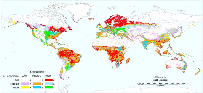
Demand Growth Causes Most of the Land Conversion, Nearly All of It in
Developing Countries
Table 5 shows that the really big increases in land use occur even without mandates: in
the MICs, 119 million ha (= 912 – 793) are brought under production between 2007 and 2022
without any mandates (see BASE). This is about two thirds of all the cultivated land currently in
production in the United States. No new land (including land available under the US
Conservation Reserve Program) is brought under cultivation in the United States because
conversion costs are higher than in MICs. With the mandates, MICs bring another 74 (= 986 –
912) million hectares under farming. Food production in the United States and European Union
declines but rises in the MICs. Overall, the mandates increase aggregate land area in agriculture,
because of conversion of new land.
Table 5. Land Allocation to Food and Energy Production (Million Ha)
US EU MICs
BASE REG BASE REG BASE REG
Land under food 2007 166 167 138 136 789 789
production 2022 166 107 137 129 905 980
Land under 2007 12 11 5 7 4 4
biofuel production 2022 12 71 6 14 7 6
Total 2007 178 178 143 143 793 793
cultivated land 2022 178 178 143 143 912 986
Notes: Land allocation in Other HICs and LICs are similar across the two models.
23You can also read