Studying and Exploiting the Relationship Between Model Accuracy and Explanation Quality
←
→
Page content transcription
If your browser does not render page correctly, please read the page content below
Studying and Exploiting the Relationship Between
        Model Accuracy and Explanation Quality

Yunzhe Jia1       , Eibe Frank1,2 , Bernhard Pfahringer1,2 , Albert Bifet1,3 , and Nick Lim1
                1
                  AI Institute, University of Waikato, Hamilton, New Zealand
     2
         Department of Computer Science, University of Waikato, Hamilton, New Zealand
                           3
                              LTCI, Télécom Paris, IP Paris, France
             {ajia,eibe,bernhard,abifet,nlim}@waikato.ac.nz

         Abstract. Many explanation methods have been proposed to reveal insights about
         the internal procedures of black-box models like deep neural networks. Although
         these methods are able to generate explanations for individual predictions, little
         research has been conducted to investigate the relationship of model accuracy and
         explanation quality, or how to use explanations to improve model performance.
         In this paper, we evaluate explanations using a metric based on area under the
         ROC curve (AUC), treating expert-provided image annotations as ground-truth ex-
         planations, and quantify the correlation between model accuracy and explanation
         quality when performing image classifications with deep neural networks. The
         experiments are conducted using two image datasets: the CUB-200-2011 dataset
         and a Kahikatea dataset that we publish with this paper. For each dataset, we
         compare and evaluate seven different neural networks with four different explain-
         ers in terms of both accuracy and explanation quality. We also investigate how
         explanation quality evolves as loss metrics change through the training iterations
         of each model. The experiments suggest a strong correlation between model ac-
         curacy and explanation quality. Based on this observation, we demonstrate how
         explanations can be exploited to benefit the model selection process—even if
         simply maximising accuracy on test data is the primary goal.

         Keywords: interpretability · explainability · explanation quality

1   Introduction
Interpretability is considered an important characteristic of machine learning models, and
it can be as crucial as accuracy in domains like medicine, finance, and criminal analysis.
Recently, many methods [19, 21, 22, 25, 26] have been proposed to generate visual
explanations for deep neural networks. Since both model accuracy and explanations
are relevant for many practical applications of deep neural networks, it is important
to study the relationship between them. This is challenging because (1) the lack of
ground truth for explanations makes it difficult to quantify their quality—the evaluation
of explanations is generally considered subject to users’ visual judgement—and (2) no
universal measurement has been agreed upon to evaluate explanations. Our work aims
to address this problem and provide empirical results studying the correlation between
model accuracy and explanation quality. Based on the observation that model accuracy
and explanation quality are correlated, we examine a new model selection criterion
combining both model accuracy and explanation quality on validation data.
2 Y. Jia et al.
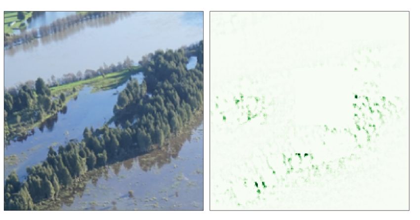
Fig. 1: Demonstration of different explanations by different models making the same
prediction. From top-left to bottom-right: the original image with Kahikatea highlighted
in the red region, the explanations from ResNet18, ResNet50, AlexNet, DenseNet,
InceptionV3, SqueezeNet, and VGG11 generated by the Guided GradCAM explainer.
1.1 Why it is important to evaluate the quality of explanations?
Intuitively, a model that achieves competitive predictive performance and makes deci-
sions based on reasonable evidence is better than one that achieves the same level of
accuracy but makes decisions based on circumstantial evidence. Given a mechanism for
extracting an explanation from a model, we can investigate what evidence the model
uses for generating a particular prediction. If we consider the explanation to be of high
quality if it is based on reasonable evidence and of low quality otherwise, we can attempt
to use explanation quality to inform selection of an appropriate model.
An example of comparing models from the perspective of explanations is shown
in Fig. 1. Given an image containing Kahikatea trees—a species of coniferous tree
that is endemic to New Zealand—seven deep neural networks (ResNet-18, ResNet-50,
AlexNet, DenseNet, Inception-V3, SqueezeNet and VGG11) correctly flag the presence
of this type of tree in the image, but the explanations are different. For this particular
image, and the visual explanations generated by Guided GradCAM [21] that are shown
in the figure, one can argue that the explanations obtained from AlexNet, Inception-V3,
ResNet-18, and VGG-11 are more reasonable than those from other models because they
more closely align with the part of the image containing the species of tree (the red area
marked in the photo).
If we are able to quantify the quality of an explanation, we can define a score for a
model f with respect to both accuracy and explanation quality as
score(f ) = α · scoreacc (f ) + (1 − α) · scoreexplanation (f ) (1)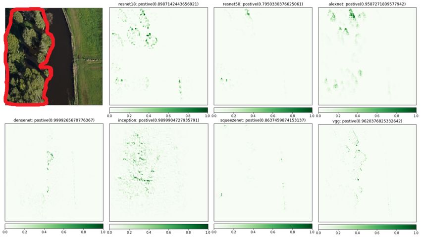
Model Accuracy and Explanation Quality          3

and use it for model selection instead of plain accuracy. Here, scoreacc represents
the model performance in terms of accuracy, scoreexplanation represents the model
performance in terms of explanation quality, and α ∈ [0, 1] is a user-specified parameter.
    In this paper, we propose a mechanism to measure the quality of explanations
scoreexplanation based on area under the ROC curve and perform a large number of
experiments to test the hypothesis that model accuracy is positively correlated with
explanation quality because a model tends to be accurate when it makes decisions
based on reasonable evidence. Although some recent work [4, 1] makes use of this
intuition, there is no theoretical or empirical proof to support the claim. Our work makes
a complementary contribution aimed to close this gap by providing empirical evidence
for the relationship between model accuracy and explanation quality. We hope this will
boost future research on how to use explanations to improve accuracy. As a first step in
this direction, we use Eq. (1) as the selection criterion to choose deep image classification
models from the intermediate candidates that are available at different epochs during
the training process. The results show that the models chosen by considering the quality
of explanations are consistently better than those chosen based on predictive accuracy
alone—in terms of both accuracy and explanation quality on test data.
    The main contributions of our work are:

    – We show how to use a parameter-free AUC-based metric to evaluate explanation
      quality based on expert-provided annotations.
    – We investigate the relationship between model accuracy and explanation quality by
      empirically evaluating seven deep neural networks and four explanation methods.
    – We demonstrate that explanations can be useful for model selection especially when
      the validation data is limited.
    – We publish a new Kahikatea image dataset together with expert explanations for
      individual images.

2     Background and Related Work

We first review work on explainability in neural networks and existing publications that
consider the evaluation of explanation quality.

2.1    Explainability in neural networks

Early research on explainability of neural networks constructed a single tree to mimic the
behaviour of a trained network [5] and uses the interpretable tree to explain the network.
In contrast, recent research focuses on extracting explanations for individual predictions
and can be categorized into two types of approaches: perturbation-based methods and
gradient-based ones.
    Perturbation-based methods generate synthetic samples of a given input and then
extract explanations from the synthetic vicinity of the input. LIME and its variations [19,
20] train a local interpretable model (a linear model or anchors) from the perturbations.
The approaches in [3, 16] compute Shapley values based on perturbations to represent
explanations, and KernelSHAP [16] estimates Shapley values with the LIME framework.
4        Y. Jia et al.

    Gradient-based methods aim to estimate the gradient of a given input with respect
to the target output or a specific layer, and visualize the gradient as an explanation.
Saliency [23] generate gradients by taking a first-order Taylor expansion at the input
layer. Backpropagation [23] and Guided Backpropagation [25] are proposed to compute
the gradients of the input layer with respect to the prediction results. Class Activation
Mapping (CAM) [31] and its variants Gradient-weighted Class Activation Mapping
(GradCAM) and Guided Gradient-weighted Class Activation Mapping (GuidedGrad-
CAM) [21] produce localization maps in the last intermediate layer before the output
layer using gradients with respect to a specific class label. While perturbation-based
methods are usually model-agnostic and can be applied for any model, gradient-based
methods are often used in neural networks. A detailed discussion and comparison can be
found in [7, 17].

2.2   Evaluating explanation quality

Evaluating explanation quality is a challenging problem and, to the best of our knowl-
edge, there is no universally recognized metric for this, mainly due to the variety of
representations used for explanations. Manual evaluation [19, 21, 12] is commonly used
for image explanations. However, evaluation by simple visual inspection is subject to
potential bias [2]. In contrast, [31] computes top-1 error and top-5 error of the image
segments generated by explanations provided by class activation mapping (CAM) tech-
nique. The publications on LIME [19] and LEAP [11] calculate precision, recall and
F1 score to measure explanation quality. The work in [15, 6] converts the problem of
generating image explanations to the problem of weakly-supervised object detection
and adopts the Intersection over Union (IOU) metric that is used in object detection. All
of these methods suffer from the problem that a user-specified threshold or trade-off
parameter is implicitly assumed in the metrics they employ: top-N error, F-measure, and
IOU. In this paper, we adopt a metric based on Area Under the ROC Curve (AUC) to
evaluate explanation quality, which takes into account false positive and true positive
rate for all possible thresholds, and perform an extensive empirical evaluation based on
a large set of explanation methods and models.

3     Definitions

We first give definitions of key concepts that are used in this paper, focusing on the
context of image classification.

Definition 1. Given an image input x of size (M, N ) and a model f , the explanation
e for the prediction f (x) is represented as a two dimensional array of the same size
(M, N ), where each entry in e is a real number and provides the attribution of the
corresponding pixel in x.

Definition 2. Given an image input x of size (M, N ) and a model f , an explainer is a
procedure that takes x and f as inputs and returns an explanation e for the prediction
f (x).
Model Accuracy and Explanation Quality        5

          Fig. 2: Example of an explanation generated by GuidedGradCAM

                      (a) Original image        (b) Expert explanation

              Fig. 3: Example of expert explanation in Kahikatea dataset

An example of an explanation is given in Fig. 2. Given the image input shown on the left
of Fig. 2, and a trained Resnet18 model [8], which makes the prediction that the input
contains Kahikatea trees, the explanation for this prediction is given on the right of Fig.
2. In this example, the explanation is extracted using the explainer GuidedGradCAM
and is visualized as a heat map.

Definition 3. Given an image input x of size (M, N ), the expert explanation etrue for
x is an image of the same size and contains a subset of pixels of x. The pixels in x
are present in etrue if and only if these pixels are selected by an expert based on their
domain knowledge.

The expert explanations for the Kahikatea dataset introduced in this paper are obtained
by domain experts selecting the pixels that are part of Kahikatea trees; an example is
given in Fig. 3. We also use a second dataset for our experiments in this paper: CUB-
200-2011 [29]. The expert explanations for this dataset are extracted from the bounding
box information that covers the locations of objects; an example is given in Fig. 4. Note
that the expert explanations in this latter dataset may not consist exclusively of relevant
information; however, crucially, all relevant object-specific information is included in
the bounding box.

4   Investigating the Relationship between Model Accuracy and
    Explanation Quality
We now discuss the experimental procedure used in our experiments to test the hypothesis
that model accuracy and explanation quality are strongly related.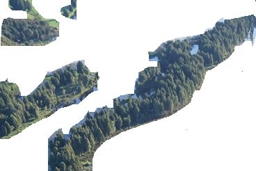
6         Y. Jia et al.

                          (a) Original image       (b) Expert explanation

              Fig. 4: Example of expert explanation in CUB-200-2011 dataset

                     Fig. 5: Process for evaluating the explanation quality

4.1     Evaluating explanation quality
The key step in investigating the relationship between model accuracy and explanation
quality is to quantitatively evaluate the quality of explanations. In this paper, we compute
the Area under the ROC Curve (AUC) to quantify explanation quality because AUC is
scale invariant and threshold invariant.
    Given an image annotated with an expert explanation, and an explanation heat map
generated by an explainer for the prediction of an image by a model, we compute AUC
as follows (the procedure is illustrated in Fig. 5.):
    – Step 1: Convert the expert explanation etrue to a binary two-dimensional matrix
      ebinary
       true , where each entry corresponds to a pixel in the image. The binary value is
      set to 1 if the corresponding pixel is selected in the expert explanation provided for
      the image, and to 0 otherwise.
    – Step 2: Convert the prediction explanation to a two-dimensional matrix e, where
      each entry is the attribution of the corresponding pixel. The attributions are generated
      by an explainer and are normalized into the range [0, 1].
    – Step 3: Flatten both ebinary
                              true   and e into one-dimensional vectors.
    – Step 4: Compute AUC using the ebinary true  and e vectors.
    To show the benefit of using AUC, Fig. 6 shows the comparison of three metrics: pre-
cision, recall and AUC. These metrics are computed for the same generated explanation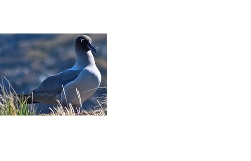
Model Accuracy and Explanation Quality          7

          (a) Original image        (b) Expert explanation    (c) Generated explanation

      (d) Binary explanation with (e) Binary explanation with (f) Binary explanation with
      threshold=0                 threshold=0.1               threshold=0.2

Fig. 6: Comparison of different evaluation metrics. The AUC for (c) is 0.64. (d)-(f) are
the binary explanations that are converted from (c) with different thresholds. Precision
and recall for the binary explanations are as follows: (d) precision=0.29, recall=0.48, (e)
precision=0.66, recall=0.11 , and (f) precision=0.64, recall=0.04

shown in Fig. 6c. To compute precision and recall, a threshold is required to convert the
generated explanation to a binary representation, thus these metrics change as different
thresholds are applied, while AUC is threshold invariant.
    In our experiments, we evaluate the quality of explanations generated by four dif-
ferent explainers from the literature, namely, Saliency [23], BackPropagation [25],
GuidedGradCAM [21], and GradientShap [16].

4.2   Comparing different models

To study the interaction between explainer algorithm and deep neural network that it
is applied to, we evaluate each of the four explainers for seven deep neural networks,
namely, AlexNet [14], DenseNet [9], Inception-V3 [28], ResNet-18 [8], ResNet-50 [30],
SqueezeNet [10], and VGG-11 [24].
    We consider accuracy scoreacc , loss, and explanation quality scoreexplanation . The
primary metric of predictive performance is scoreacc , which is calculated as the por-
tion of correctly classified test instances, but we also report the results of test losses
in the experiments (entropy losses are used for the neural networks in this paper).
scoreexplanation is calculated as the average AUC obtained across all test images.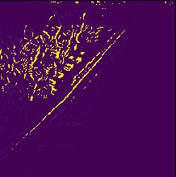
8        Y. Jia et al.

    As illustrated in the example in Fig. 1, it is clear that different models may reach the
same decision based on different evidence—as indicated by the explanations provided.
Thus, it is important to compare models from the perspective of explanation quality,
especially when the models achieve comparable accuracy. However, we can also investi-
gate the correlation between accuracy and explanation quality across different models.
This is important to test the generality of our hypothesis that a model tends to make
correct decisions when its prediction explanations are of high quality.

4.3   Studying explanations as a model evolves during training

It is also of interest to consider how explanations evolve during the training process of
deep neural networks. To this end, instead of just comparing different models, we also
evaluate the explanation quality obtained with a model at different epochs during the
training process.
     Assume a model f is trained with T iterations, and let ft be the intermediate model
at iteration t, scoreexplanation (ft ) be the explanation metric for ft , and scoreacc (ft ) be
the accuracy metric for ft . Then, we compute the correlation between the sequences
of scores [scoreexplanation (f1 ), scoreexplanation (f2 ), . . . , scoreexplanation (fT )] and
[scoreacc (f1 ), scoreacc (f2 ), . . . , scoreacc (fT )] by Pearson correlation that ranges from
-1 (negatively linearly correlated) to 1 (positively linearly correlated) to measure the
strength of the statistical relationship.
     If these two sequences are correlated, it means that the two tasks—learning accurate
classifications and learning accurate explanations—are related. This would provide
some empirical justification for multi-task learning frameworks [4, 1] that jointly learn
classifications and explanations.

4.4   Selecting models based on explanation quality

Assuming model accuracy is positively correlated with explanation quality, it is natural
to consider whether we can choose models based on explanation quality. In the tradi-
tional model selection process, we choose the model that achieves best performance
on validation data and hope it also performs well on test data or unseen data. This
framework usually works if we have a sufficient amount of validation data. However, if
the validation data is limited, a model that performs well on this data will not necessarily
generalise well. In this case, it is worth considering whether the explanation quality on
the validation data (or part of validation data) can be taken into consideration to inform
model selection and thus choose a potentially better model.
    A toy example, considering decision trees rather than neural networks, is given in Fig.
7. Assume there are two trained models (Fig. 7b and Fig. 7c) that perform equally well
on the validation data (Fig. 7a). It is unclear which model will achieve better predictive
accuracy on new data. However, if based on input from domain experts, we know that
features F1 and F2 reflect the actual causes for the class label, then we can say that
model 1 is better than model 2 because its explanation quality is better.
    We explore this idea of using explanation quality for model selection in a case study
with deep neural networks applied to image classification in Section 5.5.
Model Accuracy and Explanation Quality 9
(a) Sample validation data (b) Model 1 (c) Model 2
Fig. 7: Demonstration of how explanations help to choose a better model. Both models
achieve the same accuracy on the validation data. Assuming expert knowledge that F 1
and F 2 are the actual causes for the class label, we can say that model 1 is better than
model 2 as the explanation quality of model 1 is better.
5 Experimental Evaluation
We now discuss the empirical results obtained in our experiments, providing more detail
on the two datasets used and the hardware and software set-up employed.
5.1 Data
The experiments are conducted on two datasets: the CUB-200-2011 dataset and the
Kahikatea dataset. CUB-200-2011 [29] contains 11,788 images (5,994 for training and
5994 for testing) in 200 categories. The images are annotated with bounding boxes reveal-
ing the locations of objects, from where the expert explanations are extracted (see Fig. 4).
The Kahikatea data contains 534 images (426 for training and 108 for testing) in two cat-
egories, and the classification problem is to predict whether an image contains Kahikatea
or not. The expert explanations are generated by domain experts manually selecting the
pixels that belong to Kahikatea trees (see Fig. 3). We publish the Kahikatea dataset with
this paper, and the data can be found at https://doi.org/10.5281/zenodo.5059768.
5.2 Implementation
Our experiments use PyTorch [18] for training the neural networks and Captum [13] for
implementations of the explainers. An NVIDIA GeForce RTX 2070 GPU and an Intel(R)
Core(TM) i7-10750H CPU with 16 GB of memory are used as hardware platform. All
neural networks are trained using the cross-entropy loss function with the SGD [27]
optimizer using batch size = 16, learning rate = 0.001 and momentum = 0.9, while all
explainers are applied with default parameters. The models are trained with 50 epochs
as their performance becomes stable afterwards on the datasets we consider.
5.3 Results - comparing different models
We first compare the models in terms of both classification performance and explanation
quality. The accuracy and loss on the test data for the CUB-200-2011 dataset are reported10 Y. Jia et al.
Model Accuracy Loss EQ-GGCAM EQ-SA EQ-GS EQ-BP
AlexNet 0.495 3.326 0.508 0.507 0.622 0.521
DenseNet 0.764 0.943 0.649 0.641 0.641 0.710
Inception-V3 0.765 0.949 0.662 0.661 0.632 0.661
ResNet-18 0.705 1.141 0.622 0.681 0.644 0.657
ResNet-50 0.758 0.934 0.681 0.687 0.637 0.687
SqueezeNet 0.614 2.090 0.678 0.643 0.644 0.676
VGG-11 0.717 1.371 0.526 0.522 0.650 0.591
Corr(Acc) - - 0.563 0.620 0.516 0.747
Corr(Loss) - - -0.606 -0.691 -0.566 -0.784
Table 1: Comparing models on the CUB-200-2011 data. Explanation quality is shown
for GuidedGradCAM (EQ-GGCAM), Saliency (EQ-SA), GradientShap (EQ-GS), and
BackPropagation (EQ-BP). Corr(Acc): Pearson Correlation between accuracy and expla-
nation quality; Corr(Loss): Pearson Correlation between loss and explanation quality.
Best metrics are shown in bold.
in the second and third column in Table 1. The remaining columns in the table detail the
quality of the explanations generated by the four explainers, measured using AUC. The
correlation between accuracy and explanation quality and the correlation between loss
and explanation quality across these models for each of the four explainers are reported
in the last two rows. Similar results are shown in Table 2 for the Kahikatea dataset.
For both datasets, it can be seen that model accuracy is positively correlated with
explanation quality, while the loss is negatively correlated with explanation quality.
However, it is also worth noting that the model achieving the highest accuracy is not
necessarily the model achieving the best explanation quality. For example, for the
CUB-200-2011 dataset, the Inception-V3 model achieves the highest accuracy, but its
explanation quality is not the best one using any of the explainers—in fact, the ResNet-50
explanations always achieve a better score. This observation highlights the fact that it
may not be advisable to solely rely on accuracy when selecting models in some cases.
5.4 Results - studying a model at different iterations during training
We now investigate the relationship between accuracy and explanation quality for the
intermediate models obtained during the training process. Each model is trained with
50 iterations, which generates 50 intermediate models (including the last iteration).
We compute the accuracy, loss, and explanation quality from four explainers for every
intermediate model. For all intermediate models, we get an accuracy vector of size 50, a
loss vector of size 50, and four explanation quality vectors of size 50. Then, we calculate
the correlations between the accuracy vector and each explanation quality vector, and
the correlations between each loss vector and each explanation quality vector.
The results for the CUB-200-2011 and Kahikatea datasets are reported in Table 3
and Table 4 respectively. It can be seen that during the training process of all seven
models, the accuracy is positively correlated with the explanation quality, and the loss isModel Accuracy and Explanation Quality 11
Model Accuracy Loss EQ-GGCAM EQ-SA EQ-GS EQ-BP
AlexNet 0.926 0.199 0.517 0.542 0.554 0.470
DenseNet 0.981 0.072 0.615 0.587 0.619 0.611
Inception-V3 0.954 0.166 0.526 0.519 0.532 0.472
ResNet-18 0.954 0.137 0.518 0.554 0.563 0.563
ResNet-50 0.972 0.137 0.545 0.566 0.570 0.617
SqueezeNet 0.935 0.227 0.536 0.538 0.558 0.525
VGG-11 0.963 0.118 0.587 0.580 0.600 0.631
Corr(Acc) - - 0.738 0.698 0.669 0.787
Corr(Loss) - - -0.764 -0.791 -0.770 -0.731
Table 2: Comparing models on the Kahikatea data. Explanation quality is shown for
GuidedGradCAM (EQ-GGCAM), Saliency (EQ-SA), GradientShap (EQ-GS), and Back-
Propagation (EQ-BP). Corr(Acc): Pearson Correlation between accuracy and explanation
quality; Corr(Loss): Pearson Correlation between loss and explanation quality. Best
metrics are shown in bold.
GuidedGradCAM Saliency GradientShap BackPropagation
Model Corr(A) Corr(L) Corr(A) Corr(L) Corr(A) Corr(L) Corr(A) Corr(L)
AlexNet 0.707 -0.857 0.842 -0.790 0.827 -0.856 0.786 -0.652
DenseNet 0.840 -0.816 0.903 -0.908 0.759 -0.832 0.738 -0.705
Inception-V3 0.507 -0.603 0.758 -0.802 0.585 -0.661 0.954 -0.934
ResNet-18 0.673 -0.860 0.211 -0.952 0.782 -0.949 0.920 -0.923
ResNet-50 0.921 -0.891 0.891 -0.867 0.974 -0.962 0.905 -0.880
SqueezeNet 0.917 -0.708 0.970 -0.875 0.933 -0.743 0.872 -0.900
VGG-11 0.875 -0.476 0.701 -0.451 0.934 -0.773 0.637 -0.671
Table 3: Results - studying models during training with the CUB-200-2011 dataset.
Corr(A): Pearson Correlation between accuracy and explanation quality; Corr(L): Pear-
son Correlation between loss and explanation quality. Best metrics are shown in bold.
negatively correlated with the explanation quality. This validates our intuition that the
explanation quality improves as the accuracy increases.
5.5 Using Explanations for Model Selection
We now proceed to a case study4 where we investigate whether explanations can be
used to improve the model selection performance in the Kahikatea problem under the
assumption that the validation data is limited.
Given training and validation data, in the traditional model selection setting, can-
didate models (i.e., different models structures, identical model structures trained with
4
The code and supplementary material are available at https://bit.ly/3xdcrwS12 Y. Jia et al.
GuidedGradCAM Saliency GradientShap BackPropagation
Model Corr(A) Corr(L) Corr(A) Corr(L) Corr(A) Corr(L) Corr(A) Corr(L)
AlexNet 0.507 -0.602 0.585 -0.689 0.530 -0.520 0.646 -0.585
DenseNet 0.510 -0.548 0.493 -0.427 0.550 -0.612 0.461 -0.423
Inception-V3 0.358 -0.421 0.475 -0.526 0.780 -0.710 0.576 -0.551
ResNet-18 0.423 -0.350 0.659 -0.460 0.706 -0.548 0.801 -0.562
ResNet-50 0.510 -0.454 0.499 -0.571 0.391 -0.311 0.394 -0.493
SqueezeNet 0.478 -0.281 0.498 -0.387 0.415 -0.535 0.498 -0.421
VGG-11 0.417 -0.511 0.663 -0.469 0.655 -0.384 0.722 -0.521
Table 4: Results - studying models during training with the Kahikatea dataset. Corr(A):
Pearson Correlation between accuracy and explanation quality; Corr(L): Pearson Corre-
lation between loss and explanation quality. Best metrics are shown in bold.
different hyper-parameters, or intermediate models from different training stages) are
obtained on the training data, and the model that achieves the best performance in terms
of accuracy or loss on the validation data is selected to later be applied on test data or
unseen data.
Instead of using the accuracy metric as the selection criterion, we use score(f ) =
α·scoreacc (f )+(1−α)·scoreexplanation (f ) (see Eq. (1)), such that the model with the
best score(f ) on the validation data is selected. This selection criterion is based on our
previous observation that explanation quality and model accuracy are strongly correlated.
scoreexplanation can be viewed as a regularization term regarding explainability, and it
helps to reduce variance and avoid overfitting by choosing models that make decisions
based on reasonable evidence.
It is worth noting that in the case when α = 1, the selection criterion only relies on
accuracy, which is the way traditional model selection makes its choice, whilst in the
case when α = 0, the selection criterion only relies on explainability.
Given the Kahikatea dataset and a deep neural network model structure, we perform
the following steps:
– Step 1: Randomly divide the Kahikatea dataset into three subsets such that 20% of
the samples are for training, 10% are for validation, and the remaining 70% are for
testing.
– Step 2: Train the model on the training data for N = 50 iterations to generate 50
model candidates f1 , f2 , . . . , fN .
– Step 3: Compute score(f ) in Eq. (1) on the validation data for fi , i ∈ [1, 2, . . . , N ],
where scoreacc (fi ) is calculated as the percentage of correct predictions of fi on the
validation data, scoreexplanation (fi ) is calculated using the AUC-based metric (see
Section 4.1) with expert explanations for the validation data and model explanations
generated with GuidedGradCAM.
– Step 4: Compute test accuracy (percentage of correct predictions on the test data)
Acctest (f ) for fi , i ∈ [1, 2, . . . , N ].Model Accuracy and Explanation Quality 13
– Step 5: Calculate the Pearson correlation between (score(f1 ), . . . , score(fN )) and
(Acctest (f1 ), . . . , Acctest (fN )). The correlation is 1 if the ranking of the candidate
models based on score(f ) is the same as their ranking based on test accuracy.
– Step 6: Repeat step 1-5 for 10 times and compute the average correlation.
The procedure is applied on seven deep neural networks (AlexNet, DenseNet,
Inception-V3, ResNet-18, ResNet-50, SqueezeNet and VGG-11) and α is varied from
the list (0, 0.1, 0.2, 0.3, 0.4, 0.5, 0.6, 0.7, 0.8, 0.9, 1.0) to cover both extreme cases.
The correlation between the scores of the selection criterion and test accuracy is
reported in Table 5. It can be seen that, for all models, the highest correlations are
achieved when α is neither 0 nor 1, which suggests that a combination of validation set
accuracy and explanation quality is best for model selection.
α AlexNet DenseNet Inception-V3 ResNet-18 ResNet-50 SqueezeNet VGG-11
0 0.5335 0.5076 0.4602 0.5914 0.4281 0.4448 0.6011
0.1 0.6006 0.5996 0.6393 0.6734 0.5345 0.5426 0.678
0.2 0.6629 0.6807 0.7627 0.7372 0.6289 0.6348 0.7438
0.3 0.717 0.7466 0.8332 0.7838 0.7057 0.7073 0.7947
0.4 0.7587 0.7964 0.8666 0.8156 0.7633 0.7578 0.8305
0.5 0.7844 0.8311 0.88 0.8354 0.8038 0.7899 0.8531
0.6 0.7929 0.8533 0.8834 0.8458 0.8305 0.8077 0.8653
0.7 0.7873 0.8655 0.882 0.8494 0.8465 0.8152 0.8694
0.8 0.7734 0.8703 0.8783 0.8479 0.8545 0.8153 0.8678
0.9 0.7561 0.8698 0.8735 0.8433 0.8568 0.8106 0.8619
1.0 0.7378 0.8657 0.8684 0.8366 0.8553 0.8028 0.8532
Table 5: Results - Correlations of selection scores and test accuracy for different α. Best
metrics for each model are shown in bold.
The comparison of the test accuracy of models selected with explanations and that
of the models selected without explanations is shown in Table 6. When α = 1, it is
the case that we choose the models without considering explanation quality. Besides
the test accuracy, the explanation quality on the test data of models selected with
explanations is consistently better than that of models selected without explanations
(see the supplementary material). It can be seen that the models selected by consulting
explanation quality consistently outperform the models (except for SqueezeNet) selected
using accuracy alone. It also shows that we cannot simply optimize the explanation
quality (when α = 0), and one possible reason is that the expert explanations can be
biased and noisy.
Do we need expert explanations for all validation data? It is interesting to consider
how many instance-level expert explanations are sufficient to improve the performance
of model selection if these are not available for the whole validation set. We follow14 Y. Jia et al.
α AlexNet DenseNet Inception-V3 ResNet-18 ResNet-50 SqueezeNet VGG-11
0 79.95% 81.37% 76.87% 83.08% 82.64% 77.28% 83.71%
0.1 79.97% 81.07% 77.28% 82.99% 82.61% 80.0% 83.71%
0.2 79.97% 82.39% 82.01% 82.8% 82.99% 80.96% 84.59%
0.3 82.01% 82.42% 82.34% 82.69% 83.1% 81.59% 84.78%
0.4 82.06% 82.17% 82.34% 82.99% 83.38% 81.18% 84.64%
0.5 82.06% 82.09% 82.23% 82.99% 83.68% 81.92% 84.64%
0.6 82.06% 82.99% 82.34% 82.94% 83.63% 81.81% 84.09%
0.7 82.06% 83.24% 82.5% 82.99% 83.49% 81.43% 84.42%
0.8 82.06% 83.24% 82.5% 82.99% 83.49% 81.54% 84.45%
0.9 81.54% 83.24% 82.5% 82.99% 83.49% 81.54% 84.45%
1.0 81.18% 82.42% 82.2% 82.72% 83.43% 82.01% 84.42%
Table 6: Results - Test accuracy of models selected using selection criterion with different
α. Best metrics for each model are shown in bold.
the setting described above and vary the availability of expert explanations from 10%
to 100% of the validation set. The model selection result (test accuracy) for AlexNet
with the GuidedGradCAM explainer is shown in Table 7. It can be seen that even with
10% expert explanations it is possible to improve the model selection performance. The
results of other neural network structures (see the supplementary material) follow a
similar trend: availability of expert explanations for 10% of the validation data (or more)
can benefit the model selection process for the selected dataset.
Level of expert explanation availability
α 10% 20% 30% 40% 50% 60% 70% 80% 90% 100%
0 82.3% 81.8% 81.8% 82.0% 81.9% 81.3% 82.0% 80.7% 82.6% 79.9%
0.1 82.3% 81.8% 81.8% 82.0% 81.7% 81.4% 82.0% 80.7% 82.6% 80.0%
0.2 82.3% 82.0% 81.8% 82.0% 81.7% 81.4% 82.0% 80.7% 82.3% 80.0%
0.3 82.3% 82.0% 82.1% 82.0% 81.7% 81.4% 82.0% 81.3% 82.3% 82.0%
0.4 82.1% 82.1% 82.2% 82.0% 82.0% 82.0% 82.0% 82.0% 82.3% 82.1%
0.5 82.1% 82.1% 82.4% 82.0% 82.0% 82.1% 82.0% 82.2% 82.3% 82.1%
0.6 82.1% 82.1% 82.4% 82.2% 81.9% 82.4% 82.1% 82.2% 82.4% 82.1%
0.7 82.2% 82.3% 82.5% 82.2% 82.1% 82.6% 82.1% 82.2% 82.4% 82.1%
0.8 82.4% 81.8% 82.6% 81.8% 81.8% 82.6% 82.2% 82.3% 82.4% 82.1%
0.9 82.0% 81.9% 82.4% 81.8% 81.3% 82.6% 82.2% 81.9% 81.9% 81.5%
1.0 81.2% 81.2% 81.2% 81.2% 81.2% 81.2% 81.2% 81.2% 81.2% 81.2%
Table 7: Results - Test accuracy of models selected with different percentages of expert
explanations. Best results for each model are shown in bold.Model Accuracy and Explanation Quality 15
6 Conclusion
We empirically evaluate the relationship between model accuracy and explanation
quality using seven deep neural networks and four explainers. To evaluate explanation
quality, we adopt the Area under the ROC Curve (AUC), which is threshold invariant.
The experimental results indicate that models tend to make correct predictions when
these predictions are accompanied by explanations of high quality. Moreover, during a
model’s training process, predictive accuracy increases together with explanation quality.
Our results provide strong empirical support for the claim that model accuracy and
explanation quality are correlated. Exploiting this observation, we demonstrate how
measuring the quality of explanations can help to improve the performance of model
selection and also consider how this is affected by the number of available expert-
provided explanations. To boost research in this area, we publish the Kahikatea dataset,
which provides instance-level expert explanations for positive instances.
Acknowledgments
This work is partially supported by the TAIAO project (Time-Evolving Data Sci-
ence / Artificial Intelligence for Advanced Open Environmental Science) funded by
the New Zealand Ministry of Business, Innovation, and Employment (MBIE). URL
https://taiao.ai/. This work is partially supported by Microsoft AI for Earth Grants for
providing cloud computing resource. We thank Waikato Regional Council (WRC) staff
and students that have worked on the Kahikatea project along with further assistance
from Rebecca Finnerty and Paul Dutton for the Kahikatea dataset.
References
1. Avinesh, P., Ren, Y., Meyer, C.M., Chan, J., Bao, Z., Sanderson, M.: J3r: Joint multi-task
learning of ratings and review summaries for explainable recommendation. In: ECML-PKDD.
pp. 339–355 (2019)
2. Buçinca, Z., Lin, P., Gajos, K.Z., Glassman, E.L.: Proxy tasks and subjective measures can be
misleading in evaluating explainable ai systems. In: IUI. pp. 454–464 (2020)
3. Castro, J., Gómez, D., Tejada, J.: Polynomial calculation of the shapley value based on
sampling. Computers & Operations Research 36(5), 1726–1730 (2009)
4. Chen, Z., Wang, X., Xie, X., Wu, T., Bu, G., Wang, Y., Chen, E.: Co-attentive multi-task
learning for explainable recommendation. In: IJCAI. pp. 2137–2143 (2019)
5. Craven, M., Shavlik, J.: Extracting tree-structured representations of trained networks. In:
NIPS. pp. 24–30 (1995)
6. Guidotti, R.: Evaluating local explanation methods on ground truth. Artificial Intelligence
291, 103428 (2021)
7. Guidotti, R., Monreale, A., Ruggieri, S., Turini, F., Giannotti, F., Pedreschi, D.: A survey of
methods for explaining black box models. ACM Computing Surveys 51(5), 1–42 (2018)
8. He, K., Zhang, X., Ren, S., Sun, J.: Deep residual learning for image recognition. In: CVPR.
pp. 770–778 (2016)
9. Huang, G., Liu, Z., Van Der Maaten, L., Weinberger, K.Q.: Densely connected convolutional
networks. In: CVPR. pp. 4700–4708 (2017)16 Y. Jia et al.
10. Iandola, F.N., Han, S., Moskewicz, M.W., Ashraf, K., Dally, W.J., Keutzer, K.:
Squeezenet: Alexnet-level accuracy with 50x fewer parameters and < 0.5 MB model size.
arXiv:1602.07360 (2016)
11. Jia, Y., Bailey, J., Ramamohanarao, K., Leckie, C., Houle, M.E.: Improving the quality of
explanations with local embedding perturbations. In: KDD. pp. 875–884 (2019)
12. Kim, B., Wattenberg, M., Gilmer, J., Cai, C., Wexler, J., Viegas, F., et al.: Interpretability
beyond feature attribution: Quantitative testing with concept activation vectors (TCAV). In:
ICML. pp. 2668–2677 (2018)
13. Kokhlikyan, N., Miglani, V., Martin, M., Wang, E., Alsallakh, B., Reynolds, J., Melnikov, A.,
Kliushkina, N., Araya, C., Yan, S., et al.: Captum: A unified and generic model interpretability
library for PyTorch. arXiv:2009.07896 (2020)
14. Krizhevsky, A.: One weird trick for parallelizing convolutional neural networks.
arXiv:1404.5997 (2014)
15. Lin, Y.S., Lee, W.C., Celik, Z.B.: What do you see? Evaluation of explainable artificial
intelligence (XAI) interpretability through neural backdoors. arXiv:2009.10639 (2020)
16. Lundberg, S.M., Lee, S.I.: A unified approach to interpreting model predictions. In: NIPS. pp.
4765–4774 (2017)
17. Molnar, C.: Interpretable Machine Learning. Lulu. com (2020)
18. Paszke, A., Gross, S., Massa, F., Lerer, A., Bradbury, J., Chanan, G., Killeen, T., Lin, Z.,
Gimelshein, N., Antiga, L., et al.: Pytorch: An imperative style, high-performance deep
learning library. In: NeuRIPS. pp. 8026–8037 (2019)
19. Ribeiro, M.T., Singh, S., Guestrin, C.: “Why should I trust you?” Explaining the predictions
of any classifier. In: KDD. pp. 1135–1144 (2016)
20. Ribeiro, M.T., Singh, S., Guestrin, C.: Anchors: High-precision model-agnostic explanations.
In: AAAI. vol. 18, pp. 1527–1535 (2018)
21. Selvaraju, R.R., Cogswell, M., Das, A., Vedantam, R., Parikh, D., Batra, D.: Grad-CAM:
Visual explanations from deep networks via gradient-based localization. In: ICCV. pp. 618–
626 (2017)
22. Shrikumar, A., Greenside, P., Kundaje, A.: Learning important features through propagating
activation differences. In: ICML. pp. 3145–3153 (2017)
23. Simonyan, K., Vedaldi, A., Zisserman, A.: Deep inside convolutional networks: Visualising
image classification models and saliency maps. arXiv:1312.6034 (2013)
24. Simonyan, K., Zisserman, A.: Very deep convolutional networks for large-scale image recog-
nition. arXiv:1409.1556 (2014)
25. Springenberg, J.T., Dosovitskiy, A., Brox, T., Riedmiller, M.: Striving for simplicity: The all
convolutional net. arXiv:1412.6806 (2014)
26. Sundararajan, M., Taly, A., Yan, Q.: Axiomatic attribution for deep networks. In: ICML. pp.
3319–3328 (2017)
27. Sutskever, I., Martens, J., Dahl, G., Hinton, G.: On the importance of initialization and
momentum in deep learning. In: ICML. pp. 1139–1147 (2013)
28. Szegedy, C., Vanhoucke, V., Ioffe, S., Shlens, J., Wojna, Z.: Rethinking the inception architec-
ture for computer vision. In: CVPR. pp. 2818–2826 (2016)
29. Wah, C., Branson, S., Welinder, P., Perona, P., Belongie, S.: The Caltech-UCSD Birds-200-
2011 Dataset. Tech. Rep. CNS-TR-2011-001, California Institute of Technology (2011)
30. Xie, S., Girshick, R., Dollár, P., Tu, Z., He, K.: Aggregated residual transformations for deep
neural networks. In: CVPR. pp. 1492–1500 (2017)
31. Zhou, B., Khosla, A., Lapedriza, A., Oliva, A., Torralba, A.: Learning deep features for
discriminative localization. In: CVPR. pp. 2921–2929 (2016)You can also read