Skilful precipitation nowcasting using deep generative models of radar
←
→
Page content transcription
If your browser does not render page correctly, please read the page content below
Article

Skilful precipitation nowcasting using deep
generative models of radar

https://doi.org/10.1038/s41586-021-03854-z                       Suman Ravuri1,5, Karel Lenc1,5, Matthew Willson1,5, Dmitry Kangin2,3, Remi Lam1,
                                                                 Piotr Mirowski1, Megan Fitzsimons2, Maria Athanassiadou2, Sheleem Kashem1, Sam Madge2,
Received: 17 February 2021
                                                                 Rachel Prudden2,3, Amol Mandhane1, Aidan Clark1, Andrew Brock1, Karen Simonyan1,
Accepted: 27 July 2021                                           Raia Hadsell1, Niall Robinson2,3, Ellen Clancy1, Alberto Arribas2,4 & Shakir Mohamed1 ✉

Published online: 29 September 2021

Open access                                                      Precipitation nowcasting, the high-resolution forecasting of precipitation up to two
    Check for updates                                            hours ahead, supports the real-world socioeconomic needs of many sectors reliant on
                                                                 weather-dependent decision-making1,2. State-of-the-art operational nowcasting
                                                                 methods typically advect precipitation fields with radar-based wind estimates, and
                                                                 struggle to capture important non-linear events such as convective initiations3,4.
                                                                 Recently introduced deep learning methods use radar to directly predict future rain
                                                                 rates, free of physical constraints5,6. While they accurately predict low-intensity
                                                                 rainfall, their operational utility is limited because their lack of constraints produces
                                                                 blurry nowcasts at longer lead times, yielding poor performance on rarer
                                                                 medium-to-heavy rain events. Here we present a deep generative model for the
                                                                 probabilistic nowcasting of precipitation from radar that addresses these challenges.
                                                                 Using statistical, economic and cognitive measures, we show that our method
                                                                 provides improved forecast quality, forecast consistency and forecast value. Our
                                                                 model produces realistic and spatiotemporally consistent predictions over regions
                                                                 up to 1,536 km × 1,280 km and with lead times from 5–90 min ahead. Using a
                                                                 systematic evaluation by more than 50 expert meteorologists, we show that our
                                                                 generative model ranked first for its accuracy and usefulness in 89% of cases against
                                                                 two competitive methods. When verified quantitatively, these nowcasts are skillful
                                                                 without resorting to blurring. We show that generative nowcasting can provide
                                                                 probabilistic predictions that improve forecast value and support operational utility,
                                                                 and at resolutions and lead times where alternative methods struggle.

The high-resolution forecasting of rainfall and hydrometeors zero to                             used; radar data is now available (in the UK) every five minutes and at
two hours into the future, known as precipitation nowcasting, is crucial                         1 km × 1 km grid resolution11. Established probabilistic nowcasting
for weather-dependent decision-making. Nowcasting informs the                                    methods, such as STEPS and PySTEPS3,4, follow the NWP approach of
operations of a wide variety of sectors, including emergency services,                           using ensembles to account for uncertainty, but model precipitation
energy management, retail, flood early-warning systems, air traffic                              following the advection equation with a radar source term. In these
control and marine services1,2. For nowcasting to be useful in these                             models, motion fields are estimated by optical flow, smoothness pen-
applications the forecast must provide accurate predictions across                               alties are used to approximate an advection forecast, and stochastic
multiple spatial and temporal scales, account for uncertainty and be                             perturbations are added to the motion field and intensity model3,4,12.
verified probabilistically, and perform well on heavier precipitation                            These stochastic simulations allow for ensemble nowcasts from which
events that are rarer, but more critically affect human life and economy.                        both probabilistic and deterministic forecasts can be derived and are
   Ensemble numerical weather prediction (NWP) systems, which                                    applicable and consistent at multiple spatial scales, from the kilometre
simulate coupled physical equations of the atmosphere to generate                                scale to the size of a catchment area13.
multiple realistic precipitation forecasts, are natural candidates for                              Approaches based on deep learning have been developed that move
nowcasting as one can derive probabilistic forecasts and uncertainty                             beyond reliance on the advection equation5,6,14–19. By training these
estimates from the ensemble of future predictions7. For precipitation                            models on large corpora of radar observations rather than relying on
at zero to two hours lead time, NWPs tend to provide poor forecasts as                           in-built physical assumptions, deep learning methods aim to better
this is less than the time needed for model spin-up and due to difficulties                      model traditionally difficult non-linear precipitation phenomena, such
in non-Gaussian data assimilation8–10. As a result, alternative methods                          as convective initiation and heavy precipitation. This class of methods
that make predictions using composite radar observations have been                               directly predicts precipitation rates at each grid location, and models

DeepMind, London, UK. 2Met Office, Exeter, UK. 3University of Exeter, Exeter, UK. 4University of Reading, Reading, UK. 5These authors contributed equally: Suman Ravuri, Karel Lenc, Matthew
1

Willson. ✉e-mail: shakir@deepmind.com

672 | Nature | Vol 597 | 30 September 2021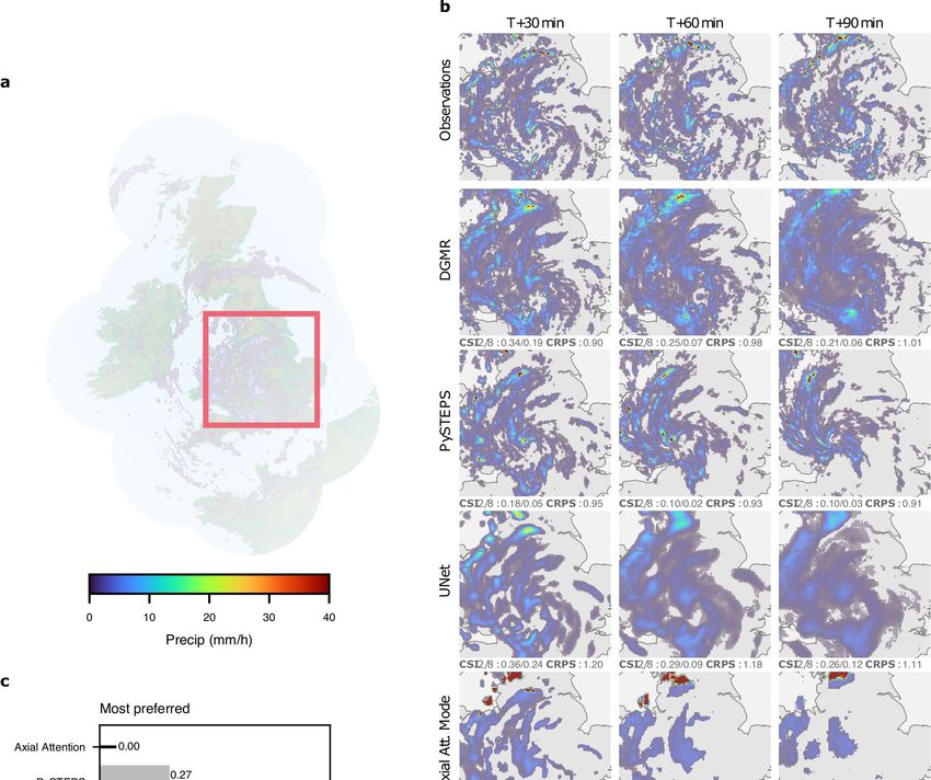
have been developed for both deterministic and probabilistic forecasts.       temporal consistency and penalizes jumpy predictions. These two
As a result of their direct optimization and fewer inductive biases, the      discriminators share similar architectures to existing work in video
forecast quality of deep learning methods—as measured by per-grid-cell        generation26. When used alone, these losses lead to accuracy on par with
metrics such as critical success index (CSI)20 at low precipitation levels    Eulerian persistence. To improve accuracy, we introduce a regulariza-
(less than 2 mm h−1)—has greatly improved.                                    tion term that penalizes deviations at the grid cell resolution between
   As a number of authors have noted5,6, forecasts issued by current deep     the real radar sequences and the model predictive mean (computed
learning systems express uncertainty at increasing lead times with blur-      with multiple samples). This third term is important for the model to
rier precipitation fields, and may not include small-scale weather pat-       produce location-accurate predictions and improve performance.
terns that are important for improving forecast value. Furthermore, the       In the Supplementary Information, we show an ablation study sup-
focus in existing approaches on location-specific predictions, rather         porting the necessity of each loss term. Finally, we introduce a fully
than probabilistic predictions of entire precipitation fields, limits their   convolutional latent module for the generator, allowing for predic-
operational utility and usefulness, being unable to provide simulta-          tions over precipitation fields larger than the size used at training time,
neously consistent predictions across multiple spatial and temporal           while maintaining spatiotemporal consistency. We refer to this DGM
aggregations. The ability to make skilful probabilistic predictions is        of rainfall as DGMR in the text.
also known to provide greater economic and decision-making value                 The model is trained on a large corpus of precipitation events,
than deterministic forecasts21,22.                                            which are 256 × 256 crops extracted from the radar stream, of length
   Here we demonstrate improvements in the skill of probabilistic pre-        110 min (22 frames). An importance-sampling scheme is used to cre-
cipitation nowcasting that improves their value. To create these more         ate a dataset more representative of heavy precipitation (Methods).
skilful predictions, we develop an observations-driven approach for           Throughout, all models are trained on radar observations for the UK
probabilistic nowcasting using deep generative models (DGMs). DGMs            for years 2016–2018 and evaluated on a test set from 2019. Analysis
are statistical models that learn probability distributions of data and       using a weekly train–test split of the data, as well as data of the USA, is
allow for easy generation of samples from their learned distributions.        reported in Extended Data Figs. 1–9 and the Supplementary Informa-
As generative models are fundamentally probabilistic, they have the           tion. Once trained, this model allows fast full-resolution nowcasts to
ability to simulate many samples from the conditional distribution of         be produced, with a single prediction (using an NVIDIA V100 GPU)
future radar given historical radar, generating a collection of forecasts     needing just over a second to generate.
similar to ensemble methods. The ability of DGMs to both learn from
observational data as well as represent uncertainty across multiple
spatial and temporal scales makes them a powerful method for devel-           Intercomparison case study
oping new types of operationally useful nowcasting. These models can          We use a single case study to compare the nowcasting performance of the
predict smaller-scale weather phenomena that are inherently difficult         generative method DGMR to three strong baselines: PySTEPS, a widely
to predict due to underlying stochasticity, which is a critical issue for     used precipitation nowcasting system based on ensembles, considered
nowcasting research. DGMs predict the location of precipitation as            to be state-of-the-art3,4,13; UNet, a popular deep learning method for now-
accurately as systems tuned to this task while preserving spatiotem-          casting15; and an axial attention model, a radar-only implementation of
poral properties useful for decision-making. Importantly, they are            MetNet19. For a meteorologically challenging event, Figs. 1b, c and 4b
judged by professional meteorologists as substantially more accurate          shows the ground truth and predicted precipitation fields at T + 30, T + 60
and useful than PySTEPS or other deep learning systems.                       and T + 90 min, quantitative scores on different verification metrics, and
                                                                              comparisons of expert meteorologist preferences among the competing
                                                                              methods. Two other cases are included in Extended Data Figs. 2 and 3.
Generative models of radar                                                       The event in Fig. 1 shows convective cells in eastern Scotland with
Our nowcasting algorithm is a conditional generative model that pre-          intense showers over land. Maintaining such cells is difficult and a tra-
dicts N future radar fields given M past, or contextual, radar fields,        ditional method such as PySTEPS overestimates the rainfall intensity
using radar-based estimates of surface precipitation XT at a given time       over time, which is not observed in reality and does not sufficiently
point T. Our model includes latent random vectors Z and parameters            cover the spatial extent of the rainfall. The UNet and axial attention
θ, described by                                                               models roughly predict the location of rain, but owing to aggressive
                                                                              blurring, over-predict areas of rain, miss intensity and fail to capture any
            P(X M +1:M + N | X 1:M )                                          small-scale structure. By comparison, DGMR preserves a good spatial
                                                                        (1)   envelope, represents the convection and maintains heavy rainfall in
              = ∫ P(X M +1:M + N | Z , X 1:M , θ)P(Z | X 1:M )dZ .
                                                                              the early prediction, although with less accurate rates at T + 90 min
                                                                              and at the edge of the radar than at previous time steps. When expert
The integration over latent variables ensures that the model makes            meteorologists judged these predictions against ground truth observa-
predictions that are spatially dependent. Learning is framed in the           tions, they significantly preferred the generative nowcasts, with 93%
algorithmic framework of a conditional generative adversarial net-            of meteorologists choosing it as their first choice (Fig. 4b).
work (GAN)23–25, specialized for the precipitation prediction problem.           The figures also include two common verification scores. These pre-
Four consecutive radar observations (the previous 20 min) are used as         dictions are judged as significantly different by experts, but the scores
context for a generator (Fig. 1a) that allows sampling of multiple realiza-   do not provide this insight. This study highlights a limitation of using
tions of future precipitation, each realization being 18 frames (90 min).     existing popular metrics to evaluate forecasts: while standard metrics
   Learning is driven by two loss functions and a regularization term,        implicitly assume that models, such as NWPs and advection-based
which guide parameter adjustment by comparing real radar observa-             systems, preserve the physical plausibility of forecasts, deep learning
tions to those generated by the model. The first loss is defined by a         systems may outperform on certain metrics by failing to satisfy other
spatial discriminator, which is a convolutional neural network that           needed characteristics of useful predictions.
aims to distinguish individual observed radar fields from generated
fields, ensuring spatial consistency and discouraging blurry predic-
tions. The second loss is defined by a temporal discriminator, which          Forecast skill evaluation
is a three-dimensional (3D) convolutional neural network that aims            We verify the performance of competing methods using a suite of met-
to distinguish observed and generated radar sequences, imposes                rics as is standard practice, as no single verification score can capture all

                                                                                                         Nature | Vol 597 | 30 September 2021 | 673
Article
 a                                                    Temporal consistency                 c                          T + 30 min                     T + 60 min                      T + 90 min

                                                                                           Observations
                                            Random              Temporal
          ×18                                crop              discriminator

  Observation                                                                  Real/fake

                     Z×6                               Spatial consistency

                                              Pick 8
                                                                  Spatial
                  Radar                     random
                                                               discriminator
                 generator                   frames
           ×4                                                                  Real/fake

                                                                                           DGMR
      Context                                          Sample consistency

         Trained DL module                                     Grid cell
                                                            regularization
         N generated samples                   Mean
         Observation                                                                                         CSI2/8 : 0.54/0.14 CRPS : 0.52 CSI2/8 : 0.50/0.04 CRPS : 0.62   CSI2/8 : 0.48/0.02 CRPS : 0.53

  b

                                                                                           PySTEPS
                                                                                                             CSI2/8 : 0.30/0.02 CRPS : 0.61 CSI2/8 : 0.19/0.02 CRPS : 0.69   CSI2/8 : 0.13/0.01 CRPS : 0.64
                                                                                           UNet

                                                                                                             CSI2/8 : 0.57/0.13 CRPS : 0.78 CSI2/8 : 0.52/0.02 CRPS : 0.90   CSI2/8 : 0.50/0.00 CRPS : 0.80
                                                                                           Axial attention

                     0       5      10    15     20       25      30
                                 Precipitation (mm h−1)                                                      CSI2/8 : 0.58/0.11 CRPS : 0.70 CSI2/8 : 0.54/0.02 CRPS : 0.62   CSI2/8 : 0.50/0.00 CRPS : 0.72

Fig. 1 | Model overview and case study of performance on a challenging                                       b, Geographic context for the predictions. c, A single prediction at T + 30,
precipitation event starting on = 24 June 2019 at 16:15 UK, showing                                          T + 60 and T + 90 min lead time for different models. Critical success index (CSI)
convective cells over eastern Scotland. DGMR is better able to predict the                                   at thresholds 2 mm h−1 and 8 mm h−1 and continuous ranked probability score
spatial coverage and convection compared to other methods over a longer                                      (CRPS) for an ensemble of four samples shown in the bottom left corner. For
time period, while not over-estimating the intensities, and is significantly                                 axial attention we show the mode prediction. Images are 256 km × 256 km.
preferred by meteorologists (93% first choice, n = 56, P < 10 −4). a, Schematic of                           Maps produced with Cartopy and SRTM elevation data46.
the model architecture showing the generator with spatial latent vectors Z.

desired properties of a forecast. We report the CSI27 to measure location                                    baseline when compared using CSI. Using paired permutation tests with
accuracy of the forecast at various rain rates. We report the radially                                       alternating weeks as independent units to assess statistical significance,
averaged power spectral density (PSD)28,29 to compare the precipitation                                      we find that DGMR has significant skill compared to PySTEPS for all
variability of nowcasts to that of the radar observations. We report the                                     precipitation thresholds (n = 26, P < 10−4) (Methods).
continuous ranked probability score (CRPS)30 to determine how well                                              The PSD in Fig. 2b shows that both DGMR and PySTEPS match the
the probabilistic forecast aligns with the ground truth. For CRPS, we                                        observations in their spectral characteristics, but the axial attention
show pooled versions, which are scores on neighbourhood aggrega-                                             and UNet models produce forecasts with medium- and small-scale
tions that show whether a prediction is consistent across spatial scales.                                    precipitation variability that decreases with increasing lead time. As
Details of these metrics, and results on other standard metrics, can be                                      they produce blurred predictions, the effective resolution of the axial
found in Extended Data Figs. 1–9 and the Supplementary Information.                                          attention and UNet nowcasts is far less than the 1 km × 1 km resolution
We report results here using data from the UK, and results consistent                                        of the data. At T + 90 min, the effective resolution for UNet is 32 km
with these showing generalization of the method on data from the USA                                         and for axial attention is 16 km, reducing the value of these nowcasts
in Extended Data Figs. 1–9.                                                                                  for meteorologists.
   Figure 2a shows that all three deep learning systems produce fore-                                           For probabilistic verification, Fig. 3a, b shows the CRPS of the average
casts that are significantly more location-accurate than the PySTEPS                                         and maximum precipitation rate aggregated over regions of increasing

674 | Nature | Vol 597 | 30 September 2021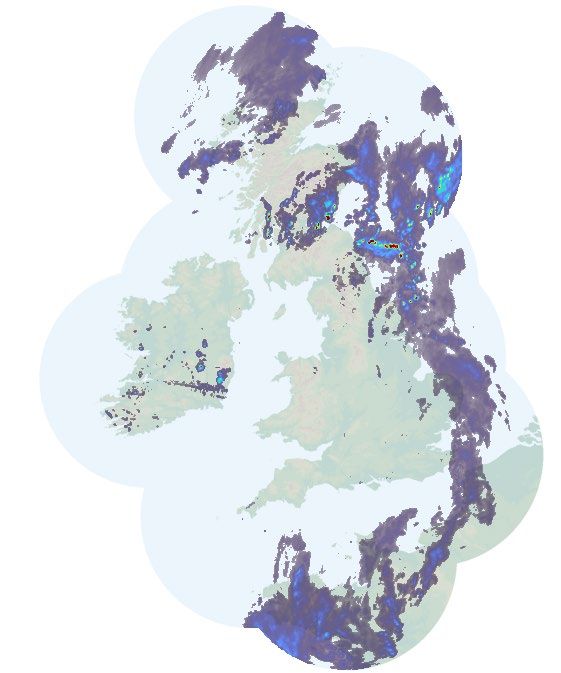
a                                         PySTEPS                  Axial attention                    DGMR
                                                                UNet                     Axial attention mode               DGMR—recal

                                               Precipitation ≥ 1.0 mm h−1             Precipitation ≥ 4.0 mm h−1            Precipitation ≥ 8.0 mm h−1
                                0.8

                                0.6

                          CSI
                                0.4

                                0.2

                                     0
                                               20      40       60      80            20      40       60      80           20      40       60      80
                                                Prediction interval (min)              Prediction interval (min)             Prediction interval (min)

                      b                          T + 30 min                                T + 90 min                                T + 90 min
                                40                                           40                                        40

                                20                                           20                                        20
                          PSD

                                 0                                            0                                         0

                            −20                                              −20                                      −20
                                               Obs. 1 km                                 Obs. 1 km                                Obs. 1 km
                                               Obs. 8 km                                 Obs. 32 km                               Obs. 16 km
                            −40                                              −40                                      −40
                                         1,024 256   64    16   4                  1,024 256   64     16   4                1,024 256   64     16   4
                                              Wavelength (km)                           Wavelength (km)                          Wavelength (km)

Fig. 2 | Deterministic verification scores for the UK in 2019. a, CSI across                   spectral density for full-frame 2019 predictions for all models at T + 30 min
20 samples for precipitation thresholds at 1 mm h−1 (left), 4 mm h−1 (middle) and              (left) and T + 90 min (middle and right). At T + 90 min, UNet (middle) has an
8 mm h−1 (right). We also report results for the axial attention mode prediction.              effective resolution of 32 km; both axial attention (right) sample and mode
UNet generates a single deterministic prediction. b, Radially averaged power                   predictions have an effective resolution of 16 km.

size31. When measured at the grid-resolution level, DGMR, PySTEPS                                 We report the relative economic value of the ensemble prediction to
and axial attention perform similarly; we also show an axial attention                         quantitatively evaluate the benefit of probabilistic predictions using
model with improved performance obtained by rescaling its output                               a simple and widely used decision-analytic model22; see the Supple-
probabilities32 (denoted ‘axial attention temp. opt.’). As the spatial                         mentary Information for a description. Figure 4a shows that DGMR
aggregation is increased, DGMR and PySTEPS provide consistently                                provides the highest economic value relative to the baseline methods
strong performance, with DGMR performing better on maximum pre-                                (has highest peak and greater area under the curve). We use 20 member
cipitation. The axial attention model is significantly poorer for larger                       ensembles and show three accumulation levels used for weather warn-
aggregations and underperforms all other methods at scale four and                             ings by Met Éireann (the Irish Meteorological service uses warnings
above. Using alternating weeks as independent units, paired permuta-                           defined directly in mm h−1; https://www.met.ie/weather-warnings).
tion tests show that the performance differences between DGMR and                              This analysis shows the ability of the generative ensemble to capture
the axial attention temp. opt. are significant (n = 26, P < 10−3).                             uncertainty, and we show the improvement with samples in Extended
   NWP and PySTEPS methods include post-processing that is used                                Data Figs. 4 and 9, and postage stamp plots to visualize the ensemble
by default in their evaluation to improve reliability. We show a simple                        variability in Supplementary Data 1–3.
post-processing method for DGMR in Figs. 2 and 3 (denoted ‘recal’)                                Importantly, we ground this economic evaluation by directly assess-
(Methods), which further improves its skill scores over the uncalibrated                       ing decision-making value using the judgments of expert meteorolo-
approach. Post-processing improves the reliability diagrams and rank                           gists working in the 24/7 operational centre at the Met Office (the UK’s
histogram to be as or more skilful than the baseline methods (Extended                         national meteorology service). We conducted a two-phase experimen-
Data Fig. 4). We also show evaluation on other metrics, performance on                         tal study to assess expert judgements of value, involving a panel of
a data split over weeks rather than years, and evaluation recapitulating                       56 experts. In phase 1, all meteorologists were asked to provide a ranked
the inability of NWPs to make predictions at nowcasting timescales                             preference assessment on a set of nowcasts with the instruction that
(Extended Data Figs. 4–6). We show results on a US dataset in Extended                         ‘preference is based on [their] opinion of accuracy and value’. Each
Data Figs. 7–9.                                                                                meteorologist assessed a unique set of nowcasts, which, at the popu-
   Together, these results show that the generative approach verifies                          lation level, allows for uncertainty characteristics and meteorologist
competitively compared to alternatives: it outperforms (on CSI) the                            idiosyncrasies to be averaged out in reporting the statistical effect. We
incumbent STEPS nowcasting approach, provides probabilistic fore-                              randomly selected 20% of meteorologists to participate in a phase 2
casts that are more location accurate, and preserves the statistical                           retrospective recall interview33.
properties of precipitation across spatial and temporal scales without                            Operational meteorologists seek utility in forecasts for critical
blurring whereas other deep learning methods do so at the expense                              events, safety and planning guidance. Therefore, to make meaningful
of them.                                                                                       statements of operational usefulness, our evaluation assessed now-
                                                                                               casts for high-intensity events, specifically medium rain (rates above
                                                                                               5 mm h−1) and heavy rain (rates above 10 mm h−1). Meteorologists were
Forecast value evaluation                                                                      asked to rank their preferences on a sample of 20 unique nowcasts
We use both economic and cognitive analyses to show that the improved                          (from a corpus of 2,126 events, being all high-intensity events in 2019).
skill of DGMR results in improved decision-making value.                                       Data were presented in the form shown in Fig. 1b, c, showing clearly the

                                                                                                                            Nature | Vol 597 | 30 September 2021 | 675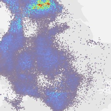
Article
                      a                                                      PySTEPS                   Axial attention                           DGMR
                                                                             UNet                      Axial attention temp. opt.                DGMR—recal

                                                             Pooling scale = 1 km                           Pooling scale = 4 km                        Pooling scale = 16 km
                                        0.100

                      Avg-pooled CRPS
                                        0.075

                                        0.050

                                        0.025

                                               0
                                                           20      40       60       80                 20      40       60       80                20      40       60       80
                                                            Prediction interval (min)                    Prediction interval (min)                   Prediction interval (min)

                         b
                                                          Pooling scale = 1 km                           Pooling scale = 4 km                       Pooling scale = 16 km
                                        0.6
                      Max-pooled CRPS

                                        0.4

                                        0.2

                                         0
                                                         20      40       60        80                 20      40       60        80               20      40       60        80
                                                          Prediction interval (min)                     Prediction interval (min)                   Prediction interval (min)

Fig. 3 | Probabilistic verification scores for the UK in 2019. Graphs show CRPS scores at the grid resolution (left), 4-km aggregations (middle) and 16-km
aggregations (right). a, Pooled CRPS using the average rain rate. b, Pooled CRPS using the maximum rain rate.

initial context at T + 0 min, the ground truth at T + 30 min, T + 60 min,                                           P < 10−4). We compute the P value assessing the binary decision whether
and T + 90 min, and nowcasts from PySTEPS, axial attention and DGMR.                                                meteorologists chose DGMR as their first choice using a permutation
The identity of the methods in each panel was anonymized and their                                                  test with 10,000 resamplings. We indicate the Clopper–Pearson CI.
order randomized. See the Methods for further details of the protocol                                               This significant meteorologist preference is important as it is strong
and of the ethics approval for human subjects research.                                                             evidence that generative nowcasting can provide meteorologists with
   The generative nowcasting approach was significantly preferred by                                                physical insight not provided by alternative methods, and provides a
meteorologists when asked to make judgments of accuracy and value of                                                grounded verification of the economic value analysis in Fig. 4a.
the nowcast, being their most preferred 89% (95% confidence interval                                                   Meteorologists were not swayed by the visual realism of the pre-
(CI) [0.86, 0.92]) of the time for the 5 mm h−1 nowcasts (Fig. 4c; P < 10−4),                                       dictions, and their responses in the subsequent structured inter-
and 90% (95% CI [0.87, 0.92]) for the 10 mm h−1 nowcasts (Fig. 4d,                                                  views showed that they approached this task by making deliberate

                                              a                                     PySTEPS                  Axial attention sample              DGMR—recal
                                                                                    UNet                     DGMR

                                                             Cumulative rain ≥ 5 mm                   Cumulative rain ≥ 10 mm                    Cumulative rain ≥ 15 mm

                                                   0.7                                                                                0.30
                                                   0.6                                     0.4                                        0.25
                                                   0.5                                     0.3                                        0.20
                                                   0.4
                                          Value

                                                                                                                                      0.15
                                                   0.3                                     0.2
                                                                                                                                      0.10
                                                   0.2
                                                                                           0.1
                                                   0.1                                                                                0.05
                                                    0                                       0                                           0
                                                         0     0.2 0.4 0.6 0.8 1.0                0     0.2 0.4 0.6 0.8 1.0                  0     0.2 0.4 0.6 0.8 1.0
                                                                 Cost/loss ratio                            Cost/loss ratio                          Cost/loss ratio

                                              b                  Most preferred from Fig. 1       c Most preferred 5 mm h−1            d Most preferred 10 mm h−1
                                              Axial attention         0.02                                   0.03                                0.02
                                                    PySTEPS           0.05                                    0.08                                0.08
                                                         DGMR                       0.93                                      0.89                                0.90

                                                                 0            0.5           1.0         0      0.25 0.50 0.75                0     0.25 0.50 0.75
                                                                     Proportion selected                     Proportion selected                 Proportion selected

Fig. 4 | DGMR provides greater decision-making value when assessed using                                            rankings for medium rain (5 mm h−1) cases. d, Meteorologist rankings for heavy
both economic and cognitive analyses. a, Relative economic value analysis                                           rain (10 mm h−1) cases. Horizontal bars show the percentage of meteorologists
across 20 samples for three 90-min rainfall accumulations, using 4-km                                               who chose each method as their first choice. Whisker lines show the Clopper–
aggregations. UNet generates a single deterministic prediction.                                                     Pearson 95% confidence interval. Meteorologists significantly preferred
b, Meteorologist preferences for the case study in Fig. 1. c, Meteorologist                                         DGMR to alternatives (n = 56, P < 10 −4).

676 | Nature | Vol 597 | 30 September 2021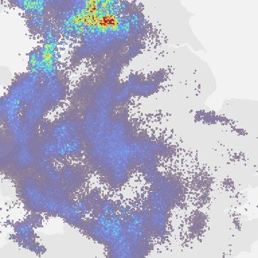
judgements of accuracy, location, extent, motion and rainfall inten-                               5.    Ayzel, G., Scheffer, T. & Heistermann, M. Rainnet v1.0: a convolutional neural network for
                                                                                                         radar-based precipitation nowcasting. Geosci. Mod. Dev. 13, 2631–2644 (2020).
sity, and reasonable trade-offs between these factors (Supplemen-                                  6.    Shi, X. et al. Deep learning for precipitation nowcasting: a benchmark and a new
tary Information, section C.6). In the phase 2 interviews, PySTEPS was                                   model. In Advances in Neural Information Processing Systems vol. 30, 5617–5627
described as “being too developmental which would be misleading”,                                        (NeurIPS, 2017).
                                                                                                   7.    Toth, Z. & Kalnay, E. Ensemble forecasting at NCEP and the breeding method. Mon.
that is, as having many “positional errors” and “much higher intensity                                   Weather Rev. 125, 3297–3319 (1997).
compared with reality”. The axial attention model was described as “too                            8.    Pierce, C., Seed, A., Ballard, S., Simonin, D. & Li, Z. In Doppler Radar Observations:
bland”, that is, as being “blocky” and “unrealistic”, but had “good spatial                              Weather Radar, Wind Profiler, Ionospheric Radar, and Other Advanced Applications (eds
                                                                                                         Bech, J. & Chau, J. L.) 97–142 (IntechOpen, 2012).
extent”. Meteorologists described DGMR as having the “best envelope”,                              9.    Sun, J. Convective-scale assimilation of radar data: progress and challenges. Quart.
“representing the risk best”, as having “much higher detail compared                                     J. Roy. Meteorol. Soc. 131, 3439–3463 (2005).
to what [expert meteorologists] are used to at the moment”, and as                                 10.   Buehner, M. & Jacques, D. Non-Gaussian deterministic assimilation of radar-derived
                                                                                                         precipitation accumulations. Mon. Weather Rev. 148, 783–808 (2020).
capturing “both the size of convection cells and intensity the best”. In                           11.   Harrison, D. et al. The evolution of the Met Office radar data quality control and product
the cases where meteorologists chose PySTEPS or the axial attention                                      generation system: Radarnet. In AMS Conference on Radar Meteorology 14–18 (AMS,
as their first choice, they pointed out that DGMR showed decay in the                                    2015).
                                                                                                   12.   Germann, U. & Zawadzki, I. Scale dependence of the predictability of precipitation from
intensity for heavy rainfall at T + 90 min and had difficulty predicting                                 continental radar images. Part II: probability forecasts. J. Appl. Meteorol. 43, 74–89 (2004).
isolated showers, which are important future improvements for the                                  13.   Imhoff, R., Brauer, C., Overeem, A., Weerts, A. & Uijlenhoet, R. Spatial and temporal
method. See the Supplementary Information for further reports from                                       evaluation of radar rainfall nowcasting techniques on 1,533 events. Water Resour. Res. 56,
                                                                                                         e2019WR026723 (2020).
this phase of the meteorologist assessment.                                                        14.   Lebedev, V. et al. Precipitation nowcasting with satellite imagery. In International
                                                                                                         Conference on Knowledge Discovery & Data Mining 2680–2688 (ACM, 2019).
                                                                                                   15.   Agrawal, S. et al. Machine learning for precipitation nowcasting from radar images.
                                                                                                         Preprint at https://arxiv.org/abs/1912.12132 (2019).
Conclusion                                                                                         16.   Trebing, K., Stańczyk, T. & Mehrkanoon, S. SmaAt-UNet: precipitation nowcasting using a
Skilful nowcasting is a long-standing problem of importance for much                                     small attention-UNet architecture. Pattern Recog. Lett. 145, 178–186 (2021).
of weather-dependent decision-making. Our approach using deep                                      17.   Xingjian, S. et al. Convolutional LSTM network: a machine learning approach for
                                                                                                         precipitation nowcasting. In Advances in Neural Information Processing Systems vol. 28,
generative models directly tackles this important problem, improves                                      802–810 (NeurIPS, 2015).
on existing solutions and provides the insight needed for real-world                               18.   Foresti, L., Sideris, I. V., Nerini, D., Beusch, L. & Germann, U. Using a 10-year radar archive
                                                                                                         for nowcasting precipitation growth and decay: a probabilistic machine learning
decision-makers. We showed—using statistical, economic and cogni-
                                                                                                         approach. Weather Forecast. 34, 1547–1569 (2019).
tive measures—that our approach to generative nowcasting provides                                  19.   Sønderby, C. K. et al. MetNet: a neural weather model for precipitation forecasting.
improved forecast quality, forecast consistency and forecast value,                                      Preprint at https://arxiv.org/abs/2003.12140 (2020).
                                                                                                   20.   Jolliffe, I. T. & Stephenson, D. B. Forecast Verification: A Practitioner’s Guide in
providing fast and accurate short-term predictions at lead times where
                                                                                                         Atmospheric Science (John Wiley & Sons, 2012).
existing methods struggle.                                                                         21.   Palmer, T. & Räisänen, J. Quantifying the risk of extreme seasonal precipitation events in a
   Yet, there remain challenges for our approach to probabilistic now-                                   changing climate. Nature 415, 512–514 (2002).
                                                                                                   22.   Richardson, D. S. Skill and relative economic value of the ECMWF ensemble prediction
casting. As the meteorologist assessment demonstrated, our genera-
                                                                                                         system. Quart. J. Roy. Meteorol. Soc. 126, 649–667 (2000).
tive method provides skilful predictions compared to other solutions,                              23.   Goodfellow, I. et al. Generative adversarial nets. In Advances in Neural Information
but the prediction of heavy precipitation at long lead times remains                                     Processing Systems vol. 27, 2672–2680 (NeurIPS, 2014).
                                                                                                   24.   Brock, A., Donahue, J. & Simonyan, K. Large scale GAN training for high fidelity
difficult for all approaches. Critically, our work reveals that standard
                                                                                                         natural image synthesis. In International Conference on Learning Representations
verification metrics and expert judgments are not mutually indica-                                       (ICLR, 2019).
tive of value, highlighting the need for newer quantitative measure-                               25.   Mirza, M. & Osindero, S. Conditional generative adversarial nets. Preprint at https://arxiv.
                                                                                                         org/abs/1411.1784 (2014).
ments that are better aligned with operational utility when evaluating                             26.   Clark, A., Donahue, J. & Simonyan, K. Adversarial video generation on complex datasets.
models with few inductive biases and high capacity. Whereas existing                                     Preprint at https://arxiv.org/abs/1907.06571 (2019).
practice focuses on quantitative improvements without concern for                                  27.   Schaefer, J. T. The critical success index as an indicator of warning skill. Weather Forecast.
                                                                                                         5, 570–575 (1990).
operational utility, we hope this work will serve as a foundation for new                          28.   Harris, D., Foufoula-Georgiou, E., Droegemeier, K. K. & Levit, J. J. Multiscale statistical
data, code and verification methods—as well as the greater integration                                   properties of a high-resolution precipitation forecast. J. Hydrol. 2, 406–418 (2001).
of machine learning and environmental science in forecasting larger                                29.   Sinclair, S. & Pegram, G. Empirical mode decomposition in 2-D space and time: a tool for
                                                                                                         space-time rainfall analysis and nowcasting. Hydrol. Earth Sys. Sci. 9, 127–137 (2005).
sets of environmental variables—that makes it possible to both provide                             30.   Gneiting, T. & Raftery, A. E. Strictly proper scoring rules, prediction, and estimation. J. Am.
competitive verification and operational utility.                                                        Stat. Assoc. 102, 359–378 (2007).
                                                                                                   31.   Gilleland, E., Ahijevych, D., Brown, B. G., Casati, B. & Ebert, E. E. Intercomparison of spatial
                                                                                                         forecast verification methods. Weather Forecast. 24, 1416–1430 (2009).
                                                                                                   32.   Guo, C., Pleiss, G., Sun, Y. & Weinberger, K. Q. On calibration of modern neural
Online content                                                                                           networks. In International Conference on Machine Learning vol. 34, 1321–1330
Any methods, additional references, Nature Research reporting sum-                                       (ICLR, 2017).
                                                                                                   33.   Crandall, B. W. & Hoffman, R. R. In The Oxford Handbook of Cognitive Engineering
maries, source data, extended data, supplementary information,                                           (ed. Lee, J. D.) 229–239 (Oxford Univ. Press, 2013).
acknowledgements, peer review information; details of author con-
                                                                                                   Publisher’s note Springer Nature remains neutral with regard to jurisdictional claims in
tributions and competing interests; and statements of data and code                                published maps and institutional affiliations.
availability are available at https://doi.org/10.1038/s41586-021-03854-z.
                                                                                                                      Open Access This article is licensed under a Creative Commons Attribution
                                                                                                                      4.0 International License, which permits use, sharing, adaptation, distribution
1.   Wilson, J. W., Feng, Y., Chen, M. & Roberts, R. D. Nowcasting challenges during the Beijing                      and reproduction in any medium or format, as long as you give appropriate
     Olympics: Successes, failures, and implications for future nowcasting systems. Weather        credit to the original author(s) and the source, provide a link to the Creative Commons license,
     Forecast. 25, 1691–1714 (2010).                                                               and indicate if changes were made. The images or other third party material in this article are
2.   Schmid, F., Wang, Y. & Harou, A. Guidelines for Nowcasting Techniques vol. 1198 (World        included in the article’s Creative Commons license, unless indicated otherwise in a credit line
     Meteorological Organization, 2017).                                                           to the material. If material is not included in the article’s Creative Commons license and your
3.   Bowler, N. E., Pierce, C. E. & Seed, A. W. STEPS: a probabilistic precipitation forecasting   intended use is not permitted by statutory regulation or exceeds the permitted use, you will
     scheme which merges an extrapolation nowcast with downscaled NWP. Quart. J. Roy.              need to obtain permission directly from the copyright holder. To view a copy of this license,
     Meteorol. Soc. 132, 2127–2155 (2006).                                                         visit http://creativecommons.org/licenses/by/4.0/.
4.   Pulkkinen, S. et al. PySTEPS: an open-source Python library for probabilistic precipitation
     nowcasting (v1. 0). Geosci. Mod. Dev. 12, 4185–4219 (2019).                                   © The Author(s) 2021

                                                                                                                                       Nature | Vol 597 | 30 September 2021 | 677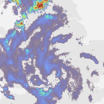
Article
Methods
                                                                              Architecture design. The nowcasting model is a generator that is
We provide additional details of the data, models and evaluation here,        trained using two discriminators and an additional regularization term.
with references to extended data that add to the results provided in          Extended Data Fig. 1 shows a detailed schematic of the generative model
the main text.                                                                and the discriminators. More precise descriptions of these architec-
                                                                              tures are given in Supplement B and corresponds to the code descrip-
Datasets                                                                      tion; pseudocode is also available in the Supplementary Information.
A dataset of radar for the UK was used for all the experiments in the            The generator in Fig. 1a comprises the conditioning stack which
main text. Additional quantitative results on a US dataset are available      processes past four radar fields that is used as context. Making effective
in Supplementary Information section A.                                       use of such context is typically a challenge for conditional generative
                                                                              models, and this stack structure allows information from the context
UK dataset                                                                    data to be used at multiple resolutions, and is used in other competi-
To train and evaluate nowcasting models over the UK, we use a collec-         tive video GAN models, for example, in ref. 26. This stack produces a
tion of radar composites from the Met Office RadarNet4 network. This          context representation that is used as an input to the sampler. A latent
network comprises more than 15 operational, proprietary C-band dual           conditioning stack takes samples from N(0, 1) Gaussian distribution,
polarization radars covering 99% of the UK (see figure 1 in ref. 34). We      and reshapes into a second latent representation. The sampler is a
refer to ref. 11 for details about how radar reflectivity is post-processed   recurrent network formed with convolutional gated recurrent units
to obtain the two-dimensional radar composite field, which includes           (GRUs) that uses the context and latent representations as inputs. The
orographic enhancement and mean field adjustment using rain gauges.           sampler makes predictions of 18 future radar fields (the next 90 min).
Each grid cell in the 1,536 × 1,280 composite represents the surface-level    This architecture is both memory efficient and has had success in other
precipitation rate (in mm h−1) over a 1 km × 1 km region in the OSGB36        forecasting applications. We also made comparisons with longer con-
coordinate system. If a precipitation rate is missing (for example,           text using the past 6 or 8 frames, but this did not result in appreciable
because the location is not covered by any radar, or if a radar is out of     improvements.
order), the corresponding grid cell is assigned a negative value which           Two discriminators in Fig. 1b are used to allow for adversarial learn-
is used to mask the grid cell at training and evaluation time. The radar      ing in space and time. The spatial and temporal discriminator share
composites are quantized in increments of 1/32 mm h−1.                        the same structure, except that the temporal discriminator uses 3D
   We use radar collected every five minutes between 1 January 2016 and       convolutions to account for the time dimension. Only 8 out of 18 lead
31 December 2019. We use the following data splits for model develop-         times are used in the spatial discriminator, and a random 128 × 128
ment. Fields from the first day of each month from 2016 to 2018 are           crop used for the temporal discriminator. These choices allow the
assigned to the validation set. All other days from 2016 to 2018 are          models to fit within memory. We include a spatial attention block in the
assigned to the training set. Finally, data from 2019 are used for the        latent conditioning stack since it allows the model to be more robust
test set, preventing data leakage and testing for out of distribution         across different types of regions and events, and provides an implicit
generalization. For further experiments testing in-distribution per-          regularization to prevent overfitting, particularly for the US dataset.
formance using a different data split, see Supplementary Information             Both the generator and discriminators use spectrally normalized
section C.                                                                    convolutions throughout, similar to ref. 35, since this is widely estab-
                                                                              lished to improve optimization. During model development, we initially
Training set preparation                                                      found that including a batch normalization layer (without variance
Most radar composites contain little to no rain. Supplementary Table 2        scaling) prior to the linear layer of the two discriminators improved
shows that approximately 89% of grid cells contain no rain in the UK.         training stability. The results presented use batch normalization, but
Medium to heavy precipitation (using rain rate above 4 mm h−1) com-           we later were able to obtain nearly identical quantitative and qualita-
prises fewer than 0.4% of grid cells in the dataset. To account for this      tive results without it.
imbalanced distribution, the dataset is rebalanced to include more
data with heavier precipitation radar observations, which allows the          Objective function. The generator is trained with losses from the two
models to learn useful precipitation predictions.                             discriminators and a grid cell regularization term (denoted LR (θ) ). The
   Each example in the dataset is a sequence of 24 radar observations         spatial discriminator Dϕ has parameters ϕ, the temporal discriminator
of size 1,536 × 1,280, representing two continuous hours of data. The         Tψ has parameters ψ, and the generator Gθ has parameters θ. We indicate
maximum rain rate is capped at 128 mm h−1, and sequences that are             the concatenation of two fields using the notation {X; G} . The genera-
missing one or more radar observations are removed. 256 × 256 crops           tor objective that is maximized is
are extracted and an importance sampling scheme is used to reduce
the number of examples containing little precipitation. We describe                       L G(θ) = E X 1: M + N[EZ[D(Gθ(Z ; X 1:M ))
                                                                                                                                                               (2)
this importance sampling and the parameters used in Supplementary                                    + T ({X 1:M ; Gθ(Z ; X 1:M )})] − λ LR(θ)];
Information section A.1. After subsampling and removing entirely
masked examples, the number of examples in the training set is roughly
1.5 million.                                                                                  1
                                                                                   LR (θ) =
                                                                                             HWN                                                               (3)
Model details and baselines                                                               ||(EZ [Gθ (Z ; X 1:M )] − X M +1:M + N ]) ⊙ w (X M +1:M + N )||1 .
Here, we describe the proposed method and the three baselines to
which we compare performance. When applicable, we describe both               We use Monte Carlo estimates for expectations over the latent Z in
the architectures of the models and the training methods. There is a          equations (2) and (3). These are calculated using six samples per input
wealth of prior work, and we survey them as additional background             X1:M, which comprises M = 4 radar observations. The grid cell regularizer
in Supplementary Information section E.                                       ensures that the mean prediction remains close to the ground truth,
                                                                              and is averaged across all grid cells along the height H, width W and
DGMR                                                                          lead-time N axes. It is weighted towards heavier rainfall targets using
A high-level description of the model was given in the main text and          the function w(y) = max(y + 1, 24), which operate element-wise for
in Fig. 1a, and we provide some insight into the design decisions here.       input vectors, and is clipped at 24 for robustness to spuriously large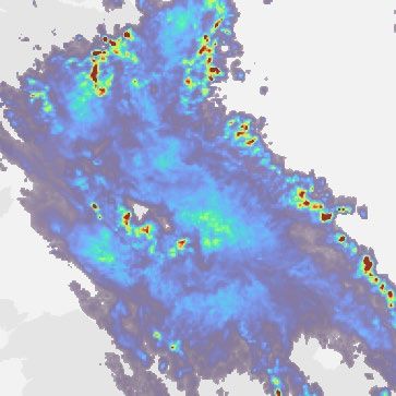
values in the radar. The GAN spatial discriminator loss LD (ϕ) and tem-        of the latent representation followed by spatial down-sampling by a
poral discriminator loss L T (ψ) are minimized with respect to param-          factor of two. The representation with the highest resolution has 32
eters ϕ and ψ, respectively; ReLU (x) = max(0, x). The discriminator           channels which increases up to 1,024 channels.
losses use a hinge loss formulation26:                                            Similar to ref. 6, we use a loss weighted by precipitation intensity.
                                                                               Rather than weighting by precipitation bins, however, we reweight
             LD(φ) = E X 1: M + N, Z[ReLU(1 − Dφ(X M +1:M + N ))               the loss directly by the precipitation to improve results on thresholds
                                                                        (4)    outside of the bins specified by ref. 6. Additionally, we truncate the
                         + ReLU(1 + Dφ(G(Z ; X 1:M )))].
                                                                               maximum weight to 24 mm h−1 as an error in reflectivity of observations
                                                                               leads to larger error in the precipitation values. We also found that
             L T(ψ) = E X 1: M + N, Z[ReLU(1 − Tψ(X 1:M + N ))                 including a mean squared error loss made predictions more sensitive
                                                                        (5)    to radar artefacts; as a result, the model is only trained with precipita-
                       +ReLU(1 + Tψ({X 1:M ; G(Z ; X 1:M )}))].
                                                                               tion weighted mean average error loss.
                                                                                  The model is trained with batch size eight for 1 × 10⁶ steps, with
Evaluation. During evaluation, the generator architecture is the same,         learning rate 2 × 10⁻⁴ with weight decay, using the Adam optimizer
but unless otherwise noted, full radar observations of size 1,536 × 1,280,     with default exponential rates. We select a model using early stop-
and latent variables with height and width 1/32 of the radar observation       ping on the average area under the precision–recall curve on the
size (48 × 40 × 8 of independent draws from a normal distribution),            validation set. The UNet baselines are trained with 4 frames of size
are used as inputs to the conditioning stack and latent conditioning           256 × 256 as context.
stack, respectively. In particular, the latent conditioning stack allows
for spatiotemporally consistent predictions for much larger regions            Axial attention baseline
than those on which the generator is trained.                                  As a second strong deep learning-based baseline, we adapt the MetNet
   For operational purposes and decision-making, the most impor-               model19, which is a combination of a convolutional long short-term
tant aspect of a probabilistic prediction is its resolution36. Specific        memory (LSTM) encoder17 and an axial attention decoder39, for
applications will require different requirements on reliability that can       radar-only nowcasting. MetNet was demonstrated to achieve strong
often be addressed by post-processing and calibration. We develop              results on short-term (up to 8 h) low precipitation forecasting using
one possible post-processing approach to improve the reliability of            radar and satellite data of the continental USA, making per-grid-cell
the generative nowcasts. At prediction time, the latent variables are          probabilistic predictions and factorizing spatial dependencies using
samples from a Gaussian distribution with standard deviation 2 (rather         alternating layers of axial attention.
than 1), relying on empirical insights on maintaining resolution while            We modified the axial attention encoder–decoder model to use radar
increasing sample diversity in generative models24,37. In addition, for        observations only, as well as to cover the spatial and temporal extent of
each realization we apply a stochastic perturbation to the input radar         data in this study. We rescaled the targets of the model to improve its
by multiplying a single constant drawn from a unit-mean gamma dis-             performance on forecasts of heavy precipitation events. After evalu-
tribution G(α = 5, β = 5) to the entire input radar field. Extended Data       ation on both UK and US data, we observed that additional satellite or
Figures 4 (UK) and 9 (US) shows how the post-processing improves               topographical data as well as the spatiotemporal embeddings did not
the reliability diagram and rank histogram compared to the uncor-              provide statistically significant CSI improvement. An extended descrip-
rected approach.                                                               tion of the model and its adaptations is provided in Supplementary
                                                                               Information section D.
Training. The model is trained for 5 × 10⁵ generator steps, with two dis-         The only prediction method described in ref. 19 is the per-grid-cell
criminator steps per generator step. The learning rate for the generator       distributional mode, and this is considered the default method for
is 5 × 10⁻⁵, and is 2 × 10⁻⁴ for the discriminator and uses Adam optimizer38   comparison. To ensure the strongest baseline model, we also evaluated
with β1 = 0.0 and β2 = 0.999. The scaling parameter for the grid cell regu-    other prediction approaches. We assessed using independent samples
larization is set to λ = 20, as this produced the best continuous ranked       from the per-grid-cell marginal distributions, but this was not better
probability score results on the validation set. We train on 16 tensor         than using the mode when assessed quantitatively and qualitatively.
processing unit cores (https://cloud.google.com/tpu) for one week on           We also combined the marginal distributions with a Gaussian process
random crops of the training dataset of size 256 × 256 measurements            copula, in order to incorporate spatiotemporal correlation similar
using a batch size of 16 per training step. The Supplementary Informa-         to the stochastically perturbed parametrization tendencies (SPPT)
tion contains additional comparisons showing the contributions of              scheme of ref. 40. We used kernels and correlation scales chosen to
the different loss components to overall performance. We evaluated             minimize spatiotemporally pooled CRPS metrics. The best perform-
the speed of sampling by comparing speed on both CPU (10 core AMD              ing was the product of a Gaussian kernel with 25 km spatial correla-
EPYC) and GPU (NVIDIA V100) hardware. We generate ten samples and              tion scale, and an AR(1) kernel with 60 min temporal correlation scale.
report the median time: for CPU the median time per sample was 25.7 s,         Results, however, were not highly sensitive to these choices. All set-
and 1.3 s for the GPU.                                                         tings resulted in samples that were not physically plausible, due to the
                                                                               stationary and unconditional correlation structure. These samples
UNet baseline                                                                  were also not favoured by external experts. Hence, we use the mode
We use a UNet encoder–decoder model as strong baseline similarly               prediction throughout.
to how it was used in related studies5,15, but we make architectural and
loss function changes that improve its performance at longer lead              PySTEPS baseline
times and heavier precipitation. First, we replace all convolutional           We use the PySTEPS implementation from ref. 4 using the default con-
layers with residual blocks, as the latter provided a small but consist-       figuration available at https://github.com/pySTEPS/pysteps. Refs. 3,4
ent improvement across all prediction thresholds. Second, rather than          provide more details of this approach. In our evaluation, unlike other
predicting only a single output and using autoregressive sampling              models evaluated that use inputs of size 256 × 256, PySTEPS is given
during evaluation, the model predicts all frames in a single forward           the advantage of being fed inputs of size 512 × 512, which was found
pass. This somewhat mitigates the excessive blurring found in ref. 5 and       to improve its performance. PySTEPS includes post-processing using
improves results on quantitative evaluation. Our architecture consists         probability matching to recalibrate its predictions and these are used
of six residual blocks, where each block doubles the number of channels        in all results.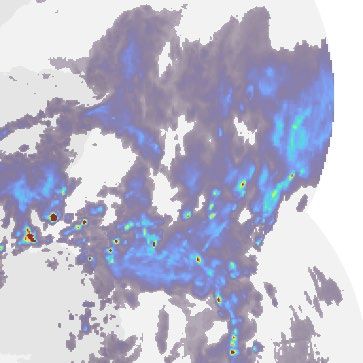
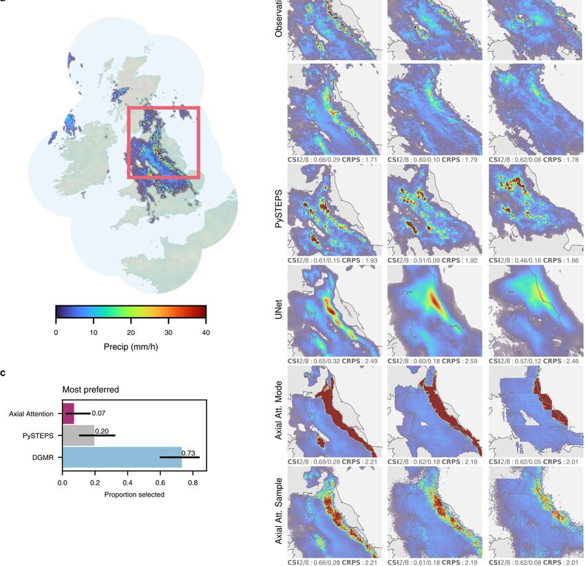
Article
                                                                             meteorologists as part of the evaluative study, and in both cases, mete-
Performance evaluation                                                       orologists significantly preferred the generative approach (n = 56,
We evaluate our model and baselines using commonly used quantita-            P < 10−4) to competing methods. For the high-intensity precipitation
tive verification measures, as well as qualitatively using a cognitive       front in Extended Data Fig. 2, meteorologists ranked first the genera-
assessment task with expert meteorologists. Unless otherwise noted,          tive approach in 73% of cases. Meteorologists reported that DGMR has
models are trained on years 2016–2018 and evaluated on 2019 (that is,        “decent accuracy with both the shape and intensity of the feature … but
a yearly split).                                                             loses most of the signal for embedded convection by T + 90”. PySTEPS
                                                                             is “too extensive with convective cells and lacks the organisation seen
Expert meteorologist study                                                   in the observations”, and the axial attention model as “highlighting the
The expert meteorologist study described is a two-phase protocol             worst areas” but “looks wrong”.
consisting of a ranked comparison task followed by a retrospective              For the cyclonic circulation in Extended Data Fig. 3, meteorologists
recall interview. The study was submitted for ethical assessment to an       ranked first the generative approach in 73% of cases. Meteorologists
independent ethics committee and received favourable review. Key ele-        reported that it was difficult to judge this case between DGMR and
ments of the protocol involved consent forms that clearly explained the      PySTEPS. When making their judgment, they chose DGMR since it has
task and time commitment, clear messaging on the ability to withdraw         “best fit and rates overall”. DGMR “captures the extent of precipitation
from the study at any point, and that the study was not an assessment        overall [in the] area, though slightly overdoes rain coverage between
of the meteorologist’s skills and would not affect their employment          bands”, whereas PySTEPS “looks less spatially accurate as time goes on”.
and role in any way. Meteorologists were not paid for participation,         The axial attention model “highlights the area of heaviest rain although
since involvement in these types of studies is considered part of the        its structure is unrealistic and too binary”. We provide additional quotes
broader role of the meteorologist. The study was anonymized, and             in Supplementary Information section C.6.
only the study lead had access to the assignment of experimental IDs.
The study was restricted to meteorologists in guidance-related roles,        Quantitative evaluation
that is, meteorologists whose role is to interpret weather forecasts, syn-   We evaluate all models using established metrics20: CSI, CRPS, Pearson
thesize forecasts and provide interpretations, warnings and watches.         correlation coefficient, the relative economic value22,41,42, and radially
Fifty-six meteorologists agreed to participate in the study.                 averaged PSD. These are described in Supplementary Information
   Phase 1 of the study, the rating assessment, involved each meteorolo-     section F.
gist receiving a unique form as part of their experimental evaluation.          To make evaluation computationally feasible, for all metrics except
The axial attention mode prediction is used in the assessment, and           PSD, we evaluate the models on a subsampled test set, consisting of
this was selected as the most appropriate prediction during the pilot        512 × 512 crops drawn from the full radar images. We use an importance
assessment of the protocol by the chief meteorologist. The phase 1           sampling scheme (described in Supplementary Information section
evaluation comprised an initial practice phase of three judgments for        A.1) to ensure that this subsampling does not unduly compromise
meteorologists to understand how to use the form and assign ratings,         the statistical efficiency of our estimators of the evaluation metrics.
followed by an experimental phase that involved 20 trials that were dif-     The subsampling reduces the size of the test set to 66,851 and Sup-
ferent for every meteorologist, and a final case study phase in which all    plementary Information section C.3 shows that results obtained when
meteorologists rated the same three scenarios (the scenarios in Fig. 1a,     evaluating CSI are not different when using the dataset with or without
and Extended Data Figs. 2 and 3); these three events were chosen by          subsampling. All models except PySTEPS are given the centre 256 × 256
the chief meteorologist—who is independent of the research team and          crop as input. PySTEPS is given the entire 512 × 512 crop as input as this
also did not take part in the study—as difficult events that would expose    improves its performance. The predictions are evaluated on the centre
challenges for the nowcasting approaches we compare. Ten meteorolo-          64 × 64 grid cells, ensuring that models are not unfairly penalized by
gists participated in the subsequent retrospective recall interview. This    boundary effects. Our statistical significance tests use every other week
interview involved an in-person interview in which experts were asked        of data in the test set (leaving n = 26 weeks) as independent units. We
to explain the reasoning for their assigned rating and what aspects          test the null hypothesis that performance metrics are equal for the two
informed their decision-making. These interviews all used the same           models, against the two-sided alternative, using a paired permutation
script for consistency, and these sessions were recorded with audio          test43 with 106 permutations.
only. Once all the audio was transcribed, the recordings were deleted.          Extended Data Figure 4 shows additional probabilistic metrics that
   The 20 trials of the experimental phase were split into two parts, each   measure the calibration of the evaluated methods. This figure shows
containing ten trials. The first ten trials comprised medium rain events     a comparison of the relative economic value of the probabilistic meth-
(rainfall greater than 5 mm h−1) and the second 10 trials comprised heavy    ods, showing DGMR providing the best value. We also show how the
rain events (rainfall greater than 10 mm h−1). 141 days from 2019 were       uncertainty captured by the ensemble increases as the number of sam-
chosen by the chief meteorologist as having medium-to-heavy precipi-         ples used is increased from 1 to 20.
tation events. From these dates, radar fields were chosen algorithmi-           Extended Data Figure 5 compares the performance to that of an NWP,
cally according to the following procedure. First, we excluded from the      using the UKV deterministic forecast44, showing that NWPs are not
crop selection procedure the 192 km that forms the image margins of          competitive in this regime. See Supplementary Information section
each side of the radar field. Then, the crop over 256 km regions, contain-   C.2 for further details of the NWP evaluation.
ing the maximum fraction of grid cells above the given threshold, 5 or          To verify other generalization characteristics of our approach—as an
10 mm h−1, was selected from the radar image. If there was no precipita-     alternative to the yearly data split that uses training data of 2016–2018 and
tion in the frame above the given threshold, the selected crop was the       tests on 2019—we also use a weekly split: where the training, validation and
one with the maximum average intensity. We use predictions without           test sets comprise Thursday through Monday, Tuesday, and Wednesday,
post-processing in the study. Each meteorologist assessed a unique           respectively. The sizes of the training and test datasets are 1.48 million and
set of predictions, which allows us to average over the uncertainty in       36,106, respectively. Extended Data Figure 6 shows the same competitive
predictions and individual preference to show statistical effect.            verification performance of DGMR in this generalization test.
   Extended Data Figure 2 shows a high-intensity precipitation front            To further assess the generalization of our method, we evaluate on a sec-
with decay and Extended Data Fig. 3 shows a cyclonic circulation event       ond dataset from the USA using the multi-radar multi-sensitivity (MRMS)
(low-pressure area), both of which are difficult for current deep learn-     dataset, which consists of radar composites for years 2017–201945.
ing models to predict. These two cases were also assessed by all expert      We use two years for training and one year for testing, and even with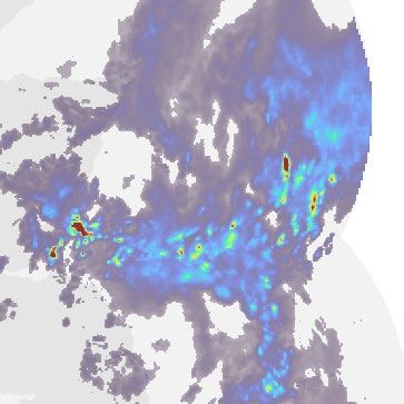
You can also read