Share My Space Multi-telescope Observation Stations Performance Assessment
←
→
Page content transcription
If your browser does not render page correctly, please read the page content below
Share My Space Multi-telescope Observation Stations
                         Performance Assessment

                                  A. Petit, R. Lucken, H. Tarrieu, D. Giolito
                      Share My Space, 32 Boulevard du Port 95032 Cergy-Pontoise, France
                                 Contact: romain.lucken@sharemyspace.space
                                                 C. Cavadore
                       Alcor System 326 Chemin d’Albigneux, 42570 St Héand, FRANCE

                                             T. Lépine
   Institut d’Optique Graduate School and Univ-Lyon, Laboratoire Hubert Curien, UMR CNRS
                    5516, 18 rue Benoı̂t Lauras, 42000 Saint-Etienne, FRANCE

                                                                August 23 2021

                                                                  ABSTRACT

Detecting and cataloging small objects in Earth orbits is a growing challenge for the space community as the space traffic is
increasing. Optical systems have a major role to play in order to tackle this challenge, with the ability to detect objects on all types
of orbits. The aim of this paper is to evaluate the potential of selected optical technologies for cataloging objects in LEO. The
detection capabilities of individual telescopes is estimated from theory and compared to observations performed with the telescopes
operated by Share My Space and analyzed with the StreakDet software. The core concept of the multi-telescope stations is a conic
fence of optical detection. The detection of a statistical population of 83 000 objects propagated over one month is simulated in
various observation network configurations. It is shown that 15 000 LEO objects larger than 3 cm can be cataloged with off-the-shelf
telescope components, and up to 53 000 with a new optical system.

                                                           1.    INTRODUCTION

The increase in space traffic in the past 5 years questions the ability of the space community to ensure the safety of
space vehicles. Ground infrastructures for space surveillance are key technologies to monitor the traffic in a compre-
hensive and timely fashion. However, cataloging objects smaller than 10 cm in size remains a challenge. The problem
is particularly acute in crowded low Earth orbits (LEO) regions were the density of satellites and space debris is high
and the relative velocities are large.
The Space Fence is a phased-array radar designed to monitor space objects below the altitude of 2,000 km. It has cost
about 3 billion dollars to the US Government [1] and allowed to detect objects down to 5 cm in size. Nevertheless,
the purpose of this facility is primarily military supremacy and the contribution to the public space object catalog has
been minor so far1 . Private companies have also started to offer Space Situational Awareness (SSA) services to the
community in the same period [2]. The solution put forward by Share My Space is purely based on passive optical
observations. While optical observation of geostationary Earth orbit (GEO) satellites has been performed routinely
within various organizations that include the United States Space Surveillance Network (US SSN) and the French
Tarot network for instance, optical observations of LEO objects is not done systematically.
Optical observation is the most affordable way to monitor space from Earth. Telescope systems are usually made of
one or multiple mirrors, sometimes combined with a set of lenses. An optical observation system for SSA is however
not limited to the optical tube only. The mount, the digital camera, as well as the GPS receiver, are critical elements
that should be correctly sized and assembled to yield an efficient system. A full observation station also includes
a motorized dome and a weather station. The infrastructure can be controlled from remote locations with a set of
   1 As   of July 2021, only between 300 and 400 objects coming from the Space Fence are tracked and cataloged on space-track.org.

                   Copyright © 2021 Advanced Maui Optical and Space Surveillance Technologies Conference (AMOS) – www.amostech.com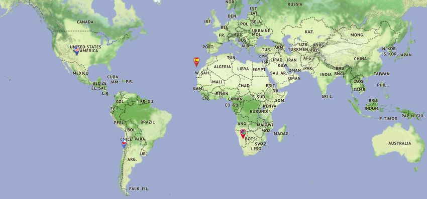
AMOS Tech                                                                                                                         2021
software programs and drivers for each of the components. Wide-field telescopes are particularly relevant for LEO
object observation, as shown by Zimmer et al. (2015) [3]. Optical observations of LEO objects by optical telescopes
used to be difficult because of the high angular velocities in the observer’s reference frame. These large angular
velocities yield a short occupation time of the objects in the field of view of a pixel of the camera, thus offering a
poor signal received. Zimmer, McGraw and Ackermann [4] introduced a solution by developing a wide field of view
telescope that is well-suited for LEO surveillance.
The first part of the paper presents a streak detection simulator. The second part is dedicated to the validation of the
performance of this simulator opposed to observation images generated by Share My Space. The last part presents the
multi-telescope observation station (MTOS) concept, with its conic detection fence, as well as the simulation results
with a full sampling of on-orbit objects larger than 3 cm over a period of 28 days.

                       2.    THE PHOTON CHAIN: FROM THE SUN TO THE DETECTOR

In this section, the basics of optical observation of on-orbit object are summarized.
2.1 Light reflection on a resident space object
Resident space objects (RSO) can be operational satellites but also defunct satellites, rocket bodies (R/B), fragments
of explosions or collisions. These objects have diverse shapes and are made of various materials. When a surface of a
RSO is illuminated by the Sun it reflects the sunlight in a specular and/or diffuse way. While in the case of specular
reflection, the reflected angle is strictly equal to the incident angle, for diffuse reflection, the reflected energy is spread
across an infinite number of directions [5]. The most common diffuse reflection law for a material is called the Lambert
surface model. A Lambert surface whose irradiance is angularly and spatially uniform. A surface seen from the side
will be seen with a smaller solid angle by the observer, and hence the total energy received will be lower. However,
only a fraction of the incident energy is reflected. This fraction is called the albedo of a surface, and noted ρ. For
space debris of unknown size and shape, the specular and diffuse reflection components can in some cases be obtained
from the comparisons with measurements performed by other sources than optics [5]. Some materials used in satellite
manufacturing can have large specular reflection components, such as multi-layer insulation (MLI) [6]. Nevertheless,
even when the surface material is known, the orientation of every single reflecting surface is practically impossible to
estimate. The common way to describe a RSO from an optical perspective is to assume that all the reflected energy is
generated diffusely and that the albedo coefficient is the ratio between the energy reflected diffusely and the incident
energy. The size and the physical properties of the RSO are difficult to assess in general. Some former studies were
dedicated to estimating the albedo coefficients of RSO and found that a value of ρ = 0.175 was a good estimate for
space debris fragments represented as spheres [7]. The problem of light reflection on a RSO hence breaks down to
the well-known problem of a Lambert sphere [8]. For completeness and to avoid erroneous referencing, we provided
the full derivation of the Lambert sphere problem in Appendix A. The main result is that the scattered irradiance Irs is
related to the Sun’s irradiance at the object location Irs,Sun,space by:

                                                               Aρ
                                                       Irs =      F(ψ)Irs,Sun,space                                                (1)
                                                               R2
where A is the surface cross section, ρ is the albedo, R is the distance between the observer and the object, ψ is the
phase angle, and F(ψ) is the phase function (see Eq. (62)). It is further assumed that all wavelengths are reflected in
the same way.
2.2 Solar spectrum through the atmosphere
The light that is reflected by the object has to propagate through the atmosphere before it can be detected by a ground
telescope. Absorption and diffusion of Sun light by the atmosphere strongly depends on the wavelength. Therefore,
the solar spectrum should be correctly modeled to get the correct amount of photons received.
The spectral radiance emitted by the Sun’s surface depends on the wavelength λ and is similar to the emission spectrum
of a black body at T = 5 750 K defined by Planck’s law:

                                                         2hc2           1
                                             Brs,Sun =                            [W/m2 /nm/sr]                                    (2)
                                                          λ5          hc
                                                                e   λ kB T   −1

                Copyright © 2021 Advanced Maui Optical and Space Surveillance Technologies Conference (AMOS) – www.amostech.com
AMOS Tech                                                                                                                        2021

where kB and h are Boltzmann’s and Planck’s constants respectively, and c the light velocity. The solid angle of the
Sun’s surface visible from the object is dΩ = cos θ dS/R2E−S = cos θ sin θ dθ dφ R2Sun /R2E−S , where RSun is the Sun’s
radius, RE−S is the distance between Earth and the Sun, dS is the elementary Sun surface area, θ and φ are here the
spherical coordinates of a surface element of the Sun. Since all the objects are close to Earth relative to the distance
between the Sun and Earth, we always use the same distance RE−S for all objects throughout this paper. By integrating
Eq. (2) over dΩ, we obtain the Sun spectral irradiance received near Earth:
                                                                                     2
                                               2hc2

                                                                π           RSun
                                      Irs,Sun = 5             hc
                                                                          ×                [W/m2 /nm]                             (3)
                                                λ                           RE−S
                                                        e   λ kB T   −1

Some wavelengths are more dampened than others because they correspond to the resonance wavelengths of some
common molecules in the atmosphere such as O2 , O3 , CO2 or H2 O. Solar data extracted from ASTM-G173 [9] are
used all through the paper. The reference data is provided with a tilt angle of 37◦ (53◦ of elevation). Figure 1(a)
shows the solar spectrum in space Irs,Sun,0 and on ground Irs,Sun,g , measured at zenith and at an elevation angle of
53◦ , compared with the irradiance obtained from the black body model (Eq. (3)). The ratio between the irradiance on
ground and in space yields the transmission coefficient of the atmosphere at an elevation of 53◦ :

                                                                     Irs,Sun,ground (λ , 53◦ )
                                                 τ(λ , 53◦ ) =                                 .                                  (4)
                                                                         Irs,Sun,space (λ )

We employ Beer-Lambert’s law to introduce the dependency of the transmission coefficient with the elevation angle e
of the observation:
                                            τ(λ , e) = τ0 (λ )1/ sin e .                                        (5)
where τ0 (λ ) is the transmittance when the Sun is at the zenith (elevation of 90◦ ).
The atmospheric optical transmission is plotted as a function of the wavelength in Figure 1(b), for three values of
elevation, 90◦ , 53◦ and 30◦ .

               Copyright © 2021 Advanced Maui Optical and Space Surveillance Technologies Conference (AMOS) – www.amostech.com
AMOS Tech                                                                                                                                     2021

                                                                      (a) Spectral irradiance from the Sun
                                                                                                             Black body at 5900 K
                                                          2.00                                               Extraterrestrial
                          Spectral irradiance [W/m2/nm]

                                                          1.75                                               On ground at zenith
                                                                                                             On ground, elevation of 53o
                                                          1.50
                                                          1.25
                                                          1.00
                                                          0.75
                                                          0.50
                                                          0.25
                                                          0.00
                                                                          400      600     800    1000 1200 1400      1600     1800    2000
                                                                                                 Wavelength [nm]
                                                                      (b) Atmospheric transmittance
                                                                1.0

                                                                0.8
                                    Atmospheric transmittance

                                                                0.6

                                                                0.4

                                                                0.2               Elevation of 90o (zenith)
                                                                                  Elevation of 53o
                                                                                  Elevation of 30o
                                                                0.0
                                                                          400      600     800 1000 1200 1400         1600     1800    2000
                                                                                                  Wavelength [nm]

Fig. 1: Spectral irradiance from the Sun and transmission through the atmosphere. (a) Comparison of the irradiance
received from the Sun in space near Earth, on ground after perpendicular transmission to the atmosphere surface
(zenith), with an elevation angle of 53◦ , and ideal irradiance from black body at 5900 K. (b) Atmospheric transmittance
computed for beams coming from the zenith, and at elevations of 53◦ and 30◦ .

               Copyright © 2021 Advanced Maui Optical and Space Surveillance Technologies Conference (AMOS) – www.amostech.com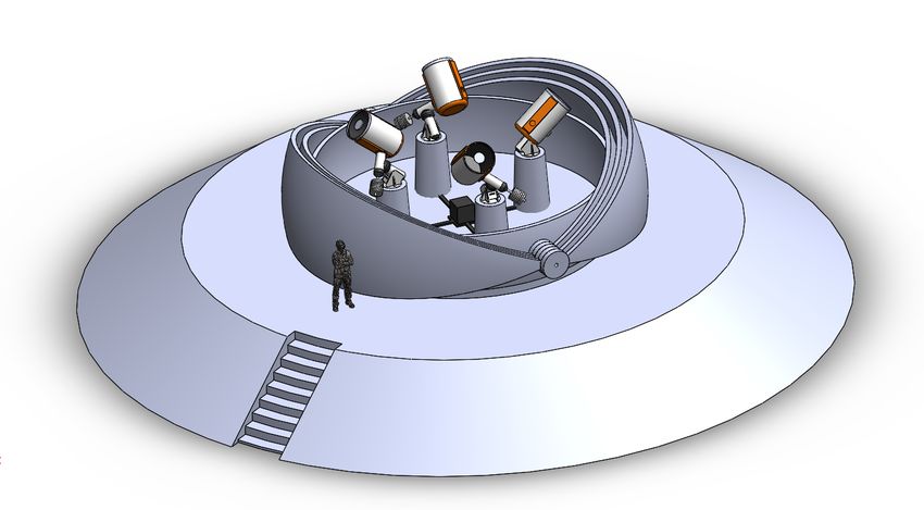
AMOS Tech                                                                                                                        2021

2.3 Signal received by the sensor
The aim of this section is to compute the amount of photons emitted by an object, based on its size and geometry, and
electrons received by the sensor.
The spectral photon irradiance collected on ground is
                                                               Irs,telescope λ
                                        Fps,telescope =                           [photons/m2 /s/nm]                              (6)
                                                                      hc
hc/λ being the photon energy. Each photon collected by the telescope from one given direction hits one pixel of
the sensor, and can generate a photo-electron in accordance with a probability equal to the quantum efficiency of the
sensor Qe that also depends on the wavelength λ . The collection surface to be taken into account is simply the telescope
aperture surface. In the optical systems considered in this paper, the angle between the light beam and the optical axis
is typically in the [−2◦ , +2◦ ] interval. Hence, the small angle approximation can be used (cos(2◦ ) = 0.9994 ≈ 1). The
spectral flux of electrons is therefore
                                                    λ QE (λ )A
                                        Ses =                  Irs,telescope           [electrons/s/nm]                           (7)
                                                        hc
where
                                                              πD2
                                                                A = (1 − ζ 2 )                                 (8)
                                                               4
is the open surface of the telescope, ζ being the telescope diameter obstruction, and D the diameter. Finally, by
integrating the electron flux for all wavelengths:
                                                  λZmax
                                                          λ QE (λ )A
                                      Se =                           Irs,telescope dλ       [electrons/s]                         (9)
                                                              hc
                                                 λmin

Furthermore, the irradiance at the telescope depends both on the diffusive reflection phenomenon described by Eq. (1)
and the transmission through the atmosphere. Thus,
                                         λZmax
                                                 Aρλ QE (λ )τ(λ )F(ψ)A
                                 Se =                                  Irs,Sun dλ               [electrons/s]                    (10)
                                                          hcR2
                                        λmin

The time spent by an object with a local angular velocity ω on a pixel with a field of view α px = l/ f , l being the size
of a pixel and f the focal length, is:
                                                             l
                                                      δt =                                                            (11)
                                                            fω
Therefore, the number of collected electrons is
                                                              λZmax
                                    AρF(ψ)A l
                               Ne =                                 λ QE (λ )τ(λ )Irs,Sun (λ ) dλ   [electrons]                  (12)
                                     hcR2 f ω
                                                             λmin

The local angular velocity ω (taking sidereal tracking into account ) can simply be determined from the velocity of
the object v and its position relative to the observation station.
                                                                        ||v − (v · u)u||
                                                                ω=                                                               (13)
                                                                               R
where u = AM/R is the unit vector pointing towards the object from the observation station. To be consistent with
previous notations, AM = ||AM|| = R.
An approximation of the local angular velocity is provided in the case where the observer is in the orbital plane in
Appendix B.

                                                                        γ(γ − cos ν)
                                                             ω=                       Ω                                          (14)
                                                                      γ 2 − 2γ cos ν
                                                                                   +1

               Copyright © 2021 Advanced Maui Optical and Space Surveillance Technologies Conference (AMOS) – www.amostech.com
AMOS Tech 2021
where γ = 1+h/RE , and ν is the true anomaly. The reader should refer to to Eq. (68) in Appendix B for the relationship
between the true anomaly and the elevation.
This analytical formula is convenient for quick estimates of the system performances.
2.4 Optical limitations and point-spread function (PSF)
Even with a perfect telescope design, some phenomena prevent the detection from being perfect. Some of these
phenomena are explained and quantified here.
2.4.1 Rayleigh criterion
Rayleigh’s criterion corresponds to the diffraction limit for a light beam that crosses a circular aperture. The central
diffraction spot, or Airy pattern, has an angular width
1.22λ
δ θdi f f raction = (15)
D
where D is the telescope aperture diameter. For a RASA 8” telescope (D = 203 mm) and for a wavelength of 1200 nm,
δ θdi f f raction = 7.2 × 10⁻⁶ rad= 1.49 arcsec. For the RASA 14” telescope, the manufacturer specifies a Rayleigh
diffraction limit of 0.39 arcsec which is slightly lower than the estimate based on a circular aperture, due to the seeing.
For a diameter of 1 m and a wavelength of 800 nm, δ θdi f f raction = 0.2 arcsec.
2.4.2 Astronomical seeing
Astronomical seeing is due to random fluctuations of the atmosphere that affect the perceived angular position of
any space object. A good seeing on clear and still nights is typically of 1 arcsecond, which is equal to δ θseeing =
4.8 × 10⁻⁶ rad. By default, we use a value of 2 arcsec for the seeing, which is a conservative value for any good
observatory location.
2.4.3 Instrument aberration
Beside the diffraction limit and the astronomical seeing, each optical instrument has it own optical aberration that
depends on the wavelength and the angular distance from the optical axis. The spot size is indicated smaller than
6.3 µm RMS by Celestron, which corresponds to δ θaberration = 1.6 arcsec.
2.4.4 Point-spread function
The point spread function represents the way the image of a singular light source is spread across pixels. It is the result
of the combination of the three effects described above: the astronomical seeing, the diffraction and the spot size. The
following approximation is used for the size of the PSF, in pixels:
1/2
δ θdi2 f f raction + δ θseeing
2 2
+ δ θaberration
PSF = (16)
α px
where α px is the field of view of one pixel. The energy laid on one pixel with a Gaussian PSF is hence
0 1
Ne = erf Ne (17)
2 × PSF
where the erf function is the integral of a Gaussian function normalized to 1. Since the streaks are straight lines, the
effect of the PSF needs to be taken into account only in the direction transverse to the streak.
Copyright © 2021 Advanced Maui Optical and Space Surveillance Technologies Conference (AMOS) – www.amostech.comAMOS Tech 2021
Sky background magnitude, Comment
mag/arcsec2
18 Full Moon, bright sky
20 Average dark sky, good observation conditions
22 Extremely dark sky, optimal observation conditions.
Table 1: Background sky magnitudes used in this study.
2.5 Sky brightness
At the location of astronomic observatories the sky background magnitude is typically as high 21.5 mag/arcsec2 when
there is no Moon. In a polluted sky with full Moon, the magnitude can go down to 18, as illustrated in Table 1.
The night sky brightness, mostly impacted by the scattering of light through the atmosphere due to the Moon’s bright-
ness, is quite variable over time. It varies according to the Moon phase angle, the elevation of the Moon and of the
evaluated position in the sky, and the angular distance between the pointed sky position and the Moon, as shown by
Krisciunas & Schaefer (1991) [10].
This part does not take into account the decrease of the night sky’s luminance after sunset, or its increase before sun-
rise. The calculations are valid for a maximum solar elevation of -15◦ below the horizon [11], position from which we
can consider that the night sky brightness has reached its minimum theoretical value and that the scattering of light
emitted by the sun through the atmosphere can be neglected, without accounting for the effect of the moon yet.
The magnitude m of a celestial body (the sky in this case) is usually given in mag/arcsec2 , and it is possible to obtain
its brightness, in nanoLamberts2 , using:
B = 34.08 exp (20.7233 − 0.92104 m) [nL] (18)
The night-time sky brightness is also function of the zenithal distance. The background sky magnitude is often mea-
sured at the zenith, and decreases with the elevation. It is given by:
B0 (Z) = Bzen 10−0.4k(X−1) X [nL] (19)
Where,
X = (1 − 0.96 sin2 (Z))−0.5 (20)
X is the optical path-length along a line of sight in units of air masses, Z is the zenithal distance in degrees, and k is
the extinction coefficient in units of magnitudes per air mass, intrinsic to each location where the night sky brightness
is evaluated. For means of simplification, its value has been set to 0.2 for every observation site. This value represents
a good location for observations, however not optimal (optimal values would depict a high altitude site with thin at-
mosphere, such that k = 0.12).
Nevertheless, the impact of the Moon on the night sky varies according to its phase: a phase angle of 180◦ (i.e. new
Moon) will have a lesser impact than that of a phase angle of 0◦ (i.e. full moon) on the night sky. The brightness of the
Moon, in magnitudes per squared arc-second, as function of its phase is:
m = −12.73 + 0.026|α| + 4 × 10⁻⁹ α 4 [mag/arcsec2 ] (21)
Where α is the moon phase angle in degrees.
As the illuminance of the moon is related to its magnitude by:
I ∗ = 10−0.4(m+16.57) [foot − candles] (22)
2 The units used for the following equations are the same as those used by Krisciunas & Schaefer (1991) [10] and have been kept for the sake of
simplicity. They do not impact the results that use the values as the final output is in mag/arcsec2
Copyright © 2021 Advanced Maui Optical and Space Surveillance Technologies Conference (AMOS) – www.amostech.comAMOS Tech 2021
We can obtain the illuminance of the Moon for a given phase angle:
−9 α 4 )
I ∗ = 10−0.4(3.84+0.026|α|+4×10 [foot − candles] (23)
Hence, the illuminance contribution of the Moon on the sky brightness is:
Bmoon = f (ρ)I ∗ 10−0.4kX(Zm ) [1 − 10−0.4kX(Z) ] [nL] (24)
Where Zm is the elevation of the Moon in degrees, Z is the elevation of the considered sky position, also in degrees,
k is the extinction coefficient and f (ρ) is the scattering function that varies with ρ, the angular distance to the light
source (in this case the Moon), given by:
f (ρ) = 105.36 [1.06 + cos2 (ρ)] + 106.15−ρ/40 [foot−1 deg−2 ] (25)
Finally, the variation of the background sky magnitude due to the Moon’s contribution will be:
∆m = −2.5 log[(Bmoon + B0 (Z))/B0 (Z)] [mag/arcsec2 ] (26)
These equations are only valid for a minimum angular distance from the center of the Moon of 10◦ . Evaluating the
night sky brightness with lower values would not give accurate results as they would tend to be lower than those
measured. As the sky brightness in this angular region of the sky has been measured to be higher, any object within
will not be considered. In other words, any RSO too close to the Moon is considered impossible to be seen distinctly,
whether it be due to the high sky brightness, the object’s transit in front of the Moon or the moonlight’s reflection in
the optical tube assembly that would render the image unusable for streak detection.
2.6 Signal-to-noise ratio
The main criterion to determine if a streak is visible or not is its signal-to-noise ratio (SNR). The noise comes from
the sky brightness, the time in the night, the humidity and light pollution among other local factors, and the thermal
and read-out noise of the camera.
The visual magnitude is related to the luminance by the following formula [12]:
L[cd/m2 ] = 10.8 × 104 × 10−0.4mv (27)
Here, the luminance in candela per square meter is related to the spectral flux by [13]:
Z+∞
L = 683.002 [lm/W] y(λ )Irs (λ ) [W/sr2 /m2 /nm] dλ (28)
0
It is assumed that the sky background follows the solar spectrum:
Irs = s(λ )I0 (29)
where
Irs,Sun,space (λ )
s(λ ) = +∞
(30)
R
Irs,Sun,space (λ )dλ
0
Hence,
158.1 × 10−0.4mBG
I0 = +∞
(31)
R
y(λ )s(λ ) dλ
0
The number of collected electrons across the telescope surface on one pixel is therefore:
Z+∞ 2
158.1 × A texp × 10−0.4mBG
λ s(λ ) QE (λ ) π
NBG [electron] = +∞
dλ × i2s (32)
R hc 180 × 3600
hc y(λ )s(λ ) dλ 0
0
Copyright © 2021 Advanced Maui Optical and Space Surveillance Technologies Conference (AMOS) – www.amostech.comAMOS Tech 2021
RASA 14” RASA 14” WMS 1000
QHY600, binning 2 GS6060 GS6060
Rayleigh diffraction limit δ θdi f f raction 0.39 0.39 0.19 arcsec
Seeing angle δ θseeing 2 2 2 arcsec
Spot size aberration δ θaberration 1.6 1.6 1.6 arcsec
Pixel field of view α px 1.96 2.61 2.57 arcsec
Point spread function PSF 1.32 0.99 1.0 pixels
Table 2: Limiting factors for angular accuracy and their effect on the the PSF.
Camera QHY600 GS6060
Pixels 9576 × 6388 6000 × 6000
Pixel size, µm 3.76 10
Table 3: Characteristics of the 2 cameras used in this study.
Ne0
SNR = p (33)
Ne0 + NBG + Nn2
where Nn is the readout noise.
The SNR was computed in many configurations to test the model. First, the sky background magnitude was selected
between the three values of 18, 20, and 22. Three optical system designs were considered:
• The current configuration of Share My Space telescope located at the Baronnies Provençales observatory: a
RASA 14” optical tube with a QHY600 camera. The binning is set to 2 to increase the sensitivity. The diameter
is 356 mm, the focal length is 790 mm, and the diameter obstruction is 44%.
• The second optical system design is also based on the RASA 14” optical tube, but with a GS6060 camera that
has particularly large pixels (10 µm).
• The third optical design also features the GS6060 camera, but with an new optical tube design called the
WMS 1000, that is currently under development. The detailed design is not provided here, but the aperture
diameter is equal to 1 m and the focal length is equal to 0.8 m. The diameter obstruction is 60% (see Table 5).
The estimated PSF in these 3 configurations are provided in Table 2 together with the three different factors indicated
in section 2.4.
The SNR was evaluated as a function of the altitude between 200 km and 36 000 km for six different object sizes from
1 cm to 50 cm. The albedo remains fixed at 0.175. The elevation of the telescope is set at 40◦ and the phase angle
is set at 30◦ . These first simulation results are shown in Figure 2. Objects observed with an SNR of 1 or higher
can potentially be detected. Objects larger than 10 cm can be detected up to 1 000 km of altitude with a RASA 14”
telescope, but almost no objects below 5 cm of size can be detected using the GS6060 camera, even with optimal
background sky conditions. The WMS 1000 design brings a substantial improvement to the detection performance.
Objects as small as 5 cm can potentially be seen as far as 1 000 km.
Copyright © 2021 Advanced Maui Optical and Space Surveillance Technologies Conference (AMOS) – www.amostech.comAMOS Tech 2021
1 cm 2 cm 5 cm 10 cm 20 cm 50 cm
101
100
SNR
10 1
BG mag. 18 BG mag. 20 BG mag. 22
RASA 14, QHY600, binning 2 RASA 14, QHY600, binning 2 RASA 14, QHY600, binning 2
101
100
SNR
10 1
BG mag. 18 BG mag. 20 BG mag. 22
RASA 14, GS6060, binning 1 RASA 14, GS6060, binning 1 RASA 14, GS6060, binning 1
101
100
SNR
10 1
BG mag. 18 BG mag. 20 BG mag. 22
WMS 1000, GS6060, binning 1 WMS 1000, GS6060, binning 1 WMS 1000, GS6060, binning 1
103 104 103 104 103 104
Altitude [km] Altitude [km] Altitude [km]
Fig. 2: Signal-to-noise ratio (SNR) computed for the 3 telescope assemblies considered in this study using Eq. (33).
(see Tables 5 and 3 ) and 3 background sky magnitudes (see Table 1), as a function of the altitude and for multiple
object sizes. The telescope elevation is 40◦ and the phase angle is 30◦ .
Copyright © 2021 Advanced Maui Optical and Space Surveillance Technologies Conference (AMOS) – www.amostech.comAMOS Tech 2021
3. VALIDATION WITH OBSERVATION DATA
3.1 Description of Share My Space observatories
Share My Space has two observatories located in the North and South of France. They are fully automated for
observation scheduling, image acquisition, and image processing, which is done locally on the observatory site to
avoid large data transfers. The characteristics of these observatories are summarized in Table 4. The design of the
RASA 8” telescope is quite similar to the RASA 14”. It is however smaller.
Telescope RASA 8” RASA 14”
Diameter aperture D, mm 203 356
Focal length f , mm 400 790
Focal ratio f/2 f/2.2
Field of view, degree 4.6 4.4
Camera ZWO ASI294MC QHY 600
Pixels 4144 × 2822 9576 × 6388
Pixel size, µm 4.63 3.76
Mount EQ-6 Pro GM3000 HPS
Location 49◦ 08’02.3”N 1◦ 26’31.4”E 44◦ 24’28.9”N 5◦ 30’53.4”E
Table 4: Description of the two telescopes operated by Share My Space.
The observatories are dedicated to observations in LEO, MEO and GEO. Moreover, in order to provide accurate
measurements, the timestamp of the images is obtained with a GPS receiver. A bias of a few milliseconds is expected.
Once the pre-processing performed on acquired images, ESA’s StreakDet software is used for streak detection, and for
astrometric and photometric reduction. It returns angular coordinates of the streaks in the J 2000 reference frame, the
magnitude and the signal-to-noise ratio (SNR) [14].
3.2 Example of light streak for Spacebee satellite
Since July 2021, some of the Spacebee satellites, that are among the smallest cubesats, with a size of 100 × 100 ×
25 mm have been detected on a regular basis by the RASA 14” located in the Baronnies Provençales observatory.
Figure 3 provides an example of a streak compared to the angular coordinates RA/DEC estimated from the TLE. The
satellite with a solar phase angle of 101 degrees was observed with SNR between 25 and 30 which was estimated by
StreakDet.
3.3 Challenging the model with an observation campaign
The equations presented in Section 2 were compared with LEO and MEO observations performed by the RASA 14”
telescope and the QHY600 camera installed in the Baronnies Provençales observatory. Due to the uncertainty on the
attitude and albedo of the objects, a single point comparison cannot be enough to draw conclusions. The model was
challenged with a total of 247 observation images that were all analyzed with the StreakDet software [14]. In this set
of observations, 16 images showed LEO objects using an exposure time of 0.8 s and 231 objects showed MEO objects
using an exposure time of 10 s. The images were taken during 11 observation nights in June and July 2021.
The StreakDet software computes the streak’s SNR in 3 different ways. The a priori SNR (ASNR) is the first estimation
performed right after the streak’s detection. The StreakDet algorithm flags the pixels that belong to the streak feature.
Let us call s0 the average of the signal over the entire image. The ASNR is
sSNR − s0
ASNR = √ (34)
sSNR + s0
The posteriori SNR (PSNR) is the SNR evaluated after the image has been processed with background subtraction
and filtering. The synthetic SNR (SSNR) is evaluated from a Gaussian model of the streak in the transverse direction
based on the fitted point-spread function (PSF). Virtanen et al. (2016) indicate that the minimum SNR that can be
detected with StreakDet is 0.5. It was found with our observations that StreakDet behaves well down to SNR=1. Some
features were detected with an SNR below 1, but the results become less reliable and the corresponding results were
Copyright © 2021 Advanced Maui Optical and Space Surveillance Technologies Conference (AMOS) – www.amostech.comAMOS Tech 2021
Fig. 3: Passage of Spacebee-9, a Cubesat at 396 km of altitude. The image was obtained with the RASA 14” telescope
and an exposure time of 800 ms. The blue cross is the predicted satellite position computed from the last TLE and
propagated with SGP4 at the beginning of the exposition and the red cross the position at the end
excluded from this study. In general, the three methods to evaluate the SNR from a streak image are consistent and
these estimates are equal within a factor 2. For the sake of simplicity, the SNR that is used in the following is the
average of the ASNR, the PSNR and the SSNR.
Figure 4 shows a plot of the final SNR as a function of the simulated SNR obtained for each observation. The PSF
extracted from the image processing has been used in the model. The distribution of the PSF is provided in Figure 5.
As shown in Figure 5 a PSF equal to 1.3 is a good default value for the RASA 14” configuration with a binning equal
to 2 and the estimate provided by Eq. (16) could be validated. Values greater than 2 correspond to large objects in
LEO in particular, which geometrically cover more than one pixel in the field of view of the camera. The agreement
between the observations and the model are far from being perfect but indicate that the simulation can capture the
order of magnitude of the SNR and its trend correctly. In Figure 4, the solid light lines indicate a factor of 5 below
and above the line y = x. The model is optimistic in most cases, and in the worst case, the model is pessimistic with
a factor 5. The model largely underestimates the SNR for the geodetic satellites Lageos (NORAD ID 8820), Lageos
2 (NORAD ID 22195), and Etalon 2 (NORAD ID 20026) which are the satellites on the top left corner of Figure 4.
This observation is explained by the fact that these objects are made to be good reflectors and should reflect the light
better than a Lambert sphere with an albedo of 0.175, which is the default assumption. The main cause of discrepancy
between the observations and the model is most likely due to the Lambert sphere approximation for objects.
Copyright © 2021 Advanced Maui Optical and Space Surveillance Technologies Conference (AMOS) – www.amostech.comAMOS Tech 2021
Observed SNR vs. predicted SNR
y=x
y = 5x and y = x/5
102
101
Observed SNR
100
10 1
10 1 100 101 102
Simulated SNR
Fig. 4: SNR measured with StreakDet (average of ASNR, PSNR and SSNR) as a function of the simulated SNR. The
points that are on the line y = x correspond to an agreement between the observations and the simulation.
25
20
15
Counts
10
5
0
1.0 1.5 2.0 2.5 3.0
PSF [pixels]
Fig. 5: Distribution of the PSF for the observation campaign: 247 observation images taken in June and July 2021 of
MEO and LEO objects. In adequation with Eq. (16) and Table 2, the default (conservative) value of 1.3 was chosen
for small objects in the simulation.
Copyright © 2021 Advanced Maui Optical and Space Surveillance Technologies Conference (AMOS) – www.amostech.comAMOS Tech 2021
4. SIMULATION OF THE MULTIPLE TELESCOPE OBSERVATION STATION
Two optical system designs are investigated. We first study the performance of a RASA 14” telescope, such as the
one installed in Share My Space observatory in Provence (France), however equipped with a GS6060 camera instead
of the QHY600. We also challenge the performance of the WMS 1000 telescope design, which is optimized for small
object detection in LEO. The characteristics are summarized in Table 4.
Telescope RASA 14” WMS 1000
Diameter aperture D, mm 356 1 000
Focal length f , mm 790 800
f /D ratio 2.2 0.8
Obstruction 44% 60%
Field of view (square side), ◦ 4.34 4.3
Camera GS 6060 GS 6060
Table 5: Description of the two optical system designs contemplated for the MTOS. The WMS 1000 is under devel-
opment.
4.1 Layout of a station
The MTOS (Mutli Telescope Observation Station) relies on its rotation around the vertical axis pointing towards the
zenith to scan the sky for Resident Space Objects (RSO). The main issue lies within the fact that every RSO that passes
through the field of view (FOV) of the detection cone needs to be seen at least twice in the best case scenario (e.g.
the RSO is seen on the top right corner then on the bottom left corner of the FOV after a full rotation), so that in the
worst case scenario (i.e. the streak is in the center of the image), the RSO will at least be seen once. This has led to
the choice of multiple telescopes pointing outwards from the center of the MTOS, using the same elevation angle, and
whose FOV have been equally spread out through the celestial sphere. Adding telescopes requires less rotating speed
to make sure that every RSO passing through the detection cone is observed. The scanning concept is composed of 2
cyclic steps:
1. Re-positioning each telescope to its adjacent sky position
2. Capture of said position to obtain a streak if a RSO passes by
Figure 6 shows the scanning concept of the MTOS. Every rectangle represents the FOV pointed at a given date. Only
3 steps of one rotating element have been represented for visual purposes.
One MTOS is composed of up to 6 rotating elements, all enclosed in an astronomical dome to protect optical and
electrical equipment.
Each rotating element of the MTOS is composed of:
• An OTA (Optical Tube Assembly): RASA 14” or WMS 1000 (in development phase);
• A CMOS sensor (Camera): GSENSE6060;
• A Motorized Mount for sidereal tracking: Nova Mount 200 or 10Micron AZ8000;
• A High Torque Direct Drive Motor for re-positioning (TBD).
Figure 7 shows the 3D representation of a 4-telescope MTOS.
Copyright © 2021 Advanced Maui Optical and Space Surveillance Technologies Conference (AMOS) – www.amostech.comAMOS Tech 2021
Fig. 6: MTOS scanning concept. Here are represented the adjacent fields of view of one telescope. Although only
one telescope FOV has been represented, all telescopes rotate synchronously to re-position themselves to the adja-
cent angular position, which corresponds to the horizontal angle of the telescopes’s FOV, described by the orange
rectangles.
Fig. 7: 3D view of a 4-telescope MTOS using Nova Mount 200 and the WMS 1000 OTA. The 4 rotating elements as
well as the centralization CPU are enclosed in an astronomical dome.
Copyright © 2021 Advanced Maui Optical and Space Surveillance Technologies Conference (AMOS) – www.amostech.comAMOS Tech 2021
4.2 Global distribution of the MTOS
In order to maximize the capabilities of cataloging an object – which is to observe it as many times as possible in the
shortest period of time – it is necessary to implement a network of MTOS around the globe. Some locations have
already been evaluated as potential MTOS sites, using three criteria that have been weighed to form an ad hoc average
score:
• Altitude (1.5)
• Maximum zenith background sky magnitude (1)
• Annual sunshine rate (2)
A higher altitude essentially helps to minimize the seeing angle.
The weight of these criteria is quite arbitrary, and one could argue with the values set, but the main goal here is to
differentiate observation sites to have a global idea of the annual night sky quality. The evaluation of the observation
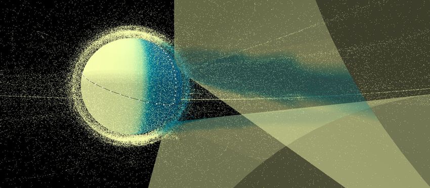
sites is provided in Table 6, while Figure 8 illustrates their global distribution.
Site Country Altitude Sky Magnitude Sunshine Rate Score
Deep Sky West Observatory (NM) USA 2445 m 21.99 74% 8.8 /10
Island Teide Observatory (Canaries) Spain 2357 m 21.41 78% 8.3 /10
Drebach-South Observatory (Tivoli) Namibia 1340 m 22.00 82% 8.1 /10
Deep Sky Chile Chile 1700 m 21.96 66% 7.9 /10
Table 6: Evaluation of the MTOS sites based on 3 criteria: altitude, background sky magnitude and annual sunshine
rate.
Fig. 8: An example of the MTOS network, using the locations presented in Table 6.
To obtain the best global network coverage, it would be crucial to implement MTOS stations in Pacific Polynesia –
one in Hawaii for the Northern hemisphere and one in Tahiti for the Southern hemisphere – to cover at least part of the
Pacific, but also in Eastern Asia and Australia to cover both hemispheres as well.
4.3 Generating synthetic populations
The latest version of the MASTER software developed and maintained by ESA was used to obtain the densities of
resident space objects (RSO) across multiple altitude intervals (or altitude shells) and with minimum sizes varying
Copyright © 2021 Advanced Maui Optical and Space Surveillance Technologies Conference (AMOS) – www.amostech.comAMOS Tech 2021
10 6
10 7
10 8
Density [km 3]
10 9
10 10
10 11
>1 cm >10 cm >30 cm Reconstructed density
10 12 >2 cm >15 cm >40 cm Density extracted from ESA MASTER
>5 cm >20 cm >50 cm
103 104
Altitude [km]
Fig. 9: Space object densities for various sizes as computed by ESA MASTER 2016 software.
from 1 cm to 50 cm. The altitude intervals used in the simulation follow a logarithmic evolution from 200 km to
37 500 km. The software was run for each centimeter between 1 cm and 50 cm. Some of the densities that were
obtained are plotted in Figure 9.
The full distribution of the number of RSO per altitude and size is provided in Appendix. This quantity is called
N(h, d), h being the altitude and d the size. The total number of objects larger than 1 cm is found to be 1 001 826.
For each altitude shell and for each size interval, we need to create a number of objects N(h, d). Since N(h, d) is
deduced from the density and the volume, it is not an integer. A random uniform variable was used to determine
whether bN(h, d)c or bN(h, d)c + 1 should be used, b·c being the mathematical floor function. The position-velocity
(PV) vectors of the synthetic objects were generated using the latest catalog of resident space objects extracted from
space-track.org on January 31st , 2021. For each cataloged object, the PV vectors were obtained using the SGP4
propagator. For each altitude shell, many cataloged RSO were randomly chosen in the corresponding altitude shell.
Their PV vector have then been slightly perturbed and propagated using a Keplerian orbit propagator to be assigned to
one of the synthetic objects. For each synthetic object, a random size d was assigned in the corresponding size interval
(n[cm] < d < n + 1[cm]) using a uniform probability function, for simplicity. The size of objects larger than 50 cm is
described using a cubic uniform (d 1/3 follows a uniform probability function) probability function between 50 cm and
10 m, to account for the greater number of smaller objects.3
This method allows for a reasonable estimate of the RSO populations beyond the cataloged objects without direct
access to the statistical measurements. As a sanity check, the density initially extracted from MASTER (solid lines) is
successfully compared with the density computed from the synthetic populations (dots) in Figure 9.
4.4 Implementation and setup of the MTOS simulator
A full simulator of the sensor network capabilities was developed based on the equations presented in Section 2,
validated in Section 3, incorporating the synthetic populations presented in the previous paragraph propagated over a
period of 28 days. The simulator was developed in Python with an object-oriented approach.
3 Objects larger than 50 cm are usually detected anyway, such that this rough and somewhat arbitrary choice does not affect the general conclu-
sions.
Copyright © 2021 Advanced Maui Optical and Space Surveillance Technologies Conference (AMOS) – www.amostech.comAMOS Tech 2021
Time step 9s
Telescope field of view 4.3◦
Number of time steps 268,800
Physical time of the simulation 28 days
Telescope elevation 40◦
Minimum streak length for detection 50 pixels
Minimum SNR for detection 1.25
Exposure time 300 ms
PSF 1.3 pixels
Table 7: Main common parameters of the simulations.
The orbit propagator is a custom-made vectorized numerical propagator. It is a simple model that incorporates only J2
perturbations on top of the central-force. The acceleration is [15]:
µr 3J2 µR2E
2 2
dv z z
=− 3 + 5 2 − 1 (x ex + y ey ) + z 5 2 − 3 ez (35)
dt r 2r5 r r
where µ is the Earth’s gravitational constant, r = x ex + y ey + z ez is the position vector of the object in geocentric
equatorial coordinates, and J2 = 1.08262668 × 10⁻³ is the coefficient representing the effect of Earth’s oblateness in
the Legendre polynomial representation of Earth’s gravitational field. The need for fast orbit propagation of a large
amount of objects led us to this simplified model that can be implemented very efficiently. The propagation of 83,000
objects over 28 days with a sampling time of 9 s takes 24 hours on a single CPU. The presence of the J2 term is
important because it accounts for the drift of the right ascension of the ascending node (RAAN) which can affect the
visibility of an object from a station over the time of the simulation.
The time step was chosen to be 9 s because it corresponds approximately to the minimum transit time of a LEO object
through the field of view of the camera. Therefore, the rotating telescope system can be modeled as a conic curtain. At
each time step, the visibility of each of the objects from each observation station is assessed based on multiple criteria:
1. The station has to be in the night. The night is defined by the time when the Sun is more than 15◦ below horizon.
2. The object needs to be illuminated by the Sun.
3. The object has to be in the visibility cone of the station, that is, that the angle between the central direction of
the MTOS and the vector between the observatory and the object has to be close to half the global angle of the
station:
θtelescope
|(ustation , AM) − θstation | < (36)
2
4. The SNR, computed with Equation 33, has to be greater than 1.25.
5. The streak has to be at least 50 pixels long.
These criteria are assessed between each object-station pair at each time step. The simulation takes typically 4 days
on 4 CPU, including the orbit propagation. To simplify the simulation setup, all the symmetry axis of each MTOS
point at the local zenith in the simulation. The telescopes are pointing with an elevation of 40◦ . For the simulation, we
use RASA 14” or WMS 1000 telescopes equipped with a GSENSE6060 camera. Simulations were run with a single
station on Tenerife in the Canary islands, and with four stations spread across Northern and Southern hemispheres
across continents: Tenerife, Namibia, New Mexico (USA) and Chile. The influence of the Moon cycle is taken into
account. The simulation is run over the course of 28 days, which corresponds to one full Moon cycle.
Figure 10 illustrates the concept of the simulation at one given time step: the MTOS that are in the night can potentially
detect resident space objects if the received SNR is large enough and the streak obtained is long enough.
Copyright © 2021 Advanced Maui Optical and Space Surveillance Technologies Conference (AMOS) – www.amostech.comAMOS Tech 2021
Minimum SNR = 1.25
-Tenerife : 40° (elevation), 21.5/arcsec², OTA : RASA14
Duration of observation : 672.0 hours (28.0 days)
Total of new RSOs catalogued : 8961 / 15181 observed (59.0%)
Fig. 10: 3D view of the simulation including the detection cones of two MTOS as well as the shaded and illuminated
populations of resident space objects.
4.5 Performance of the MTOS
The simulation of a single RASA 14” telescope station in Tenerife yielded the results shown in Figure 13a and Fig-
ure 14a.
The number of cataloged objects in this configuration reaches 8961 within 28 days of observation. It is important to
know that a RSO is considered cataloged when it has been observed more than 5 times in less than 5 days. Once
an object has been cataloged, a dedicated observation schedule can be built to keep it in the catalog. After 96 hours
(4 days) of detection simulated, we can notice a drop in the increase of detected objects in Figure 14a. This loss of
performance is due to the high brightness of the full Moon which deteriorates that of the night-sky. It has been shown
that its brightness could decrease by up to 3 units of magnitude per squared arc-second, rendering the night sky to a
value of 18.5 mag/arcsec2 . The effect on the RSO cataloging is not as important, the reason being that some objects
are still detected within this time period and that the first or last observations (with better sky conditions4 ) could have
been made before or after the full Moon.
Number of RSO according to their size
6000
Detected RSO (seen at least once)
5000 Catalogued RSO
(seen at least 5 times within 5 days)
Number of RSO
4000
3000
2000
1000
0
3 4 5 6 7 8 9 10 20 30 40 50 60 70 80 90 100 200 300 400 500 600 700 800 9001000
Size range of RSO in cm
Fig. 11: Size range of observed RSO with a single RASA 14 observation station.
Size-wise, it is possible to observe RSO as small as 4 cm. However, optimal observation conditions for objects of this
4 Weather has not been taken into account in the simulation. That means that the sky is clear at all times, and only the Moon has an influence on
the sky conditions. However, given the high annual sunshine rate and altitude of the observation sites in the simulation, neglecting the weather still
gives accurate results and correct estimations of the system performance.
Copyright © 2021 Advanced Maui Optical and Space Surveillance Technologies Conference (AMOS) – www.amostech.comAMOS Tech 2021
Minimum
size SNR =met,
are seldom 1.25 making it highly unlikely for them to meet the cataloging criterion. We can indeed see that for
-Tenerife : 40° (elevation),
objects smaller than 20 cm,21.5/arcsec², OTA :rate
the cataloging RASA14
drops from approximately 80% to 55%, going as low as 10 to 20% for
those under 10 cm in size. In order to be seen, they need to feature a very low phase angle to reflect as much sunlight
Duration of observation : 672.0 hours (28.0 days)
asTotal of new RSOs catalogued : 8961 / 15181 observed (59.0%)
possible.
RSOs by Orbit Category
46255
Objects in reference dataframe (size > 3 cm)
Detected objects (seen at least once)
40000 Catalogued objects (seen at least 5 times within 5 days)
30332
Number of RSOs
30000
20000
10000
6610 7165 7089
14 113 927
646 4021 4294
0
Equatorial HEO Polar SSO Other
SSO objects by Right Ascension of the Asending Node
1200
SSO objects in reference dataframe (size > 3 cm)
Detected SSO objects (seen at least once)
Catalogued objects (seen at least 5 times within 5 days)
1000
Number of RSOs
800
600
400
200
0
0 50 100 150 200 250 300 350
Right Ascension of the Asending Node (°)
Fig. 12: Orbits of observed and cataloged RSO with single observation station. Some objects remain hard to detect,
especially the SSO objects whose RAAN (Right Ascension of the Ascending Node) is between 40◦ and 100◦ . That is
mostly due to the fact that RSO on these orbits are often in Earth’s shadow when passing through the nigh sky.
Figure 12 shows the number of RSO detected and cataloged for each main type of LEO orbit. This gives an idea
of the actual situation in orbit described by ESA MASTER model, but also gives an idea of the performance of the
system, since all the objects in the catalog are shown on the histogram. Moreover, the second graphic shows that SSO
(Sun Synchronous Orbit) detection is limited by the right ascension of the ascending node (RAAN), as part of these
Copyright © 2021 Advanced Maui Optical and Space Surveillance Technologies Conference (AMOS) – www.amostech.comAMOS Tech 2021
orbits can be in Earth’s shadow during almost half of their orbital period. This corresponds to the low number of
detected/cataloged objects whose RAAN varies from 40 to 100◦ . However, these objects still remain detectable as it
can be seen on the histograms, given that they have a low phase angle when observed.
Nevertheless, the detection capabilities of 1 MTOS using a RASA 14 over a 28-day period have not yet been exploited
to their maximum, the reason being that the simulations have not been extended over one full Moon cycle. According
to the trend of the cumulative curves of Figure 13a, the MTOS should be able to detect and catalog many more RSO.
OTA RASA 14” WMS 1000
Number of stations 1 4 1 4
RSO detected 15,181 18,382 48,764 56,597
RSO cataloged 8,961 15,419 40,196 53,010
Cataloging rate 59% 84% 82% 94%
Size min detected [cm] 4 4 3 3
Size min cataloged [cm] 7 5 3 3
Mean latency for next observation [h] 29.4 10.2 24.1 7.7
Table 8: Simulation outputs summary.
4.5.1 Single MTOS vs 4 MTOS network
The detection capabilities of 1 MTOS are quite similar to a 4 MTOS network using the same OTA. We can clearly see
that the benefit of implementing a network lies in the cataloging capabilities of such as system: Using the RASA 14”,
the increase of detected objects is of 21%, whereas the increase of cataloged objects is of 72%. The same applies
for the WMS 1000 stations, however less visible as the detection capabilities of the RASA 14” are far behind the
WMS 1000. Even so, a 4 MTOS network using the latter is able to detect 16% more RSO, while the increase in the
number of cataloged objects is of 32%. This is explained by a lower observation latency for a same RSO as shown in
Table 8, that allows the system to multiply the number of observations and incidentally meet the cataloging criterion.
This low latency can also be viewed on the frequency diagrams of Figure 13, where it is possible to see that the number
of observations for a same RSO tends towards higher values when using a 4 MTOS network.
Another advantage of using a 4 MTOS network is the low effect of the moon on the detection capabilities. By
multiplying the number of station, the conditions of detection – such as a low phase angle, the crossing of the detection
cone – are increased, for the RSO can cross 4 cones on an orbit, raising its chances to be distant from the full moon
and be detected. However, as the WMS 1000’s detection performances outweigh those of the RASA 14”, it is much
less impacted by the moon, regardless of the number of stations. It is possible to contemplate the lessened effect of
the moon due to the higher number of stations on Figure 14.
Copyright © 2021 Advanced Maui Optical and Space Surveillance Technologies Conference (AMOS) – www.amostech.comAMOS Tech 2021
1. Observation Frequency of detected RSOs 1. Observation Frequency of detected RSOs
2. Cumulative Sum of new RSOs seen/catalogued over time 2. Cumulative Sum of new RSOs seen/catalogued over time
1400 Minimum SNR = 1.25 1750 Minimum SNR = 1.25
-Tenerife : 40° (elevation), 21.5/arcsec², OTA : RASA14 -Tenerife : 40° (elevation), 21.5/arcsec², OTA : WMS-1000
1200 Duration of observation : 672.0 hours (28.0 days) 1500 Duration of observation : 672.0 hours (28.0 days)
Total of new RSOs catalogued : 8961 / 15181 observed (59.0%) Total of new RSOs catalogued : 40196 / 48764 observed (82.0%)
1000 1250
n° RSOs Observed
n° RSOs Observed
800 1000
600 750
400 500
200 250
0 0
0 20 40 60 80 100 120 140 0 20 40 60 80 100 120 140
Number of Observations Number of Observations
(a) Observation frequency
1. Observation for single
Frequency MTOS
of detected and RASA 14”
RSOs 50000
(b) Observation frequencyFrequency
1. Observation for Single MTOS
of detected and WMS 1000
RSOs
2. Cumulative Sum of new RSOs seen/catalogued over time 2. Cumulative Sum of new RSOs seen/catalogued over time
14000
n° of new RSO Observed / Catalogued
n° of new RSO Observed / Catalogued
700
12000 40000
Minimum SNR = 1.25 Minimum SNR = 1.25
800
600 -Tenerife : 40° (elevation), 21.5/arcsec², OTA : RASA14 -Tenerife : 40° (elevation), 21.5/arcsec², OTA : WMS-1000
10000 -Namibia : 40° (elevation), 21.5/arcsec², OTA : RASA14 -Namibia : 40° (elevation), 21.5/arcsec², OTA : WMS-1000
-NewMexico : 40° (elevation), 21.5/arcsec², OTA : RASA14 30000 -NewMexico : 40° (elevation), 21.5/arcsec², OTA : WMS-1000
-Chile : 40° (elevation), 21.5/arcsec², OTA : RASA14 -Chile : 40° (elevation), 21.5/arcsec², OTA : WMS-1000
500
8000 600
n° RSOs Observed
n° RSOs Observed
Duration of observation : 672.0 hours (28.0 days) Duration of observation : 672.0 hours (28.0 days)
Total of new RSOs catalogued : 15419 / 18382 observed (84.0%) Total of new RSOs catalogued : 53010 / 56597 observed (94.0%)
6000
400 20000
4000 400
300
10000
2000 New RSOs Detected (observed once) New RSOs Detected (observed once)
200 New RSOs Catalogued New RSOs Catalogued
(observed more than 5 times within less than 5 days) 200 (observed more than 5 times within less than 5 days)
1000 0 100 200 300 400 500 600
0
0 100 200 300 400 500 600
Duration of Observation (hours) Duration of Observation (hours)
0 0
0 50 100 150 200 250 300 350 0 100 200 300 400 500
Number of Observations Number of Observations
(c) Observation frequency for 4 MTOS and RASA 14” (d) Observation frequency for 4 MTOS and WMS 1000
17500
50000 frequency, leading to higher numbers of cataloged
Fig. 13: Influence of the number of stations on the observation
n° of new RSO Observed / Catalogued
n° of new RSO Observed / Catalogued
15000
objects. It is clearly visible that by adding 3 additional MTOS to the network reduces the number of RSO observed
few
12500times and increases the number of RSO observed several 40000
times, by looking at the variations from Figure 13a to
Figure 13c and Figure 13b to Figure 13d.
10000 30000
7500
20000
5000
New RSOs Detected (observed once) 10000 New RSOs Detected (observed once)
2500
New RSOs Catalogued New RSOs Catalogued
(observed more than 5 times within less than 5 days) (observed more than 5 times within less than 5 days)
0 0
0 100 200 300 400 500 600 700 0 100 200 300 400 500 600 700
Duration of Observation (hours) Duration of Observation (hours)
Copyright © 2021 Advanced Maui Optical and Space Surveillance Technologies Conference (AMOS) – www.amostech.comTotal of new RSOs catalogued : 8961 / 15181 observed (59.0%) Total of new RSOs catalogued : 40196 / 48764 observed (82.0%)
1000 1250
n° RSOs Observed
n° RSOs Observed
800 1000
AMOS Tech 2021
600 750
400 500
200 250
0 0
0 20 40 60 80 100 120 140 0 20 40 60 80 100 120 140
Number of Observations Number of Observations
50000
14000
1. Observation Frequency of detected RSOs 1. Observation Frequency of detected RSOs
2. Cumulative Sum of new RSOs seen/catalogued over time 2. Cumulative Sum of new RSOs seen/catalogued over time
n° of new RSO Observed / Catalogued
n° of new RSO Observed / Catalogued
12000 40000
700
10000 Minimum SNR = 1.25 Minimum SNR = 1.25
800
30000
600 -Tenerife : 40° (elevation), 21.5/arcsec², OTA : RASA14 -Tenerife : 40° (elevation), 21.5/arcsec², OTA : WMS-1000
8000 -Namibia : 40° (elevation), 21.5/arcsec², OTA : RASA14 -Namibia : 40° (elevation), 21.5/arcsec², OTA : WMS-1000
-NewMexico : 40° (elevation), 21.5/arcsec², OTA : RASA14 -NewMexico : 40° (elevation), 21.5/arcsec², OTA : WMS-1000
-Chile : 40° (elevation), 21.5/arcsec², OTA : RASA14 -Chile : 40° (elevation), 21.5/arcsec², OTA : WMS-1000
500
6000 20000
600
n° RSOs Observed
n° RSOs Observed
Duration of observation : 672.0 hours (28.0 days) Duration of observation : 672.0 hours (28.0 days)
Total of new RSOs catalogued : 15419 / 18382 observed (84.0%) Total of new RSOs catalogued : 53010 / 56597 observed (94.0%)
400
4000
10000
New RSOs Detected (observed once) 400 New RSOs Detected (observed once)
300
2000
New RSOs Catalogued New RSOs Catalogued
(observed more than 5 times within less than 5 days) (observed more than 5 times within less than 5 days)
2000 0 100 200 300 400 500 600
0
0 100 200 300 400 500 600
200
100 Duration of Observation (hours) Duration of Observation (hours)
(a) Cumulative
0 RSO detected/observed for single MTOS with (b) Cumulative
0 RSO detected/observed for single MTOS with
RASA 14”0 50 100 150 200 250 300 350 WMS 10000 100 200 300 400 500
Number of Observations Number of Observations
17500
50000
n° of new RSO Observed / Catalogued
n° of new RSO Observed / Catalogued
15000
12500 40000
10000 30000
7500
20000
5000
New RSOs Detected (observed once) 10000 New RSOs Detected (observed once)
2500
New RSOs Catalogued New RSOs Catalogued
(observed more than 5 times within less than 5 days) (observed more than 5 times within less than 5 days)
0 0
0 100 200 300 400 500 600 700 0 100 200 300 400 500 600 700
Duration of Observation (hours) Duration of Observation (hours)
(c) Cumulative RSO detected/observed for 4 MTOS with (d) Cumulative RSO detected/observed for 4 MTOS with
RASA 14” WMS 1000
Fig. 14: Comparison of the influence of the full Moon on RSO detection. On Figure 14a, the effect of the moon on
the number of RSO observed is visible when using a single MTOS and RASA 14”, whereas the addition of 3 stations
decreases its influence as seen on Figure 14c, for the same OTA. When comparing the effect of the Moon using a more
efficient OTA such as the WMS 1000, the effect of the moon is much less visible, but still remains emphasized when
considering a single MTOS as in Figure 14b rather than a 4 MTOS network as in Figure 14d.
Copyright © 2021 Advanced Maui Optical and Space Surveillance Technologies Conference (AMOS) – www.amostech.comYou can also read