Quantifying memory and persistence in the atmosphere-land and ocean carbon system
←
→
Page content transcription
If your browser does not render page correctly, please read the page content below
Research article
Earth Syst. Dynam., 13, 439–455, 2022
https://doi.org/10.5194/esd-13-439-2022
© Author(s) 2022. This work is distributed under
the Creative Commons Attribution 4.0 License.

                   Quantifying memory and persistence in the
                   atmosphere–land and ocean carbon system
                        Matthias Jonas1 , Rostyslav Bun2,3 , Iryna Ryzha2 , and Piotr Żebrowski1
               1 Advancing Systems Analysis Program, International Institute for Applied Systems Analysis,
                                               2361, Laxenburg, Austria
             2 Department of Applied Mathematics, Lviv Polytechnic National University, 79013, Lviv, Ukraine
          3 Department of Transport and Computer Sciences, WSB University, 41300, Dabrowa
                                                                                        ˛     Górnicza, Poland
                                   Correspondence: Matthias Jonas (jonas@iiasa.ac.at)

                                     Received: 22 April 2021 – Discussion started: 1 July 2021
                        Revised: 31 January 2022 – Accepted: 4 February 2022 – Published: 10 March 2022

      Abstract. Here we intend to further the understanding of the planetary burden (and its dynamics) caused by
      the effect of the continued increase in carbon dioxide (CO2 ) emissions from fossil fuel burning and land use as
      well as by global warming from a new rheological (stress–strain) perspective. That is, we perceive the emission
      of anthropogenic CO2 into the atmosphere as a stressor and survey the condition of Earth in stress–strain units
      (stress in units of Pa, strain in units of 1) – allowing access to and insight into previously unknown characteristics
      reflecting Earth’s rheological status. We use the idea of a Maxwell body consisting of elastic and damping
      (viscous) elements to reflect the overall behavior of the atmosphere–land and ocean system in response to the
      continued increase in CO2 emissions between 1850 and 2015. Thus, from the standpoint of a global observer, we
      see that the CO2 concentration in the atmosphere is increasing (rather quickly). Concomitantly, the atmosphere
      is warming and expanding, while some of the carbon is being locked away (rather slowly) in land and oceans,
      likewise under the influence of global warming.
         It is not known how reversible and how out of sync the latter process (uptake of carbon by sinks) is in relation
      to the former (expansion of the atmosphere). All we know is that the slower process remembers the influence
      of the faster one, which runs ahead. Important questions arise as to whether this global-scale memory – Earth’s
      memory – can be identified and quantified, how it behaves dynamically, and, last but not least, how it interlinks
      with persistence by which we understand Earth’s path dependency.
         We go beyond textbook knowledge by introducing three parameters that characterize the system: delay time,
      memory, and persistence. The three parameters depend, ceteris paribus, solely on the system’s characteristic
      viscoelastic behavior and allow deeper and novel insights into that system. The parameters come with their own
      limits which govern the behavior of the atmosphere–land and ocean carbon system, independently from any
      external target values (such as temperature targets justified by means of global change research). We find that
      since 1850, the atmosphere–land and ocean system has been trapped progressively in terms of persistence (i.e.,
      it will become progressively more difficult to relax the system), while its ability to build up memory has been
      reduced. The ability of a system to build up memory effectively can be understood as its ability to respond still
      within its natural regime or, if the build-up of memory is limited, as a measure for system failures globally in the
      future. Approximately 60 % of Earth’s memory had already been exploited by humankind prior to 1959. Based on
      these stress–strain insights we expect that the atmosphere–land and ocean carbon system will be forced outside
      its natural regime well before 2050 if the current trend in emissions is not reversed immediately and sustainably.

Published by Copernicus Publications on behalf of the European Geosciences Union.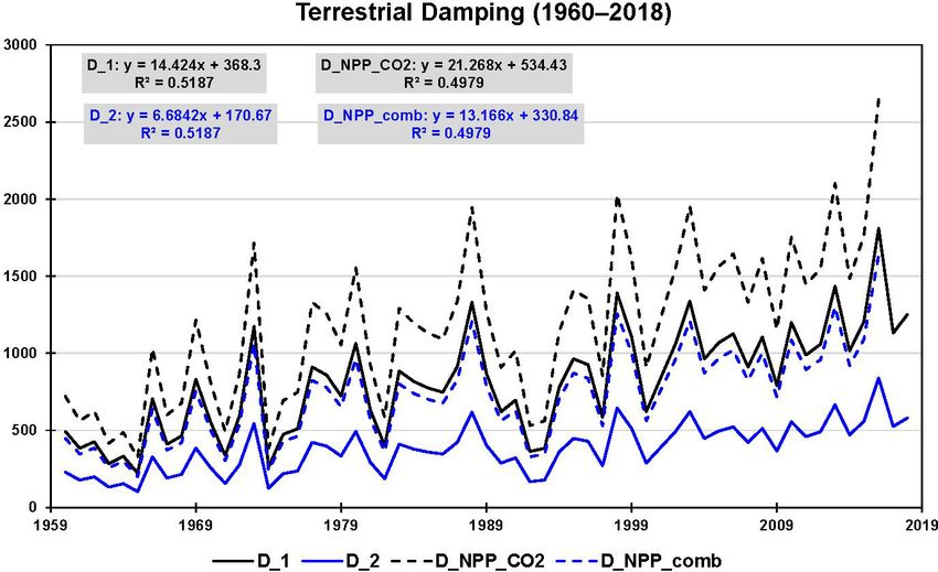
440               M. Jonas et al.: Quantifying memory and persistence in the atmosphere–land and ocean carbon system

1   Motivation                                                       sinks, as the overall strain response of the atmosphere–land
                                                                     and ocean carbon system.
                                                                        It is not known how reversible and how out of sync the
Over the last century anthropogenic pressure on Earth be-            latter process (uptake of carbon by sinks) is in relation to the
came increasingly noticeable. Human activities turned out            former (expansion of the atmosphere) (Boucher et al., 2012;
to be so pervasive and profound that the very life support           Dusza et al., 2020; Garbe et al., 2020; Schwinger and Tjipu-
system upon which humans depend is threatened (Steffen et            tra, 2018; Smith, 2012). All we know is that the slower pro-
al., 2004, 2015). The increase in emissions of greenhouse            cess remembers the influence of the faster one, which runs
gases (GHGs) into the atmosphere is only one of several se-          ahead. Three (nontrivial) questions arise: (1) can this global-
rious global threats, and their reduction is at the center of        scale memory – Earth’s memory – be quantified? (2) Can
international agreements (Steffen et al., 2015; UN Climate           Earth’s memory be compared with a buffer which is limited
Change, 2022; UN Sustainable Development Goals, 2022).               and negligently exploited; that is, what is the degree of de-
   Here we intend to further the understanding of the plan-          pletion? And (3) does Earth’s memory allow its persistence
etary burden (and its dynamics) caused by the effect of the          (path dependency) to be quantified, speculating that the two
continued increase in GHG emissions and by global warm-              are not independent of each other? We answer these ques-
ing from a new rheological (stress–strain) perspective. That         tions in the course of our paper.
is, we perceive the emission of anthropogenic GHGs, no-                 This suggests, as the next step in developing a stress–strain
tably carbon (CO2 ), into the atmosphere as a stressor. This         systems perspective, getting a grip on Earth’s memory. To
perspective goes beyond the global carbon mass balance per-          this end, we focus on the slow-to-fast temporal offset inher-
spective applied by the carbon community, which is widely            ent in the atmosphere–land and ocean system, while prefer-
referred to as the gold standard in assessing whether Earth          ring an approach which is reduced to the highest possible ex-
will remain hospitable for life (Global Carbon Project, 2019).       tent; however, we do so without compromising complexity
There, the condition of Earth is surveyed in units of peta-          in principle. To this end, it is sufficient to resolve subsys-
grams of carbon per year (Pg C yr−1 ), while we survey its           tems as a whole and to perceive their physical reaction in re-
condition in stress–strain units (stress in units of Pa, strain in   sponse to the increase in atmospheric CO2 concentrations as
units of 1) – allowing access to and insight into previously         a combined one (i.e., including effects such as that of global
unknown characteristics reflecting Earth’s rheological status.       warming). From a temporal perspective, the subsystems’ re-
   We note that – although the focus is on the atmosphere–           actions, the expansion of the atmosphere by volume and the
land and ocean carbon system – the stress–strain approach            sequestration of carbon by sinks, can be considered suffi-
described herein should not be considered an appendix to a           ciently disjunct. Under optimal conditions (referring to the
mass-balance-based carbon cycle model. Instead, it leads to          long-term stability of the temporal offset), the temporal offset
a self-standing model belonging to the suite of reduced but          view even suggests that we can refrain from disentangling the
still insightful models (such as radiation transfer, energy bal-     exchange of both thermal energy and carbon throughout the
ance, or box-type carbon cycle models), which offer great            atmosphere–land and ocean system, as is done in climate–
benefits in safeguarding complex three-dimensional climate           carbon models ranging from reduced to complex (Flato et al.,
and global change models. A stress–strain model is missing           2013; Harman and Trudinger, 2014). The additional degree
in that suite of support models. Here we demonstrate the ap-         of reductionism, whilst preserving complexity, will prove an
plicability and efficacy of such a model in an Earth systems         advantage in advancing our understanding of the temporal
context.                                                             offset in terms of memory and persistence.
   To develop a stress–strain systems perspective, we begin             In view of the aforementioned questions, we chose a rheo-
with the stress given by the CO2 emissions from fossil fuel          logical stress–strain (σ –ε) model (Roylance, 2001; TU Delft,
burning and land use between 1959 and 2015 (with the in-             2022): a Maxwell body (MB) consisting of an elastic element
crease between 1850 and 1958 serving as antecedent or up-            (its constant, traditionally denoted E for Young’s modulus,
stream emissions). Thus, from the standpoint of a global             is replaced by the compression modulus K) and a damping
observer, we see that the CO2 concentration in the atmo-             (viscous) element (the damping constant is denoted D) to
sphere is increasing (rather quickly). Concomitantly, the at-        capture the stress–strain behavior of the global atmosphere–
mosphere is warming (here combining the effect of tropo-             land and ocean system (Fig. 1) and to simulate how hu-
spheric warming and stratospheric cooling) and expanding             mankind propelled that global-scale experiment historically.
(by approximately 15–20 m in the troposphere per decade              We note that the MB is a logical choice of model given the
since 1990), while some of the carbon is being locked away           uninterrupted increase in atmospheric CO2 concentrations
(rather slowly) in land and oceans, likewise under the in-           since 1850 (Global Carbon Project, 2019).
fluence of global warming (Global Carbon Project, 2019;                 In practice, rheology is principally concerned with extend-
Lackner et al., 2011; Philipona et al., 2018; Steiner et al.,        ing continuum mechanics to characterize the flow of materi-
2011, 2020). We refer to these two processes together, the           als that exhibit a combination of elastic, viscous, and plastic
expansion of the atmosphere and the uptake of carbon by              behavior (that is, including hereditary behavior) by properly

Earth Syst. Dynam., 13, 439–455, 2022                                                   https://doi.org/10.5194/esd-13-439-2022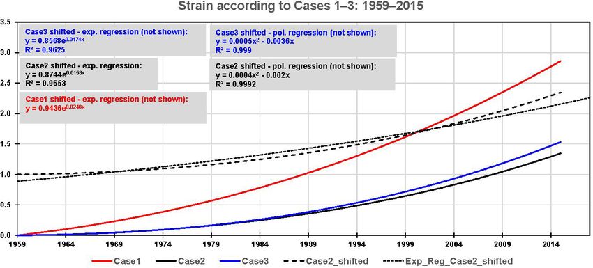
M. Jonas et al.: Quantifying memory and persistence in the atmosphere–land and ocean carbon system                                  441

                                                                      (quasi-continuously), the strain can be expected to be expo-
                                                                      nential or close to exponential. In addition, we provide in-
                                                                      dependent estimates of the likewise unknown compression
                                                                      and damping characteristics of the MB. This a priori knowl-
                                                                      edge allows Eqs. (1a) and (1b) to be used stepwise in combi-
                                                                      nation to narrow down our initial estimate of the K/D ra-
                                                                      tio in particular. More accurate knowledge of this ratio is
                                                                      needed when we go beyond textbook knowledge by distill-
                                                                      ing three parameters – delay time (reflecting the temporal
                                                                      offset mentioned above), memory, and persistence – from
                                                                      the stress-explicit equation. The three parameters depend, ce-
                                                                      teris paribus, solely on the system’s characteristic K/D ra-
                                                                      tio and allow deeper and novel insights into that system. We
Figure 1. Rheological model to capture the stress–strain behav-       see the atmosphere–land and ocean system as being trapped
ior of the global atmosphere–land and ocean system as a Maxwell       progressively over time in terms of persistence. Given its re-
body consisting of elastic (atmosphere) and damping (land–ocean)      duced ability to build up memory, we expect system failures
elements. The stress (in units of Pa; known) is given by the car-     globally well before 2050 if the current trend in emissions
bon (CO2 ) emissions from fossil fuel burning and land use, while     is not reversed immediately and sustainably. Put differently,
the strain (in units of 1; assumed exponential, otherwise unknown)    the stress–strain approach comes with its own internal lim-
is given by the expansion of the atmosphere by volume and uptake      its which govern the behavior of the atmosphere–land and
of CO2 by sinks. Independent estimates of K and D, the compres-       ocean carbon system independently from any external tar-
sion and damping characteristics of the MB, allow its stress–strain   get values (such as temperature targets justified by means of
behavior to be captured and adjusted until consistency is achieved
                                                                      global change research).
(see text).
                                                                         There is a wide range of other approaches which aim at
                                                                      exploring memory and persistence in Earth systems data,
combining elasticity and (Newtonian) fluid mechanics. Lim-            typically with the focus on individual Earth subsystems or
its (e.g., viscosity limits) exist beyond which basic rheolog-        processes (e.g., atmospheric temperature or carbon dioxide
ical models are recommended to be refined. However, these             emissions). So far, applied approaches have mainly been
limits are fluent, and basic rheological models also produce          based on classical time series and time–space analyses to
useful results beyond these limits (Malkin and Isayev, 2017;          uncover the memory or causal patterns contained in obser-
Mezger, 2006; TU Delft, 2022).                                        vational data (Barros et al., 2016; Belbute and Pereira, 2017;
   The mathematical treatment of an MB is standard. De-               Caballero et al., 2002; Franzke, 2010; Lüdecke et al., 2013).
pending on whether the strain (ε) or the stress (σ ) is known         However, these approaches come with well-known limita-
(in addition to the compression and damping characteris-              tions which can all be attributed, directly or indirectly, to the
tics K and D), the stress–strain equation describing the              issue of forecasting (more precisely, the conditions placed
MB between 0 and t can be applied in a stress-explicit form,          on the data to enable forecasting) or are not based on physics
                                                                      (Aghabozorgi et al., 2015; Darlington, 1996; Darlington and
                       Zt                                         Hayes, 2016). By way of contrast, we do not forecast. We
                   K                   K
σ (t) = σ (0) exp − t + K ε̇(τ ) exp     (τ − t) dτ ,         (1a)    perpetuate long-term historical conditions which, in turn, al-
                   D                   D
                                0                                     lows the delay time in the atmosphere–land and ocean sys-
                                                                      tem to be expressed analytically in terms of memory and
or in a strain-explicit form,
                                                                      persistence. We are not aware of any scientific discipline or
                                       Zt                             research area in which memory and persistence are defined
             1                  1                                     other than statistically and are interlinked, if at all, other than
ε(t) = ε(0) + [σ (t) − σ (0)] +             σ (τ )dτ,         (1b)
             K                  D                                     via correlation.
                                       0
                                                                         Rheological approaches are common in Earth systems
with σ (0) and ε(0) denoting initial conditions and a dot             modeling as well. Typically, they are applied to mimic the
the derivative by time (Roylance, 2001; Bertram and Glüge,            long(er)-term behavior of Earth subsystems, e.g., its mantle
2015).                                                                viscosity, which is crucial for interpreting glacial uplift re-
   Here, we focus on the application of these equations in            sulting from changes in planetary ice sheet loads (Müller,
an atmosphere–land and ocean carbon context. For an ob-               1986; Whitehouse et al., 2019; Yuen et al., 1986). Yet, to the
server it is the overall strain response of that system (ex-          best of our knowledge, a rheological approach to unravel the
pansion of the atmosphere by volume and uptake of CO2                 memory and persistence behavior of the global atmosphere–
by sinks) that is unknown. However, since atmospheric CO2             land and ocean system in response to the long-lasting in-
concentrations have been observed to increase exponentially

https://doi.org/10.5194/esd-13-439-2022                                                   Earth Syst. Dynam., 13, 439–455, 2022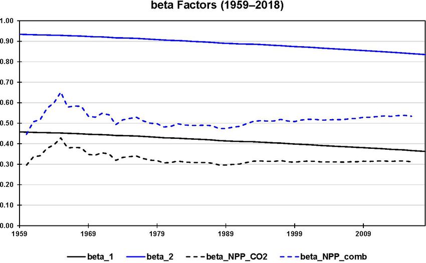
442                M. Jonas et al.: Quantifying memory and persistence in the atmosphere–land and ocean carbon system

crease in atmospheric CO2 emissions had not been applied           to ensure that exponents still come in units of 1 after we split
                                                                                                                           t
before.                                                            them up, we introduce the dimensionless time n = 1t       glob-
   We describe our rheological model (MB) approach in de-          ally (which will be discretized in the sequel when we refer to
tail in Sect. 2, while we provide an overview of the applied       a temporal resolution of 1 year and set 1t = 1 yr) such that,
                                                                                                    n
data and conversion factors in Sect. 3. In Sect. 4 we describe     for example, q t = exp − K D 1t .
how we derive first-order estimates of the main characteris-          To understand the systemic nature of the MB, we explore
tics of the atmosphere–land and ocean system (in terms of          its stress dependence on q = exp − K    D 1t , which contains
the MB’s K and D characteristics) by using available knowl-        the ratio of K and D, the two characteristic parameters of the
edge. Although uncertain, these estimates become useful in         MB, by way of derivation by q (while α is held constant). To
Sect. 5 where we apply the aforementioned stress- and strain-      this end, we transform Eq. (2a) further to
explicit equations to quantify delay time, memory, and per-
                                                                                  1        1
sistence of the atmosphere–land and ocean system. We con-          σD (q, t) :=     σ (t) = σ (n) =: σD (q, n)                 (2b)
clude by taking account of our main findings in Sect. 6.                          D        D
                                                                                ∂
                                                                   and execute ∂q σD (q, n), the derivation by q of the system’s
2   Method                                                         rate of change σD (which is given in units of yr−1 ). Doing
                                                                   so allows (what we call) delay time T to be distilled (see
This section provides an overview of how we process                Supplement Information 2). It is defined as
Eq. (1a) and how we distill delay time, memory, and per-
sistence from this equation. To familiarize oneself with the                      qβ ∂Sn      qβn        qβ
                                                                   T (q, n) :=           =−         n+        ,                 (3)
details, the reader is referred to the Supplement.                                Sn ∂qβ    1 − qβn    1 − qβ
   To start with, we assume that we know the order of magni-
tude of both the K/D ratio characteristic of the atmosphere–       where qβ = qα q, qα = exp(−α1t), and Sn = S(q, n) =
                                                                   1−qβn
land and ocean system and the rate of change in the strain ε       1−qβ .   The delay time behaves asymptotically for increas-
given by ε̇(t) = α exp(αt) with the exponential growth factor      ing n and approaches T∞ = lim T =
                                                                                                             qβ
α > 0. These first-order estimates permit Eqs. (1a) and (1b)                                      n→∞       1−qβ .   We further de-
to be used stepwise in combination.                                fine
   Equation (1a): we vary both K/D and α to reproduce              M := S(q, n),                                                (4)
the known stress σ given by the CO2 emissions from fossil
                                                                                     1
fuel burning (fairly well known) and land use (less known)         with M∞ =       1−qβ ,   and
(Global Carbon Project, 2019).
   Equation (1b): we insert both the fine-tuned K/D ratio          P := T (q, n)−1 ,                                            (5)
and the known stress σ to compute the strain ε and check its                                1−q
derivative by time.                                                with P∞ = T1∞ = qβ β as the MB’s characteristic memory
   We consider this procedure a check of consistency, not a        and persistence, respectively. As is commonly done, we keep
proof of concept.                                                  the list of independent parameters minimal. (We only al-
   Delay time, memory, and persistence are characteristic          low K and D – i.e., q – in addition to n; see Eqs. 2b and 3–5
(functions) of the MB. They are contained in the integral on       in particular.)
the right side of Eq. (1a) and are defined independently of ini-      T as given by Eq. (3) is not simply characteristic of the
tial conditions. These appear only in the lower boundary of        MB described by Eqs. (2a) and (2b); it can be shown to ap-
that integral, which allows initial conditions other than zero     pear as delay time in the argument of any function dependent
to be considered by taking advantage of the integral’s addi-       on current and previous times, with a weighting decreasing
tivity. Thus, without loss of generality, we rewrite Eq. (1a)      exponentially backward in time (see Supplement Informa-
for σ (0) = 0, which results in                                    tion 3). Equation (4) reflects the history the MB was ex-
                                                                   posed to systemically prior to current time n (during which
          D
                                                                   α was constant; see Supplement Information 4). Put simply,
σ (t) =     ε̇(t) 1 − qβt ,                                (2a)
          β                                                        M can be understood as the depreciated (q-weighted) strain
                                                                   summed up backward in time. Equation (5) can be shortened
                                                D
(see Supplement Information 1) where β = 1+ K     α and qβt =      to T ·P = 1. If we assume that q can be changed in retrospect
        K                 D

exp − D βt . The term Kβ represents a time characteristic          at n = 0, this equation tells us that if T – that is, 1M per 1q
of the MB under (here) exponential strain (i.e., of the MB         (or, likewise, 1M/M per 1q/q; see the first part of Eq. 3) –
                                                     D
that responds to the stress acting upon it), whereas K  is the     is small, P is great because the change in the system’s char-
relaxation time of the MB (i.e., of the MB that relaxes un-        acteristics (contained in q) hardly influences the MB’s past,
hindered after the stress causing that strain has vanished or      with the consequence that the past exhibits a great path de-
that responds to strain held constant over time; also known        pendency, and vice versa. We therefore perceive persistence
as the relaxation test; Bertram and Glüge, 2015). However,         and path dependency as synonymous.

Earth Syst. Dynam., 13, 439–455, 2022                                                   https://doi.org/10.5194/esd-13-439-2022
M. Jonas et al.: Quantifying memory and persistence in the atmosphere–land and ocean carbon system 443
An additional quantity to monitor is ln(M · P ), which ap- Compared to the reaction of the atmosphere to global warm-
proaches λβ = λ · β for increasing n, with λ = K D 1t as the ing (an expansion of the atmosphere by volume), we consider
characteristic rate of change in the MB. The ratio λ/ ln(M ·P ) this process to be long(er) term in nature and perceive it as a
allows monitoring of how much the system’s natural rate of Newton-like (damping) element.
change is exceeded as a consequence of the continued in- Biospheric carbon uptake is described by the biotic growth
crease in stress (see Supplement Information 5). factor:
1NPP/NPP
3 Data and conversion factors βb = , (6)
1CO2 /CO2
A detailed overview of the carbon data and conversion fac- which is used to approximate the fractional increase in net
tors used in this paper (and also by the carbon community) primary productivity (NPP) per unit increase in atmospheric
is given in Supplement Information 6. The data pertain to CO2 concentration (Wullschleger et al., 1995; Amthor and
atmosphere, land, and oceans: Koch, 1996; Luo and Mooney, 1996). Here we make use of
the model-derived NPP time series (1900–2016) provided by
– atmospheric CO2 concentration (in ppm);
O’Sullivan et al. (2019) to calculate βb (O’Sullivan et al.,
– CO2 emissions from fossil fuel combustion and cement 2019). To understand the uncertainty range underlying βb
production (in Pg C yr−1 ); for 1959–2018, we use the photosynthetic beta factor:
– land use change emissions (in Pg C yr−1 ); dPh CO2
βPh = CO2 L = , (7)
Ph dCO2
– net primary production (in Pg C yr−1 ); and
where L is the so-called leaf-level factor denoting the rela-
– dissolved organic carbon (in µmol kg−1 ).
tive leaf photosynthetic response to a 1 ppmv change in the
They are given by source and time range and are also de- atmospheric concentration of CO2 , bounded by
scribed briefly. The context within which they are used is
revealed in each of the following sections. The conversion L1 ≤ L = f (CO2 ) ≤ L2 , (8)
factors are standard; they are needed to convert C to CO2
(see below), and Ph is the global photosynthetic carbon influx
and parts per million by volume (ppmv) CO2 to petagrams
(i.e., gross primary productivity). Equation (7) is similar to
of carbon (Pg C) or pascal (Pa).
Eq. (6). In Eq. (6) βb represents biomass production changes
in response to CO2 changes, whereas in Eq. (7) βPh describes
4 Independent estimates of D and K photosynthesis changes in response to CO2 changes (Luo and
Mooney, 1996).
In this section we provide independent estimates of the L can be shown to be independent of plant characteristics,
damping and compression characteristics of the atmosphere– light, and the nutrient environment and to vary little by ge-
land and ocean system, with DL and DO denoting the damp- ographic location or canopy position. Thus, L is virtually a
ing constants assigned to land and oceans, respectively, and constant across ecosystems and a function of time-associated
K denoting the compression modulus assigned to the atmo- changes in atmospheric CO2 only (Luo and Mooney, 1996).
sphere. We capture the characteristics’ right order of magni- We use Eq. (7) to test whether βb falls within the
tude only – which can be done on physical grounds by eval- range of βPh given by the quantifiable photosynthetic lim-
uating the combined (net) strain response of each subsystem its L1 (photosynthesis limited by electron transport) and
on the grounds of increasing CO2 concentrations in the atmo- L2 (photosynthesis limited by RuBisCO activity). Figure 2
sphere. These first-order estimates are adequate as they allow shows the biotic growth factors from O’Sullivan et al. (2019)
sufficient flexibility for Sect. 5, where we narrow down our that consider changes in NPP due to the combined effect of
initial estimates by using Eqs. (1a) and (1b) stepwise in com- CO2 fertilization, nitrogen deposition, climate change, and
bination to achieve consistency. carbon–nitrogen synergy (βNPP_comb ) as well as due to CO2
fertilization (βNPP_CO2 ) only. For 1960–2016, βNPP_comb falls
4.1 Estimating the damping constant DL between β1 := βPh (L1 ) and β2 := βPh (L2 ), closer to β1 than
to β2 , whereas βNPP_CO2 even falls below the lower β1 limit.
Increasing concentrations of CO2 in the atmosphere trigger
Rewriting Eq. (7) in the form
the uptake of carbon by the terrestrial biosphere. The intri-
cacies of this process, including potential (positive and nega- 1Phi
tive) feedback processes, are widely discussed (Dusza et al., = Li 1CO2 (i = 1, 2) (9)
Ph
2020; Heimann and Reichstein, 2008; Smith, 2012). The cru-
cial question is how we have observed the process of carbon with Ph = 120 Pg C yr−1 indicates that the additional amount
uptake by the terrestrial biosphere taking place in the past. of annual relative photosynthetic carbon influx, stimulated by
https://doi.org/10.5194/esd-13-439-2022 Earth Syst. Dynam., 13, 439–455, 2022444 M. Jonas et al.: Quantifying memory and persistence in the atmosphere–land and ocean carbon system
Figure 2. Using the lower (β1 ) and upper (β2 ) limits of the photosynthetic beta factor to test the range of the biotic growth factor (βb )
for 1960–2016. The biotic growth factor is derived with the help of modeled net primary production (NPP) values accounting for CO2
fertilization, nitrogen deposition, climate change, and carbon–nitrogen synergy. βNPP_CO2 refers to O’Sullivan et al. (2019), who consider
the change in NPP due to CO2 fertilization only, and βNPP_comb refers to the change in NPP due to the combined effect. All beta factors are
in units of 1.
a yearly increase in atmospheric CO2 concentration, can be Repeating the same procedure for 1959–2016 with
estimated by Li or the sequence of Li if 1CO2 spans mul- O’Sullivan et al. (2019) model-derived NPP values consid-
tiple years (see Supplement Information 7 and Supplement ering the change in NPP due to CO2 fertilization as well as
Data 1). Plotting 1Phi /Ph against time allows lower and up- the total change in NPP, we find
per slopes (rates of strain)
d 1NPP
≈ 0.0013 yr−1 (12a)
d 1Ph1 dt NPP CO2
≈ 0.0019 yr−1 (10a)
dt Ph and
and d 1NPP
≈ 0.0021 yr−1 (12b)
d 1Ph2
dt NPP comb
≈ 0.0041 yr−1 (10b)
dt Ph (linear fits still work well), and consequently
to be derived for 1959–2018. A linear fit works well in either DCO2 ≈ (1172 ± 617) ppmv yr = (119 ± 62) Pa yr
case. The cumulative increase in atmospheric CO2 concen- = (3746 ± 1971)106 Pa s, (13a)
tration since 1959, 1CO2 = CO2 (t) − CO2 (1959), exhibits a
moderate exponential (close to linear) trend. Thus, plotting Dcomb ≈ (726 ± 382) ppmv yr = (74 ± 39) Pa yr
annual changes in CO2 , normalized on the aforementioned = (2319 ± 1220)106 Pa s. (13b)
rates of strain, versus time allows the remaining (moderate)
trends to be interpreted alternatively, namely as average pho- As before, these estimates are closer to the lower leaf-level
tosynthetic damping constants with appropriate uncertainty factor (higher photosynthetic D) than to the higher leaf-level
given by half the maximal range (see Fig. 3 and Supplement factor (lower photosynthetic D; Fig. 3).
Data 1). Here we interpret the O’Sullivan et al. (2019) Earth sys-
tems model as a typical one, which means that the NPP
D1 ≈ (815 ± 433) ppmv yr = (83 ± 44) Pa yr changes it produces are common. We therefore (and suffi-
cient for our purposes) choose the damping constant D1 as
= (2606 ± 1383)106 Pa s (11a)
a good estimator in light of the total change in NPP of the
D2 ≈ (378 ± 201) ppmv yr = (38 ± 20) Pa yr terrestrial biosphere since 1960. Hence,
= (1207 ± 641)106 Pa s. (11b) DL ≈ (815 ± 433) ppmv yr = (83 ± 44) Pa yr
= (2606 ± 1383)106 Pa s. (14)
Earth Syst. Dynam., 13, 439–455, 2022 https://doi.org/10.5194/esd-13-439-2022M. Jonas et al.: Quantifying memory and persistence in the atmosphere–land and ocean carbon system 445
Figure 3. Terrestrial carbon uptake perceived as damping (in ppmv yr) based on the limits of leaf photosynthesis (1960–2018: D1 and D2 )
and on model-derived changes in net primary production (NPP; 1960–2016) due to the combined effect of CO2 fertilization, nitrogen
deposition, climate change, and carbon–nitrogen synergy (DNPP_comb ) as well as CO2 fertilization only (DNPP_CO2 ). The linear trends of
the four damping series are shown at the top. These are used to interpret damping as constants with appropriate uncertainty (given by half
the maximal range).
DL is on the order of viscosity indicated for bitumen and
asphalt (Mezger, 2006). 1DIC
≈ [0.8; 1.9] µmol kg−1 yr−1 , (16)
1t
4.2 Estimating the damping constant DO 1R
≈ [0.01; 0.03] yr−1 (17)
1t
Increasing concentrations of CO2 in the atmosphere trigger
the uptake of carbon by the oceans (National Oceanic and (see also Supplement Data 2). Here it is sufficient to pro-
Atmospheric Administration, 2015). Like the uptake of car- ceed with spatiotemporal averages. As before, the cumula-
bon by the terrestrial biosphere, we consider this process to tive increase in atmospheric CO2 concentration since 1983,
behave like a Newton (damping) element in our MB because 1pCO2 = pCO2 (t) − pCO2 (1983), exhibits a moderate ex-
of the de facto irreversibility on the shorter timescale we are ponential (close to linear) trend. Thus, plotting annual
interested in (Schwinger and Tjiputra, 2018). changes in pCO2 , normalized on the rates of strain
(1DIC/DIC)
The Revelle (buffer) factor (R) quantifies how much at- 1t , versus time allows the remaining (moderate)
mospheric CO2 can be absorbed by homogeneous reaction trend to be interpreted alternatively, namely as an aver-
with seawater. R is defined as the fractional change in CO2 age oceanic damping constant with appropriate uncertainty
relative to the fractional change in dissolved inorganic car- given by half the maximal range (see Fig. 4 and Supplement
bon (DIC): Data 2):
1pCO2 /pCO2 DO ≈ (3005 ± 588) ppmv yr = (304 ± 60) Pa yr
R= . (15)
1DIC/DIC = (9602 ± 1877)106 Pa s. (18)
(Here, in contrast to before, atmospheric CO2 is referred to in DO is on the order of viscosity indicated for bitumen and
units of µatm and therefore indicated by pCO2 .) An R value asphalt, yet approximately 3.7 times greater than DL .
of 10 indicates that a 10 % change in atmospheric CO2 is
required to produce a 1 % change in the total CO2 content of
4.3 Estimating the compression modulus K
seawater (Bates et al., 2014; Egleston et al., 2010; Emerson
and Hedges, 2008). The long-lasting increase in GHG emissions has caused
DIC and R have been observed at seven ocean carbon time the CO2 concentration in the atmosphere to increase and
series sites for periods from 15 to 30 years (between 1983 the atmosphere as a whole to warm (with tropospheric
and 2012) to change slowly and linearly with time (Bates et warming outstripping stratospheric cooling) and to expand
al., 2014): (in the troposphere by approximately 15–20 m per decade
https://doi.org/10.5194/esd-13-439-2022 Earth Syst. Dynam., 13, 439–455, 2022446 M. Jonas et al.: Quantifying memory and persistence in the atmosphere–land and ocean carbon system
Figure 4. Oceanic carbon uptake perceived as damping (in ppmv yr) based on observations at seven ocean carbon time series sites for periods
from 15 to 30 years (between 1983 and 2012). The linear trend in oceanic damping, shown at the bottom, is used to interpret damping as a
constant with appropriate uncertainty (given by half the maximal range).
since 1990) (Global Carbon Project, 2019; Lackner et al.,
2011; Philipona et al., 2018; Steiner et al., 2011, 2020). Our 1
κad = (20b)
whole-subsystem (net-warming) view does not invalidate the γp
known facts that CO2 in the atmosphere is well-mixed (ex-
cept for very low altitudes at which deviations from uniform in the dry adiabatic case, in which γ is the isentropic coeffi-
CO2 concentrations are caused by the dynamics of carbon cient of expansion. Its value is 1.403 for dry air (1.310 for
sources and sinks) and that the volume percentage of CO2 CO2 ) under standard temperature (273.15 K) and pressure
in the atmosphere stays almost constant up to high altitudes (1 atm; 101.325 kPa) (Wark, 1983). We consider a carbon-
(Abshire et al., 2010; Emmert et al., 2012). enriched atmosphere to also be air.
Compared to the slow uptake of carbon by land and However, the observed expansion of the troposphere hap-
oceans, we assume the atmosphere to be represented well pens neither isothermally nor dry adiabatically but polytrop-
by a Hooke element in the MB and this to serve as a (suf- ically. Moreover, our ignorance of the exact value of κ is
ficiently stable) surrogate physical descriptor for the reaction overshadowed by the uncertainty in altitude – or top of the
of the atmosphere as a whole (Sakazaki and Hamilton, 2020). atmosphere (TOA) – which we need as a reference for κ
However, in the case of a gas, Young’s modulus E must be (thus K). As a matter of fact, there is considerable confu-
replaced by the compression modulus K, the reciprocal of sion as to which altitude the TOA refers to in climate models
which is compressibility κ. Both K and κ scale with altitude, (CarbonBrief, 2018; NASA Earth Observatory, 2006).
which we get to grips with in the following. Compressibility To advance, we refer to the (dry adiabatic) standard at-
is defined by mosphere, which assigns a temperature gradient of −6.5 ◦ C
per 1000 m up to the tropopause at 11 km, a constant value of
1 1 dV −56.5 ◦ C (216.65 K) above 11 km and up to 20 km, and other
κ= =− (19)
K V dp gradients and constant values above 20 km (Cavcar, 2000;
Mohanakumar, 2008). Guided by the distribution of atmo-
(κ > 0) (OpenStax, 2020). Depending on whether the com- spheric mass by altitude, we choose the stratopause as our
pression happens under isothermal or adiabatic conditions, TOA (at about 48 km of altitude and 1 hPa), with uncertainty
the compressibility is distinguished accordingly. It is defined ranging from middle to higher stratosphere (at about 43 km
by of altitude and 1.9 hPa) to mid-mesosphere (at about 65 km of
1 altitude and 0.1 hPa) (Digital Dutch, 1999; International Or-
κit = (20a) ganization for Standardization, 1975; Mohanakumar, 2008;
p
Zellner, 2011). We assign the resulting uncertainty of 90 %
in the isothermal case and in relative terms to
Earth Syst. Dynam., 13, 439–455, 2022 https://doi.org/10.5194/esd-13-439-2022M. Jonas et al.: Quantifying memory and persistence in the atmosphere–land and ocean carbon system 447
periment), A.2 (three strain-explicit experiments), and A.3
K = (1 ± 0.9) hPa = (100 ± 90) Pa, (21) (SEs expanding the strain-explicit experiments). The param-
eters α, λ, and λβ are reported in units of yr−1 , as is com-
which we consider sufficiently large to compensate for the monly done.
unknown isentropic coefficient in the first place; that is,
Kad,min ; Kad,max ∈ Kit,min ; Kad,max ∈ [Kmin ; Kmax ] . To A.1
For comparison, Kad ranges from 400 to 412 hPa were the In this experiment we vary the ratio K/D (λ in Table 1) and
TOA allocated within the troposphere (exhibiting, for the ref- α to reproduce the monitored stress σ (t) on the left side
erence used here, an expansion of 20 m; see Supplement In- of Eq. (2a) (see Supplement Data 3). This tuning process
formation 8). (hereafter referred to as Case 0) allows us to test whether K
and D, in particular, stay within their estimated lim-
5 Main findings its, namely, K ∈ [10; 190] Pa, and D ∈ [313; 461] Pa yr or,
equivalently, λ ∈ [0.0217; 0.6078] yr−1 . Column “Case 0” in
Equations (1a) (or 2a) and (1b) are used stepwise in combi- Table 1 indicates that this case is practically identical to
nation to conduct three sets of stress–strain experiments in- choosing λ = (10/461) yr−1 = 0.0217 yr−1 , the smallest ra-
cluding sensitivity experiments (SEs): tio K/D deemed possible. For Case 0 we find K = 9.9 Pa
A. for the period 1959–2015 assuming zero stress and strain and D = 461.5 Pa yr (thus, λ = K/D = 0.0214 yr−1 ) as well
in 1959, as, concomitantly, α = 0.0247 yr−1 (thus, λβ = (K/D)β =
B. for the period 1959–2015 assuming zero stress and strain (K/D) + α = 0.0461 yr−1 ).
in 1900, and Figure 5 reflects the result of the tuning process graphi-
C. for the period 1959–2015 assuming zero stress and strain cally. It shows how well the monitored stress, given by the
in 1850 cumulated CO2 emissions from fossil fuel burning and land
and, ultimately, also before 1850 (i.e., zero anthropogenic use activities since 1959, can be reproduced by Eq. (2a). The
stress before that date). quality of the tuning is observed by summing the squares of
The logic of the experiments is determined by both the differences between monitored and reproduced stress from
availability of data (see Supplement Information 6) and the 1959 to 2015 using the SUMXMY2 command in Excel. (We
increasing complementarity from A to C (see below). The stopped the tuning process with the sum at about 1.400 Pa2
basic procedure is always the same. We insert into Eq. (1a) when changes in K and D became negligible, resulting in a
our first-order estimates of DL ≈ (83 ± 44) Pa yr and DO ≈ correlation coefficient of 0.9998; see Supplement Data 3.)
(304 ± 60) Pa yr: that is, D = DL + DO ≈ (387 ± 74) Pa yr, Figure 5 also shows the parameters needed to describe
and K ≈ (100 ± 90) Pa. At the same time, we use the growth the monitored stress by a second-order polynomial regres-
factor αppm = 0.0043 yr−1 , which reflects the exponential sion (see the grey box in the upper left corner of the figure).
increase in the CO2 concentration in the atmosphere be- We have not yet used this regression but will do so in the
tween 1959 and 2018 (see Supplement Data 1) as our first- strain-explicit experiments described next.
order estimate for α in ε̇ = α exp(αt), the rate of change in
strain ε. We apply Eq. (1a) by varying both K/D and α to To A.2
reproduce the known stress σ on the left, given by the CO2
emissions from fossil fuel burning and land use. To restrict We use Eq. (1b) with σ (0) = ε(0) = 0 and σ (t) = 0.0028t 2 +
the number of variation parameters to two, we let K and 0.1811t, the second-order polynomial regression of the mon-
D deviate from their respective mean values equally in rela- itored stress (see Fig. 5), to conduct three experiments (here-
tive terms (i.e., we assume that our first-order estimates ex- after referred to as Cases 1–3) to explore the spread in the
hibit equal inaccuracy in relative terms) and express α as a strain ε. To this end, we let the ratio K/D vary from min-
multiple of αppm . This is easily possible with the introduc- imum (Case 1) to mean (Case 2) to maximum (Case 3; see
tion of suitable factors (see Supplement Data 3) that allow σ Table 1 and Supplement Data 4) irrespective of the outcome
to be reproduced quickly and with sufficient accuracy. The of the Case 0 experiment, which suggests that compared to
main reason this works well is that the two factors pull the Cases 2 and 3, Case 1 (K minimal: the atmosphere is rather
two exponential functions on the right side of Eq. (2a) – ε̇(t) compressible; D maximal: the uptake of carbon by land and
and (1 − qβt ), which determine the quality of the fit – in dif- oceans is rather viscous) appears to be more in conformity
ferent directions. with reality than Cases 2 and 3.
Figure 6 reflects these experiments graphically. It shows
that the range of strain responses is encompassed by
To A
Case 1 (K/D = (10/461) yr−1 ) and Case 2 (K/D =
This is our set of reference experiments, all for the pe- (100/387) yr−1 ) but not by Case 1 and Case 3 (K/D =
riod 1959–2015. This set comprises A.1 (a stress-explicit ex- (190/313) yr−1 ) – the solid blue line (Case 3) falls between
https://doi.org/10.5194/esd-13-439-2022 Earth Syst. Dynam., 13, 439–455, 2022448 M. Jonas et al.: Quantifying memory and persistence in the atmosphere–land and ocean carbon system
Table 1. Overview of parameters in experiments A.1–A.3.
Parameter Case 0 Case 1 Case 12 Case 13 Case 2 Case 21 Case 23 Case 3 Case 31 Case 32
stress- strain- sensitivity experiments strain- sensitivity experiments strain- sensitivity experiments
explicit explicit Case 1 explicit Case 2 explicit Case 3
K Pa 9.9 10 10 10 100 100 100 190 190 190
D Pa yr 461.5 461 461 461 387 387 387 313 313 313
λa,b yr−1 0.0214 0.0217 0.0217 0.0217 0.2584 0.2584 0.2584 0.6078 0.6078 0.6078
λ−1 yr 46.8 46.1 46.1 46.1 3.87 3.87 3.87 1.65 1.65 1.65
αa yr−1 0.0247 0.0248 0.0158 0.0174 0.0158 0.0248 0.0174 0.0174 0.0248 0.0158
β 1 2.158 2.144 1.729 1.803 1.061 1.096 1.067 1.029 1.041 1.026
λaβ yr−1 0.0461 0.0465 0.0375 0.0391 0.2742 0.2832 0.2758 0.6252 0.6236 0.6236
λ−1
β yr 21.7 21.5 26.7 25.6 3.65 3.53 3.63 1.60 1.58 1.60
qβ 1 0.9549 0.9546 0.9632 0.9617 0.7602 0.7534 0.7590 0.5351 0.5312 0.5360
T∞ 1 21.19 21.02 26.19 25.10 3.17 3.05 3.15 1.15 1.13 1.16
M∞ = T∞ /qβ 1 22.19 22.02 27.19 26.10 4.17 4.05 4.15 2.15 2.13 2.16
P∞ = 1/T∞ 1 0.0472 0.0476 0.0382 0.0398 0.3155 0.3274 0.3176 0.8686 0.8825 0.8657
λ/λβ = 1/β % 46.3 46.6 57.8 55.5 94.2 91.2 93.7 97.2 96.1 97.5
n at T /T∞ = 0.5 1 – 28 34 33 5 5 5 3 3 3
λ/ ln(M · P ) % – 5 5 5 36 36 36 54 53 54
n at M/M∞ = 0.5 1 – 15 19 18 3 2 3 1 1 1
λ/ ln(M · P ) % – 4 4 4 22 21 22 n.a. n.a. n.a.
n at T /T∞ = 0.95 1 – 98 121 116 17 17 17 8 8 8
λ/ ln(M · P ) % – 25 28 27 82 79 81 91 90 91
n at M/M∞ = 0.95 1 – 64 80 77 11 11 11 5 5 5
λ/ ln(M · P ) % – 13 13 13 61 60 61 74 74 74
a Given per year (yr−1 ). b Derived for K and D deviating from their respective mean values equally in relative terms. The notation “n.a.” stands for not assessable.
Figure 5. Case 0: K/D and α on the right side of Eq. (2a) are tuned to reproduce the stress σ (t) on the left side of that equation, given by
the monitored (but cumulated) CO2 emissions from fossil fuel burning and land use activities (in Pa). The value resulting for K/D complies
with its lower limit deemed possible based on the uncertainties derived for K and D in Sect. 4.
the solid red (Case 1) and solid black (Case 2) lines – re- of the second order, in Cases 2 and 3. However, a second-
sulting from how K and D dominate the individual parts of order polynomial approach to the strain has to be discarded
Eq. (1b). These strain responses have to be shifted upward because the stress derived with the help of Eq. (1a) would
(so that they pass through 1 in 1959) to describe them by exhibit a linear behavior with increasing time and not be a
an exponential regression and to derive their rates of change. polynomial of the second order as in Fig. 6 (see Supplement
The exponential fit is excellent only in Case 1, as already Information 9).
illustrated in Case 0 (Case 0: λ = 0.0214 yr−1 , Case 1: λ = In this regard we note that a more targeted way forward
0.0217 yr−1 ), but inferior to the polynomial regressions, here would be to use a piecemeal approach. This approach re-
Earth Syst. Dynam., 13, 439–455, 2022 https://doi.org/10.5194/esd-13-439-2022M. Jonas et al.: Quantifying memory and persistence in the atmosphere–land and ocean carbon system 449
Figure 6. Cases 1–3: the ratio K/D is varied from minimum (Case 1: solid red) to mean (Case 2: solid black) to maximum (Case 3: solid
blue) to explore the spread in the strain ε (in units of 1) on the left side of Eq. (1b), while the monitored stress is described by a second-order
polynomial (see the text). These strain responses have to be shifted upward (so that they pass through 1 in 1959) to derive their rates of
change if described by an exponential regression (here only demonstrated for Case 2). As is already illustrated in Case 0, the exponential
regression in Case 1 is excellent (see the text), whereas second-order polynomial regressions provide better fits in Cases 2 and 3 (see the
boxes in the figure; the polynomial regressions are not shown).
quires the data series to be sliced into shorter time intervals, To A.3
during which an exponential fit for the strain (which we as-
sume to hold in principle in deriving Eq. 2a here) is suffi-
Three sets of SEs serve to assess the influence of the expo-
ciently appropriate. Fortunately, as the SEs in A.3 indicate,
nential growth factor on the strain-explicit experiments de-
we can hazard the consequences of using suboptimal growth
scribed above.
factors resulting from suboptimal exponential regressions for
SE1: α1 = 0.0248 yr−1 as in Case 1 (see Fig. 6) is also used
the strain.
in Cases 2 and 3 (hereafter referred to as Cases 21 and 31).
Equations (3) to (5) are used to determine delay time T ,
SE2: α2 = 0.0158 yr−1 as in Case 2 (see Fig. 6) is also used
memory M, and persistence P (in units of 1) for Cases 1–3 as
in Cases 1 and 3 (hereafter referred to as Cases 12 and 32).
well as their characteristic limiting values T∞ , M∞ , and P∞
SE3: α3 = 0.0174 yr−1 as in Case 3 (see Fig. 6) is also used
(see Table 1 and Supplement Data 5 to 8). We recall that T ,
in Cases 1 and 2 (hereafter referred to as Cases 13 and 23).
M, and P are characteristic functions of the MB and are de-
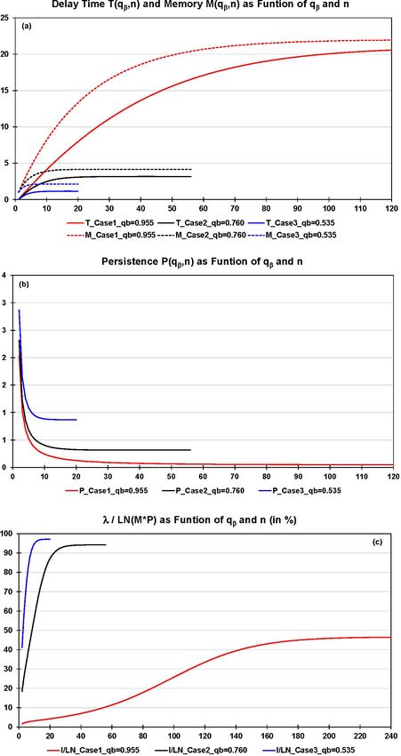
Table 1 shows that the influence of a change in the expo-
fined independently of initial conditions; these only specify
nential growth factor is small vis à vis the dominating influ-
the reference time for n = 0 (here 1959). Figure 7a and b re-
ence of K and D and the quality in the estimates of T , M,
flect the behavior of T , M, and P over time (in units of 1).
and P . For instance, the dimensionless time n at M/M∞ =
For a better overview, Table 1 lists the times when these pa-
0.5 ranges from 15 to 19 in Case 1 and experiments related
rameters exceed 50 % or 95 % of their limiting values (with-
to Case 1 (small persistency) and from 2 to 3 in Case 2 and
out indicating whether these levels go hand in hand with,
experiments related to Case 2 (great persistency); in Case 3
e.g., global-scale ecosystem changes of equal magnitude). In
and experiments related to Case 3, it does not exhibit a range
the table we also specify the ratio λ/ ln(M · P ) for each of
at all (n ≈ 1; very great persistency). These ranges for n tell
these times (see also Fig. 7c). The ratio approaches λ/λβ for
us how long it takes to build up 50 % of the memory with
n → ∞ and indicates (as a percentage) how much smaller the
time running as of n = 0 (1959).
system’s natural rate of change in the numerator turns out to
Alternatively, we can ask how much memory has been
be compared to the system’s rate of change in the denomina-
built up until a given year. Table 2 tells us that after 56 years
tor under the continued increase in stress. As is illustrated, in
(i.e., in 2015) memory is still building up only in Case 1 and
particular by Case 1 in the figure, the ratio does not increase
experiments related to Case 1, which means that the system
at a constant pace as n increases, which shows the nonlinear
still responds in its own characteristic way (as a result of a
strain response of the atmosphere–land and ocean system.
small K and a great D) to the continuously increasing stress;
this is not so in Cases 2 and 3 (and related experiments).
In the latter two cases today’s uptake of carbon by land and
oceans happens de facto outside the system’s natural regime
https://doi.org/10.5194/esd-13-439-2022 Earth Syst. Dynam., 13, 439–455, 2022450 M. Jonas et al.: Quantifying memory and persistence in the atmosphere–land and ocean carbon system
Table 2. Cases 1–3 and related experiments: build-up of mem-
ory (%) as of n = 0 (1959).
Time Increase in memory as of n = 0 (1959)
Cases 1, 12, 13 Cases 2, 21, 23 Cases 3, 31, 32
yr 1 % % %
1959∗ 0 0.0 0.0 0.0
1964 5 17–21 75–76 96
1970 11 34–40 95–96 100
2015 56 88–93 100 –
∗ Start year: σ = ε = 0.
0 0
Finally, it is important to note that it is prudent to expect
that natural elements (like land and oceans) will not con-
tinue to maintain their damping (i.e., carbon uptake) capac-
ity – or their capacity to embark on a, most likely, hysteretic
downward path in the case of a sustained decrease in emis-
sions – even well before they reach the limits of their natural
regimes. They may simply collapse globally when reaching
a critical threshold. We note that our choice of model binds
us to the global scale and also does not allow “failure” to be
specified further, e.g., with respect to when exactly a critical
threshold will occur and in terms of whether carbon uptake
decreases only or even ceases upon reaching the threshold.
To B and C
We report on the sets of stress–strain experiments B and C in
combination. They can be understood as a repetition of the
1959–2015 Case 0 experiment (see A.1) but with the differ-
ence that now upstream emissions as of 1900 (B) or 1850 (C)
are considered. This allows initial conditions for 1959 other
than zero, as in the Case 0 experiment, to be considered (see
Supplement Information 10 and Supplement Data 9 to 16).
Case 0: 1959–2015.
B: 1900–1958 (upstream emissions), 1959–2015.
C: 1850–1958 (upstream emissions), 1959–2015.
Figure 7. Cases 1–3: (a) delay time T and memory M (in units The experiments can be ordered consecutively in terms of
of 1), (b) persistence P (in units of 1), and (c) the ratio λ/ ln(M · P ) time with the three 1959–2015 periods comprising a min–
(in %); all are versus time (in units of 1) as of n = 0 (1959). max interval to facilitate the drawing of a number of robust
results in spite of the uncertainty underlying these stress–
strain experiments (see Supplement Information 10). Be-
and solely in response to the sheer, continuously increasing
tween 1850 and 1959–2015 (i) the compression modulus K
stress imposed on it, whereas in Case 1 and experiments re-
increased from ∼ 2 to 10–13 Pa (the atmosphere became less
lated to Case 1 the limits of the natural regime are not yet
compressible), while (ii) the damping constant D decreased
reached. This interpretation of Cases 1–3 (and related ex-
from ∼ 468 to 459–462 Pa yr (the uptake of carbon by land
periments) does not depend on how much carbon the sys-
and oceans became less viscous), with the consequence that
tem already took up before 1959. M is additive and defined
(iii) the ratio λ = K/D increased from ∼ 0.004–0.005 yr−1
independently of initial conditions; these only specify 1959
to 0.021–0.028 yr−1 (i.e., by a factor of 4–6). Likewise,
as reference time for n = 0. This means by implication that
(iv) delay time T∞ decreased (hence, persistence P∞ in-
the current M value (or its perpetuation) is contained in the
creased) from ∼ 51 (∼ 0.02) to 18–21 (0.047–0.055), while
M value (or is part of that value’s perpetuation) which starts
(v) memory M∞ decreased from ∼ 52 to 19–22 on the di-
accruing from an earlier point in time (see also experiments B
mensionless timescale.
and C below).
Earth Syst. Dynam., 13, 439–455, 2022 https://doi.org/10.5194/esd-13-439-2022M. Jonas et al.: Quantifying memory and persistence in the atmosphere–land and ocean carbon system 451
6 Account of the findings ures globally in the future. These we expect to happen well
before 2050 if the current trend in emissions is not reversed
Here we discuss our main findings in greater depth, recol- immediately and sustainably. However, we reiterate that our
lect the assumptions underlying our global stress–strain ap- choice of model binds us to the global scale and also does
proach, and conclude by returning to the three questions not allow failure to be specified further.
posed at the beginning. We consider our precautionary statement robust given both
We make use of an MB to model the stress–strain behav- the uncertainties we dealt with in the course of our evaluation
ior of the global atmosphere–land and ocean carbon system and the restriction of our variation parameters to two. One of
and to simulate how humankind propelled that global-scale the two variation parameters (λ) presupposes knowing K and
experiment historically, here as of 1850. The stress is given D with equal inaccuracy in relative terms. This procedural
by the CO2 emissions from fossil fuel burning and land use, measure in treating λ, in particular, offers a great applica-
while the strain is given by the expansion of the atmosphere tional benefit but no serious restriction given that (while, ide-
by volume and uptake of CO2 by sinks. The MB is a logi- ally, α is constant) it is the K/D ratio that matters and whose
cal choice of stress–strain model given the uninterrupted in- ultimate value is controlled by consistency – which comes in
crease in atmospheric CO2 concentrations since 1850. as a powerful rectifier. As a matter of fact, fulfilling consis-
The stress–strain model is unique and a valuable adden- tency results in a K/D ratio that ranges close to the lower
dum to the suite of models (such as radiation transfer, en- uncertainty boundary which we deem adequate based on our
ergy balance, or box-type carbon cycle models), which are preceding assessment. That means a smaller K, i.e., the at-
highly reduced but do not compromise complexity in princi- mosphere is more compressible than previously thought, and
ple. These models offer great benefits in safeguarding com- a greater D, i.e., the uptake of carbon by land and oceans is
plex three-dimensional global change models. Here, too, more viscous than previously thought (see Cases 1–3 in Ta-
the proposed stress–strain approach allows three system- ble 1). However, the overall effect of the continued release
characteristic parameters to be distilled from the stress- of CO2 emissions since 1850 on the K/D ratio is unambigu-
explicit equation – delay time, memory, and persistence – and ous – the ratio increased (see λ in Table SI10-2) by a factor
new insights to be gained. What we consider most important of 4–6 (K increased: the atmosphere became less compress-
is that these parameters come with their own internal lim- ible; D decreased: the uptake of carbon by land and oceans
its, which govern the behavior of the atmosphere–land and became less viscous).
ocean carbon system. These limits are independent from any By way of contrast, persistence is less intelligible. Equa-
external target values (such as temperature targets justified tion (5) allows persistence (as well as its systemic limit) to
by means of global change research). be followed quantitatively. However, it is conducive to un-
Knowing these limits is precisely the reason why we can derstand persistence as path dependency and in qualitative
advance the discussion and draw some preliminary conclu- terms, i.e., whether it increased or decreased. Thus, we see
sions. To start with, we look at the Case 0 experiment and that P∞ increased since 1850 by a factor of 2–3 (see P∞ in
the stress–strain experiments B and C in combination. The Table SI10-2), which indicates that the atmosphere–land and
values of the Case 0 parameters T∞ and M∞ , in particular, ocean system is progressively trapped from a path depen-
are at the upper end of the respective 1959–2015 min–max dency perspective. This, in turn, means that it will become
intervals (see Supplement Information 10). That is, the re- progressively more difficult to (strain) relax the entire system
spective characteristic ratios T /T∞ and M/M∞ reach speci- (i.e., the atmosphere including land and oceans) – a mere 1-
fied levels (e.g., 0.5 or 0.95; see Fig. 7a) slightly sooner than year decrease of a few percentage points in CO2 emissions,
when T∞ and M∞ take on values at the lower end of the as reported recently for 2020, will have virtually no impact
1959–2015 min–max intervals. Given that Case 0 is well rep- (Global Carbon Project, 2020).
resented by Case 1, we can use the parameter values of the To conclude, we return to the three questions posed in the
latter. According to column “Case 1” in Table 1, M/M∞ and beginning. These can be answered unambiguously.
T /T∞ reached their 0.5 levels after about 15- and 28-year- Memory, just as persistence, is a characteristic (function)
equivalent units on the dimensionless timescale (which was of the MB. Mathematically spoken, it is contained in the inte-
in 1974 and 1987), whereas they will reach their 0.95 lev- gral on the right side of Eq. (1a) and is defined independently
els after about 64- and 98-year-equivalent units (which will of initial conditions. These appear only in the lower bound-
be in 2023 and 2057) – if the exponential growth factor α ary of that integral, which allows initial conditions other than
remains unchanged in the future. zero to be considered by taking advantage of the integral’s
This not unthinkable worst case provides a reference, as additivity.
follows: we understand, in particular, the ability of a system The memory of the atmosphere–land and ocean carbon
to build up memory effectively as its ability to still respond system – Earth’s memory – can be quantified. It can be un-
to stress in its own characteristic way (i.e., within its nat- derstood as the depreciated strain summed up backward in
ural regime). Therefore, it appears precautionary to prefer time. We let memory extend backward in time to 1850, as-
memory over delay time in avoiding potential system fail- suming zero anthropogenic stress before that date. Memory
https://doi.org/10.5194/esd-13-439-2022 Earth Syst. Dynam., 13, 439–455, 2022You can also read