Quantifying firm-level economic systemic risk from nation-wide supply networks
←
→
Page content transcription
If your browser does not render page correctly, please read the page content below
Quantifying firm-level economic systemic risk from nation-wide supply
                                           networks
                                                       Christian Diema,b , András Borsosa,c,d , Tobias Reische,a , János Kertészd,a , Stefan Thurnere,a,f
                                                       a
                                                         Complexity Science Hub Vienna, Josefstädter Strasse 39, A-1080 Vienna, Austria
                                                       b
                                                         Institute for Finance, Banking and Insurance, Vienna University of Economics and Business, Welthandelsplatz 1,
                                                       A-1080 Vienna, Austria
                                                       c
                                                         Financial Systems Analysis, Central Bank of Hungary
                                                       d
                                                         Department of Network and Data Science, Central European University, Quellenstrasse 51, A-1080 Vienna,
                                                       Austria
                                                       e
                                                         Section for Science of Complex Systems, CeMSIIS, Medical University of Vienna, Spitalgasse 23, A-1090,
                                                       Austria and
                                                       e
                                                         Santa Fe Institute, 1399 Hyde Park Road, Santa Fe, NM 85701, USA∗
arXiv:2104.07260v1 [econ.GN] 15 Apr 2021

                                                       (Dated: April 16, 2021)

                                                       Crises like COVID-19 or the Japanese earthquake in 2011 exposed the fragility of corporate supply
                                                       networks. The production of goods and services is a highly interdependent process and can be
                                                       severely impacted by the default of critical suppliers or customers. While knowing the impact
                                                       of individual companies on national economies is a prerequisite for efficient risk management,
                                                       the quantitative assessment of the involved economic systemic risks (ESR) is hitherto practically
                                                       non-existent, mainly because of a lack of fine-grained data in combination with coherent methods.
                                                       Based on a unique value added tax dataset we derive the detailed production network of an
                                                       entire country and present a novel approach for computing the ESR of all individual firms. We
                                                       demonstrate that a tiny fraction (0.035%) of companies has extraordinarily high systemic risk
                                                       impacting about 23% of the national economic production should any of them default. Firm size
                                                       alone cannot explain the ESR of individual companies; their position in the production networks
                                                       does matter substantially. If companies are ranked according to their economic systemic risk index
                                                       (ESRI), firms with a rank above a characteristic value have very similar ESRI values, while for the
                                                       rest the rank distribution of ESRI decays slowly as a power-law; 99.8% of all companies have an
                                                       impact on less than 1% of the economy. We show that the assessment of ESR is impossible with
                                                       aggregate data as used in traditional Input-Output Economics. We discuss how simple policies of
                                                       introducing supply chain redundancies can reduce ESR of some extremely risky companies.

                                                            Keywords: systemic stability | production networks | shock propagation | cascading failure | network centrality
                                                            measures

                                              Increasing the efficiency of production processes and                   tion processes are highly interdependent. Supplier-buyer
                                           corporate supply chains has been a dominating economic                     relations between companies lead to so-called production
                                           paradigm of the past decades. Popular managerial con-                      networks. The ongoing transformation of production net-
                                           cepts that exemplify this view are reflected in keywords                   works towards higher efficiency has made these networks
                                           such as supply chain management, lean production (Lam-                     more vulnerable to shocks (Craighead et al., 2007). On
                                           ming, 1996), just-in-time delivery (Kannan and Tan,                        regional scales, hurricane Katrina or the Japanese earth-
                                           2005), out- and global sourcing (Hummels et al., 2001;                     quake in 2011 have shown the economic impacts that
                                           Quélin and Duhamel, 2003; Trent and Monczka, 2003), or                    can arise due to subsequent cascading shock propaga-
                                           supply base reduction (Choi and Krause, 2006; Trent and                    tion along corporate supply chains (Carvalho et al., 2020;
                                           Monczka, 1998). Efficiency gains are usually achieved by                   Hallegatte, 2008; Inoue and Todo, 2019). The COVID-19
                                           reducing inventory buffers, shorter lead times, supplier                   pandemic impressively revealed that not only overall eco-
                                           integration, or reducing the number of direct suppliers.                   nomic activity can be affected by interruptions of supply
                                           Actions like these reduce production costs and increase                    chains, but they also may lead to shortages in basic sup-
                                           profits. However, these actions also do have consequences                  plies (Ivanov and Dolgui, 2020), affecting people directly.
                                           in terms of resilience of the overall economy. It has been                 This became apparent, for example, in food production
                                           argued that increased levels of efficiency go hand in hand                 (Bloomberg, 2020), in vaccine supply (The Economist,
                                           with a reduction of resilience (Choi and Krause, 2006;                     2021), computer chips manufacturing, and car manufac-
                                           Craighead et al., 2007).                                                   turing (Financial Times, 2021a,b).
                                             Supply chains of firms and consequently their produc-                       The propagation of shocks through an economy
                                                                                                                      is tightly related to classical input-output economics
                                                                                                                      (Miller and Blair, 2009), where, however, only indus-
                                                                                                                      try sectors are studied. For details and relations to this
                                           ∗ E-mail:   diem@csh.ac.at;   stefan.thurner@muv.ac.at                     work, see Appendix A. The importance of supply chains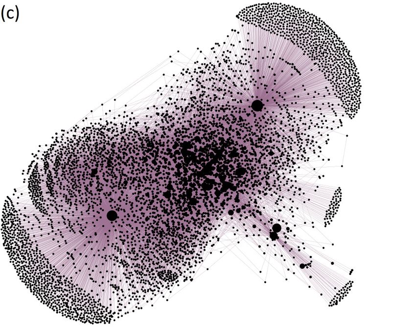
2
at the firm level has been considered by economists, in
particular the consequences of individual company fail-
ure on the overall economy (Acemoglu et al., 2012; Bak
et al., 1993; Gabaix, 2011). The supply chain and pro-
duction management literature studied firm level supply
networks (Choi et al., 2001) and the spreading of disrup-
tions along supply chains under various names, such as
supply chain resilience (Craighead et al., 2007), snowball
effect (Świerczek, 2014), the ripple effect (Ivanov et al.,
2014), or nexus suppliers (Shao et al., 2018). Despite
all these efforts, reliable and systematic estimates of firm
level systemic risk for entire economies are hitherto not
available.
When compared to recent progress in the assessment
of financial systemic risk in financial networks, the quan-
tification of economic systemic risk (ESR) of individual
companies in production networks is still in its infancy.
From initial demonstrations of the relevance of network
structure in the context of financial systemic risk (Allen
and Gale, 2000; Boss et al., 2004a; Elsinger et al., 2006),
by now it is not only possible to assign systemic risk to
individual players in financial networks (Battiston et al.,
2012; Thurner and Poledna, 2013) but also to individ-
ual transactions (Poledna and Thurner, 2016), and on
multiple network layers (Poledna et al., 2015). These de-
velopments allow for novel policy paradigms for systemic
risk regulation (Thurner, forthcoming). To reliably assess
systemic risks detailed and correct information on the
underlying networks is essential (Battiston et al., 2016).
For more information on financial systemic risk and its
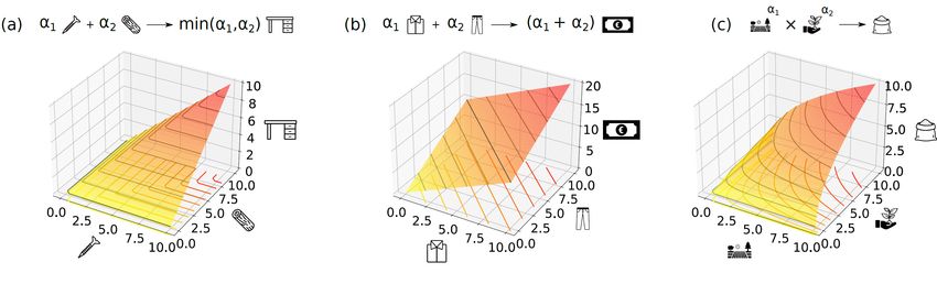
relation to the topic of the present paper, see Appendix FIG. 1 Reconstructing the production network. (a)
B. Schematic supplier-buyer transaction between two companies,
i and j. Supplier i produces product, pi , and delivers a quan-
It is impossible for decision makers to manage eco- tity of Wij to buyer j. The buyer makes a gross payment
nomic systemic risks proactively without understanding consisting of the net price, Vji , and the value added tax, Tji .
which companies pose exceptionally high risk to the en- (b) Production network consisting of eight firms. Color rep-
tire economy in case of their (temporary) failure. It is resents their industry classification. Delivered goods and ser-
therefore important to develop methodology to quantify vices are recorded in the weighted adjacency matrix, where
these risks. Here we show how firm level supply transac- the element Wij (t) records the volume delivered from i to j.
tion data can be used to compute an economic systemic The production function f6 for firm 6 is shown as an example.
risk index (ESRI) for every company within an entire It uses two types of input, p2 = p4 and p7 from firms 2, 4,
and 7 to produce the amount W68 of product p6 . Firm 6 sells
country.
its entire output to firm 8. (c) Section of the Hungarian pro-
The most important ingredient for developing a mean- duction network with 4,070 nodes and 4,845 links. Node size
ingful ESRI is the underlying firm level production net- corresponds to the total strength (proxy for company size).
work, consisting of the supply relations between compa- Many supply “chains” are seen to be connected to form a
nies and their production processes. Country-wide pro- supply network.
duction networks can be reconstructed from firm level
value added tax (VAT) transaction data (Borsos and
Stancsics, 2020; Dhyne et al., 2015)1 . The construction
of the supply network is schematically depicted in FIG. estimate for the volume, Wij , of product type pi , deliv-
1 (a). For every sales transaction between a supplier i ered from supplier i to buyer j. Note that the proxy
and buyer j, the monetary value of the goods and ser- (volume = price × quantity) is a basic assumption in
vices sold, Vji , can be inferred, from the tax rate, τ , and economics (Lequiller and Blades, 2014; Miller and Blair,
the tax amount paid, Tji = τ Vji . We use this as an 2009). For notation, in-links to a node represent sup-
ply transactions (buying); out-links are sales transac-
tions. We define the in-strength
Pn of node i as the sum
of all its in-links, sin
i = j=1 Wji (volume of purchased
1 The value added tax exists in all OECD countries, except for the products),
Pn the out-strength is the sum of all out-links,
USA (OECD, 2020). sout
i = j=1 Wij (sales). The (total) strength is defined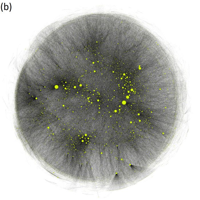
3

as si = sin
          i + si
                out
                    and serves as a proxy for firm-size.        tial in the short term. Note that (Pichler et al., 2020) pro-
   To assess the importance of the supply transaction,          vides a study on which inputs are essential for 56 industry
Wij , between firms i and j, it is essential to know which      sectors. For example, in tire production, rubber interme-
product type, pi , is exchanged and how it is used in the       diates are essential inputs, while consulting services are
production process of firm j. We use the term “prod-            not (short term). The GL treats non-essential inputs in
ucts” for goods and services. Economists typically re-          a linear fashion, while essential inputs are treated in the
sort to the simplifying assumption that every company           non-linear Leontief way. We denote the set of essential in-
produces one out of m different products that is deter-         puts by Iies and non-essential inputs by Iine , respectively.
mined by the company’s industry classification. We use          We define the GL as
                                                                                 "                                    #
an industry affiliation vector, p, that assigns one of m                                h 1     i        1 X
industries to each firm i, pi ∈ {1, 2, . . . , m}. We use              xi = min mines        Πik , βi +            Πik , (1)
                                                                                   k∈Ii  αik            αi
the NACE (Statistical Classification of Economic Activ-                                                         ne
                                                                                                             k∈Ii
ities in the European Community (EUROSTAT, 2021))               where αik are technologically determined coefficients and
classification scheme on the 4-digit level with m = 615         βi is the production level that is possible without non-
categories. For more details on industry classifications,       essential inputs k ∈ Iine ; αi is chosen to interpolate be-
see Appendix C.                                                 tween the full production level (with all inputs) and βi .
   The production process of a company is commonly              Both, α and β, are determined by W , Iies and Iine . Note,
described with a production function (Carvalho and              that we assume labour and capital to be fixed (in the
Tahbaz-Salehi, 2019), fi , that determines the (maximal)        short term) and omit them in the notation. The Leon-
amount of product xi (output) of type pi that firm i            tief production function is a special case of Eq. (1) if
can produce with a given amount of intermediate prod-           all inputs are essential. The linear production function
ucts, Πi = (Πi1 , Πi2 , . . . Πim ) (Πik is the amount of in-   is the special case when all inputs are non-essential; see
put of type k of firm i), its employees (labour), li , and      Appendix D. An essential aspect that determines down-
manufacturing equipment (capital), ci . We use produc-          stream shock propagation is how easily failing suppliers
tion functions that allow us to determine how much firm         can be replaced. For our purposes we assume that com-
i can still produce if a supplier j fails to deliver its        panies with a low market share are easier to replace, than
products of type pj = k to firm i and hence reduces             firms with large market shares; see Appendix E.
the availability of input Πik . This is illustrated with           For the empirical analysis we calibrate the GL in
a small production network in FIG. 1 (b). In-links to           Eq. (1) to four scenarios based on the firms’ NACE
a node (arrows pointing towards node) represent sup-            classifications. First, for a hypothetical purely linear
ply transactions (buying), out-links are sales transac-         production scenario (LIN), all firms have liner produc-
tions. By identifying the supply links belonging to the         tion functions, i.e. only non-essential inputs, or Iine =
inputs in the production function, it can be seen how           {01, . . . , 99}). Second, in a purely Leontief scenario
production depends on the current state of the network.         (LEO), all firms have Leontief functions, i.e. only es-
This is illustrated for firm 6. It uses two types of in-        sential inputs, Iies = {01, . . . , 99}. Third, in a mixed sce-
puts, product a (supplied by firm 2 and 4) and prod-            nario (MIX) we assume all firms within NACE classes
uct b (supplied by firm 7), and produces         an amount     01-45 (physical production) have only essential inputs
x6 (t+1) = f6 W26 (t)+W46 (t), W76 (t) of product c. The        Iies = {01, . . . , 99} and all firms within NACE classes
delivery from 6 to 8, W68 (t+1), depends on the in-links of    46-99 (non-physical production) have only non-essential
6, W68 (t + 1) = f6 W26 (t) + W46 (t), W76 (t) . Should one     inputs Iine = {01, . . . , 99}. Fourth, in the generalized
of the in-links diminish or vanish, this impacts the out-       Leontief scenario (GL) we assume that for firms within
put of 6. This illustrates a so-called downstream shock         NACE 01-45 the set of essential inputs consists of Iies =
propagation of a supply shock. Vice versa, if 8 decides to      {01, . . . , 45} (supplied by physical producers) and the set
no longer buy from 6, the in-links W26 (t), W46 (t), W76 (t)    of non-essential inputs consists of Iine = {46, . . . , 99}
would no longer be needed. This illustrates the upstream        (supplied by non-physical producers), while for firms
propagation of a demand shock.                                  within classes NACE 46-99 we assume they have only
   The specific choice of the production function, fi , de-     non-essential inputs Iine = {01, . . . , 99}. We assume that
termines the intensity of the downstream shock propaga-         firms within NACE 01-45 have a physical production pro-
tion. Frequently used production functions include the          cess while firms within NACE 46-99 predominantly trade
constant elasticity of substitution (CES) (Carvalho et al.,     or provide services. Note that LIN and LEO provide
2020; McFadden, 1963; Moran and Bouchaud, 2019) and             lower and upper bound scenarios for more realistic sit-
its special cases, the Cobb-Douglas (Acemoglu et al.,           uations, where firms have distinct types of production
2012) and the Leontief (Inoue and Todo, 2019; Pichler           functions as in the MIX and GL scenarios.
et al., 2020) production functions, see Appendix D for de-         Given the details of a production network, W , in terms
tails. Here we take a short term perspective and consider       of weighted in-links, out-links, product classification pi ,
a generalized Leontief production function (GL) that ac-        and production functions f , the economic systemic risk
counts for the fact that even for companies with physical       index (ESRI) can finally be computed. It captures the
production processes, not all procured inputs are essen-        consequences of both, the up- and downstream shock
4

propagation following the default of a particular com-          αGL = 0.67 for GL, αMIX = 0.63 for MIX, and αLEO =
pany, i as outlined in Materials and Methods and Ap-            0.50. For details of the fits, see Appendix L, FIG. 7
pendix F and Appendix G. The quantity ESRIi can be              (a). The shape of the rank-ordered ESRI distribution
readily interpreted as the fraction of the production net-      (plateau and power-law tail) is similar to what was found
work’s observed output that is likely to be affected if firm    in Fig 4. in (Moran and Bouchaud, 2019). As expected,
i fails and its output and demand is not replaced by other      the reference case LIN (green) where all companies have
firms. The value is computed by simulating the propa-           linear production functions, generates substantially lower
gation of shocks with the recursive algorithm described         systemic risk levels than GL and MIX. LIN neither shows
in Appendix H.                                                  a plateau nor a power-law decay. The situation is very
                                                                similar in 2016, see FIG. 7 (b) in Appendix L.
                                                                   To better understand which companies are forming the
Results                                                         plateau of extremely risky companies — data protection
                                                                regulations prevent us from showing company names or
   The directed production network W is reconstructed           actual turnover — in FIG. 2 (b) we show ESRIi as a func-
from fully anonymized VAT micro data of the Hungar-             tion of the strength, si (firm size within the network).
ian Central Bank. We consider all links, Wij , where at         Companies on the plateau belong to industry sectors like
least two recurring supply transactions occurred; see Ap-       energy, manufacturing (electrical equipment, chemicals,
pendix I and (Borsos and Stancsics, 2020). Figure 1 (c)         computer and electronics, vehicles), or repair of machin-
shows a section of 4,070 companies and 4,845 links of           ery. Red color indicates the highly risky plateau com-
the empirically reconstructed Hungarian production net-         panies; symbol size represents strength, si . Clearly, the
work, Wij . The section is obtained by sampling 1,500           ESRI of plateau firms (located in the shaded area) is not
random nodes and considering all their direct suppli-           changing with size; in the plateau we find large and small
ers, yielding 6,113 nodes. Only the giant component             companies (note the range of strength of 4 orders of mag-
(4,070 nodes) is shown. The entire network consists of          nitude), suggesting that firm-size is not able to predict
n = 91, 595 companies; it is too large and dense to visual-     extreme ESRI values at all. For the bulk of companies
ize its structure in a meaningful way. Already this small       we find a strong statistically significant correlation of log-
section reveals the fact that production by no means hap-       ESRI and log-strength (R2 = 0.90 and slope βreg = 1.12
pens along independent supply chains, but on a tightly          in log-log regression). However, for individual companies
interwoven complex network. Merged chains that are              strength is not a reliable predictor of ESRI, since the
quite extended are clearly visible. The network has an          spread of the ESRI extends up to 4 orders of magnitude.
apparent core periphery structure. For visualizations of        A more detailed regression analysis, found in Appendix
other aspects of the production network, see Appendix           M, confirms that generally firm level quantities fail to
J.                                                              explain ESRI that is a network-based measure. Note the
   We next calculate the ESRIi for the realistic GL and         relation to the Hulten theorem (Hulten, 1978), stating
MIX scenarios as well as for the two limiting cases, LIN        —in simplified terms— that in an efficient economy the
and LEO for all of the 91, 595 companies in the Hun-            effect of a firm level shock on overall output is propor-
garian VAT micro dataset in the year 2017 and for the           tional to its revenue. Our results are in strong disagree-
85, 131 firms in 2016. Rank-ordered distributions of the        ment with this statement, adding further evidence for its
ESRI are shown in FIG. 2 (a) in linear-log scale for 2017.      limited practical validity (Baqaee and Farhi, 2019). Fi-
For 2016, see FIG. 6 (a) in Appendix K. For the realistic       nally, we checked that all firms on the plateau are within
scenario GL (blue), we find that 32 companies show ex-          NACE 01-45, meaning that their production functions
tremely high levels of systemic risk, all being at a value of   are purely of generalized Leontief type with a large share
about 0.23, meaning that about 23% of the entire econ-          of essential inputs.
omy is affected should one of these companies fail and             The reason for the formation of the plateau is twofold.
its supply and demand is not replaced. 63 and 165 firms         First, about two thirds of its nodes form a strongly con-
have an ESRI larger than 0.05 and 0.01, respectively. For       nected component based on highly critical supplier re-
respective numbers for the other scenarios, see Table I in      lationships (core of plateau). In this core the failure of
Appendix L. The situation is similar for the MIX sce-           one firm leads to the failure of the other members in the
nario, where 47 companies belong to the plateau with            component, implying the default of anyone has the same
values around 0.23. For the (unrealistic) reference case,       consequences on the entire network (same ESRI). The
LEO with all companies of Leontief type (red), for 66           second reason is that the other third of the plateau nodes
firms we find much higher systemic risk levels of about         are suppliers to the strongly connected component, i.e.
0.42.                                                           their failure causes failure of the nodes in the strongly
   For ranks larger than a characteristic rank of 32, the       connected component. These peripheral nodes inherit
pronounced plateau in the distribution is followed first        high ESRI values by supplying (in)directly to inherently
by a steep decline and then by a slow decay of the ESRI         risky companies. Note that these two features are im-
values. The tail (without plateau and steep decline) can        possible to explain with only linear production functions
be fitted to a power-law with an exponent of roughly            (LIN). To illustrate this point, in FIG. 2 (d), we show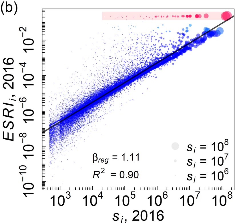
5

                 (a)

                           0.4
                                                              GL
                                                              MIX
                                                              LEO

                    E S R I i 2017
                  0.1 0.2 0.3
                                                              LIN

                           0.0

                                     100 101 102 103 104 105
                                       E S R I i 2017 rank (sorted)

FIG. 2 Economic systemic risk of companies. (a) Economic systemic risk profile (distribution) ESRIi of n = 91, 595 companies
in linear-log scale for 2017. Distributions are rank-ordered, meaning the most risky company is to the very left. The blue line
shows the result for the realistic GL scenario (production functions according to industry classification and classifying produced
goods as essential or not). A plateau exists around an ESRI of 0.23, containing 32 firms for GL. There is a steep decline to
ESRIi ∼ 0.05 from rank 33 to 55. 165 firms have an ESRI larger than 0.01. For comparison the MIX scenario (light blue) is
shown (production functions according to industry classification only). As the limiting cases we show the scenarios LIN (green),
where all firms have linear production functions and LEO (red), where all firms have Leontief production functions. The tail
of the ESRI profile decays as an approximate power-law. (b) ESRI plotted against firm strength (firm-size) in log-log scale.
Symbol size represents strength si , red symbols belong to the plateau, emphasised by the shaded area. We find large and small
companies in the plateau, suggesting that very high ESRI is not determined by size, even though the correlation of ESRI and
strength for the bulk of the companies is high. (c) Systemic risk in 2016 vs. 2017. Colors correspond to ESRI in 2017. Blue
and red symbols indicate low and high values in 2017, respectively. Note the strong variability in the plateau firms. There is
a significant correlation between ESRI in 2017 and 2016, that indicates relatively small temporal fluctuations for the bulk of
the companies. (d) Network of the 32 most systemically risky firms (plateau) in 2017. Node size is proportional to the square
root of strength. Link colors correspond to the downstream ’criticality’, i.e., the percentage of j’s production should i stop
functioning, Λdij . Red thick (blue, thin) links indicate very large (small) losses of production. Small companies predominately
supply to large high-risk companies, thereby inheriting systemic risk.

the network spanned by the 32 plateau firms. Node size                   For systemic risk monitoring of companies it is crucial
                                                √
corresponds to the square root of strength, si ; link col-            to track the change of their systemic riskiness (ESRI)
ors correspond to the direct down-stream impact of the                over time. To estimate the extent of the typical yearly
supplier on the buyer node (criticality), Λdij , (for the defi-       fluctuations, we compare the ESRI values for the years
nition, see Appendix H). Red links indicate highly critical           2016 and 2017 in FIG. 2 (c). Size corresponds to firms’
supplier-buyer relations; Λdij = 1 means that 100% of j’s             log-strength. Of the 68, 254 firms that appear in both
production fails if i fails. Blue links mark non-critical             years, the values of ESRI in 2017 and 2016 are cor-
supplier-buyer relations; Λdij = 0.01 means that j’s pro-             related (ρ(ESRI16 , ESRI17 ) = 0.78, p = 2.2 10−16 ).
duction reduces by 1% if i fails. It is visible that almost           The extent of fluctuations is clearly seen in log-log
all links are critical for the production of the buyer.               representation in FIG. 8 (a) in Appendix N. For the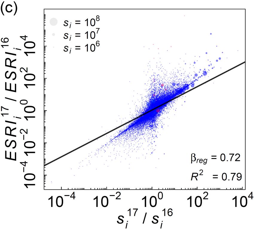
6

logged variables we observe an even higher correlation          and thus systemic risks. As so often in networked dynam-
              16            17
(ρ(log(ESRI) , log(ESRI) ) = 0.85, p = 2.2 10−16 ).             ical systems: details do matter. If studying shocks on the
Figure 8 (c) shows that relative changes in strength ex-        sector level was sufficient, the three scenarios should be
plain the relative changes in ESRI only partially.              strongly correlated. However, the figure suggests that the
   In FIG. 2 (c) temporal changes of companies in the           relative deviations from the sector shock (blue and red
plateau between 2016 and 2017 are seen. The points in           line) are negatively correlated with -19% (p = 5 · 10−6 ).
the horizontal shaded region are those companies in the         In Appendix O we show the actual received shocks (not
plateau in 2017 that had (much) less ESR in 2016. The           their deviations from the reference scenario).
points in the vertical shaded area are those companies             One obvious reason for these large differences between
that are in the plateau in 2016, but not 2017. These            scenarios A and B is made clear in FIG. 3 (b), where
reduced their ESRI. From the 32 plateau companies in            we see for all companies in NACE sector 2611 the in-
2016, 20 remain in the plateau (intersection of shaded          puts at the NACE 4-digit level. Firms (rows) are sorted
regions). Of the 12 companies leaving the plateau from          w.r.t. similarity of their inputs (columns). Even though
2016 to 2017 some remain very risky (light red) others          all companies belong to the same industry sector (NACE
become less risky (blue). 12 companies enter the plateau        2611) the sectors of their inputs vary substantially. The
in 2017 (also firms not contained in the 2016 dataset).         input sectors of Firm A (red shading) and firm B (blue
Possible reasons for these strong fluctuations could be         shading) have only a small overlap, indicated by a Jac-
that core plateau firms added additional suppliers for the      card index of 0.25. Depending on which of two companies
same input, that supply links were discontinued, or that        fails, different input sectors are affected. The Jaccard in-
market share dropped leading to higher supplier replace-        dex for the customer sectors is even smaller (0.13). For
ability. From the data it is hard to decide how these           details on customer sectors, see Appendix O. Among the
factors contribute.                                             51 firms (that in NACE 2611 have NACE 4 classified in-
   To demonstrate that it is necessary to use firm level        puts) 56% have no pairwise input sector overlap (Jaccard
data for any reasonable assessment of shock propaga-            index of zero) and 85% have no pairwise customer sec-
tion in production networks, we compare it to a situation       tor overlap. This means that when choosing two firms
where shocks are studied on a more aggregated level. In         randomly, the probability of having no common input
FIG. 3 (a) we show three different economic shock sce-          (customer) sector is 56% (85%). Consequently, shocks
narios that affect the NACE class 2611 (Manufacture of          to different firms within a sector must lead to different
electronic components). All three initial shocks have the       economic sectors being affected.
same size on the sector level, but affect different compa-
nies within the sector. An initial shock is exogenously
applied and triggers a spreading of shocks in the pro-          Discussion
duction network. The received shock is the shock each
sector receives as a result of the propagation of the ini-         Based on the reconstruction of all relevant buyer-
tial shock. Shock size is measuredPas the fraction of the       supplier relations between companies in an entire coun-
sector’s overall strength, (s2611 = i|pi =2611 si ), affected   try from VAT data, we demonstrate that the real econ-
by the initial shock. The first shock scenario serves as a      omy can not be viewed as a collection of separate supply
reference scenario. It applies a homogeneous initial shock      chains, but is a tightly connected directed network that
of 18% (reduced production) to all of the 69 firms in sec-      has a strongly (weakly) connected component, contain-
tor 2611. The received shock of all (568 NACE 4) sectors        ing 26% (94%) of all companies. The network allows us
(shown on the x-axis) marks the reference response. The         to develop and compute an index for the approximate
received shocks are shown on the y-axis (in log-scale) as       systemic risk of every individual company to the econ-
a fraction of this reference response, and by construc-         omy, ESRI. We demonstrate explicitly that systemic risk
tion, the received shock for the homogeneous scenario is        based on aggregated sector level data yields a severely
1 (black line). In the second scenario a 100% shock (fail-      distorted picture.
ure) is applied to a single firm, A, the received shocks in        We find that the 32 top risky companies contribute to
the different sectors (given as a fraction of the reference     45 % of the entire systemic risk, the top 100 companies
scenario) are shown as the red line. Sectors are sorted         contribute to 74 %. Only 165 companies have more than
w.r.t. received shock sizes in this scenario (A). The third     1% risk. The 32 top risky companies (0.035% of all 91,595
shock scenario applies a 59% shock to firm B, the re-           companies) show extremely high systemic risk of about
sponses are shown by the blue line. Firm A is a plateau         23%. Of those, only a fraction appears to be inherently
firm, firm B is not.                                            risky (e.g., because of size or high market shares). The
   Clearly, the specific choice of the defaulting company       average systemic risk of a Hungarian company is ESRIi =
within the sector has a drastic effect on how the different     0.00018 (mean). The median is 1.7 · 10−6 .
economic sectors are affected. Note that on the sector             Approximately a third of the most risky companies
level the initial shocks are indistinguishable. In other        constitute the periphery of the network of the plateau
words, homogeneous sector shocks (aggregated view)              companies. These are small and inherit systemic risk
yield a grossly false picture of the true shock propagation     from the core plateau companies because they are crit-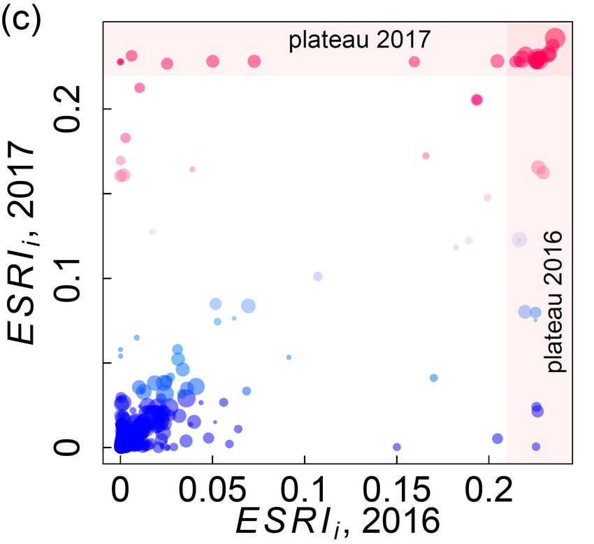
7

                        10−2 10−1 100 101
                 (a)                                                     (b)

                                                                                              70
                     sector−shock deviation

                                                                           Firms of NACE 2611
                                                                                  30    50
                                                shock firm A

                                                                         0 10
                                                shock firm B
                              −3

                                                sector shock
                  10

                                       shock−receiving sector (sorted)                             0       50      100       150
                                                                                                       NACE 4 Class of Inputs
FIG. 3 Importance of firm level analysis. (a) Effect on all 568 NACE 4-digit industry sectors, following a general 18% shock
of the entire NACE sector 2611 (Manufacture of electronic components). The x-axis denotes the 568 shock receiving sectors,
the relative deviation of received shocks from the 18% homogeneous initial shock to sector 2611 is shown on the y-axis. The
black line marks the reference scenario. The red line shows the relative deviation if firm A (in 2611) receives a 100% shock;
the blue line shows the situation for a 59% shock to firm B. Both firm level shocks are equivalent in size to the 18% sector
shock (reference). The particular choice of the defaulting companies lead to drastically different results on how other economic
sectors are affected. (b) Most ubiquitous inputs (at NACE 4 level, columns) for 69 firms (rows) in NACE class 2611. Clearly,
even though all companies belong to the same sector, their input sector vectors are drastically different. Inputs of firm A (red,
50 distinct inputs) and firm B (blue, 49 distinct inputs) differ substantially (Jaccard index 0.25). Note that 18 firms have no
input sectors (empty rows).

ical suppliers to the core. They would not show high                        considered in the algorithm. Its magnitude needs to be
ESRI values if they supplied to other –non-risky– compa-                    estimated in future work and should be taken care of
nies. This means that several of these smaller companies                    in more subtle algorithms. Nonetheless, ours is the first
can be made less risky simply by increasing the number                      attempt to calculate company level ESRI for an entire
of suppliers of the specific good sold to the inherently                    national economy and the resulting index can be seen
risky companies. By analyzing changes of systemic risk                      as a good first-order estimate for the systemic risk in
from 2016 to 2017, we find that ESRI is relatively stable                   production networks. We assume, somewhat unrealisti-
for most companies. However, several smaller companies                      cally, that all customers and all suppliers are treated as
change their ESRI from marginal to extreme, and vice                        being equally important (proportional rationing). Other
versa. The reasons for this might be the risk-inheritance                   rationing mechanisms, for example, prioritizing large cus-
of (non-inherently risky) companies that start (or stop)                    tomers and suppliers, could lead to modified ESRI esti-
supplying to inherently risky ones, or changes in mar-                      mates. For a detailed discussion of the effects of rationing
ket shares that affect their replaceability. We confirmed                   mechanisms at the sector level, see (Pichler and Farmer,
that to a large extent systemic risk is not predictable                     2021). Further, for the implementation of the algorithm
with strength (firm-size). The position in the supply net-                  we assumed a data-driven replaceability index for each
work matters much more than company-size, similarly to                      firm that is based on its market share (fraction of out-
what has been observed in financial systemic risk in ear-                   put within its NACE 4 class). This implies that firms
lier studies (Battiston et al., 2012; Markose et al., 2012;                 with high (low) market shares are difficult (easy) to re-
Thurner and Poledna, 2013).                                                 place, see Appendix E. Further improvement of the ESRI
                                                                            would be possible by modelling the substitutability of in-
   The presented study has limitations. The proposed                        puts and the replaceability of suppliers in more detail.
measure is an economically motivated, straightforward                       However, this comes with the cost of more parameters
quantitative measure for systemic relevance of compa-                       to calibrate, more detailed data needs, and significantly
nies in a given production network. It captures up- and                     higher computational effort.
down-stream impacts independently. This doesn’t cause
distortions in tree-like supply chains, however, in net-                       For assigning production functions to companies, we
works with strongly connected components it does. In                        used a simple matching based on NACE 2-digit cate-
reality, the same firm can be affected by up- and down-                     gories. Although we think that this is a good first ap-
stream shocks; these shocks can potentially interact. For                   proximation, we emphasize that this can be a source of
example, the lack of a critical input (down-stream shock)                   error. Given the current data availability, an exact and
can translate into an upstream shock for suppliers of                       objective mapping of production functions to companies
complementary inputs. This second-order effect is not                       is not feasible. Large-scale firm level surveys providing
8
information on how strongly firms are affected by the lack of the financial sector, risk concentration can be avoided
of specific inputs could be a useful first step clarifying this by demanding that no customer should have more than
point. a certain supply exposure (e.g. 10% of total exposure).
We assume a static production network, which in re- Inventory buffers. A natural possibility is to intro-
ality, is a temporal network. With this simplification, duce mandatory inventory buffers for systemically risky
seasonality effects in production and manufacturing are companies, to ensure production in situations where a set
missed. Also, in the present implementation we don’t of critical suppliers default.
consider competition between companies that would re- Make economic systemic risk visible for firms.
sult in a dynamic restructuring of the network. Moreover, Today, companies usually manage their direct suppliers.
it is technically hard to interpret the time index t in terms Most companies do not know their higher-order depen-
of how long shocks really need to spread and converge. dencies in the production network (GEODIS, 2017). It
For simplicity, we assume uniform spreading, i.e. all pe- is conceivable that it could be highly beneficial to many
riods t are of the same abstract length. Imports, exports, producing companies to obtain a better overview on their
and production networks of other countries are not con- actual supply and customer risks. If countries provided
sidered due to lack of data. This is a limitation since a more global view on supply chains to identify critical
Hungary is a small, open economy with significant expo- situations, this could lead to deeper and more proactive
sures to shocks in the global economy. In principle the systemic supply chain management, that would increase
vulnerability to initial shocks from import and export re- overall economic resilience by using market mechanisms.
lationships can be considered in our framework by using Policies and regulatory measures of this kind might
coarse grained sector level import-export information. run contrary to the hunt for efficiency that dominated
Despite these limitations, our findings have a number the last decades, since supplier relations are time- and
of policy implications. cost intensive. More resilience does not pay off in the
Monitoring. The economic systemic risk index for short term. It would be a fascinating question to see
individual companies, ESRI, allows countries to use VAT to what extent the economy could be made more re-
tax data to identify critical companies in the economy silient by not making it less efficient, i.e. to maximize
and their critical supply relations (via their marginal the resilience-gain per link. For financial networks the
ESRI contributions, see (Poledna and Thurner, 2016)). potential of designing networks with lower systemic risk,
Our findings indicate that only a few firms pose a sub- but comparable economic function was recently high-
stantial risk to the overall economy. These should be lighted in (Diem et al., 2020; Pichler et al., 2021). A
monitored closely if they produce goods of societal rel- related question is whether service-based economies are
evance. In particular, sharp increases in firms’ systemic more resilient than production-based ones because ser-
riskiness can be monitored over time. Several countries vices typically require less critical suppliers (due to their
are currently implementing “supply chain due diligence” linear production functions). Instead of asking whether
laws, for example, Germany (Financial Times, 2021c) or large economies are more stable than small ones (Moran
the USA (Biden, 2021). The possibilities for systemic and Bouchaud, 2019), our methodology, given data from
risk monitoring as presented in this paper should be kept other countries, could contribute to the question, whether
in mind, when designing new regulation. production-based economies or economies with high lev-
Systemic risk mitigation. A straightforward way els of input-redundancy are more resilient.
to increase resilience in the real economy is to introduce
supply chain redundancies, where risk is reduced by al-
tering the network structure and thereby reducing the
probability for inherently systemically risky firms to suf- Material and Methods
fer failures that result from a lack of inputs. We have
shown that a simple network analysis allows us to identify The economic systemic risk index for firm i is calcu-
the inherently risky firms. For those, contingency plans lated as
should be established to buy time for changing suppliers
n
or to build alternative production capacities. The change sout
Pn j out 1 − hj (T )
X
of ESRI over time would allow countries to monitor if im- ESRIi = , (2)
j=1 l=1 sl
plemented policies really increase resilience levels of the
economy.
x (T )
Avoiding risk concentration. In (Poledna and where hj (T ) = xjj (0) is the fraction of the output remain-
Thurner, 2016) it has been shown how incentive schemes ing of firm j at time T , where T is the convergence time,
can be designed to make financial networks safer without see Appendix F. ESRIi , is interpreted as the fraction of
making them less efficient. A similar scheme could be de- output that is lost in the entire production network in re-
vised for production networks by de-incentivizing critical sponse to the failure of individual company i, given that
supply relations. A simple scheme would be to have at its supply and demand can not be replaced. The vector
least one back-up supplier for every critical product that h(T ) = min(hd (T ), hu (T )) is the result of propagating
is shipped to inherently risky firms. Like in regulations the shock from firm i’s initial default downstream along9
the out-links by updating Borsos, A., and M. Stancsics, 2020, Unfolding the hidden
n
structure of the Hungarian multi-layer firm network, Tech-
X nical Report, Magyar Nemzeti Bank (Central Bank of Hun-
xdl (t + 1) = fj Wji hdj (t)δpj ,1 , . . . , (3) gary).
j=1
! Boss, M., H. Elsinger, M. Summer, and S. T. 4, 2004a,
n
X Quantitative Finance 4(6), 677, URL https://www.
Wji hdj (t)δpj ,m , tandfonline.com/doi/abs/10.1080/14697680400020325.
j=1 Boss, M., M. Summer, and S. Thurner, 2004b, in Interna-
tional Conference on Computational Science (Springer),
and upstream along the in-links by updating pp. 1070–1077.
n
X Carvalho, V. M., 2014, Journal of Economic Perspectives
xul (t + 1) = Wlj huj (t) . (4) 28(4), 23, URL https://www.aeaweb.org/articles?id=
j=1 10.1257/jep.28.4.23.
Carvalho, V. M., M. Nirei, Y. U. Saito, and A. Tahbaz-
For details of the calibration to the GL, see Appendix F, Salehi, 2020, The Quarterly Journal of Economics 136(2),
Appendix G, for the implementation, see Appendix H. 1255, ISSN 0033-5533, URL https://doi.org/10.1093/
qje/qjaa044.
Carvalho, V. M., and A. Tahbaz-Salehi, 2019, Annual Review
References of Economics 11(1), 635, URL https://doi.org/10.1146/
annurev-economics-080218-030212.
Acemoglu, D., V. M. Carvalho, A. Ozdaglar, and A. Tahbaz- Choi, T. Y., K. J. Dooley, and M. Rungtusanatham,
Salehi, 2012, Econometrica 80(5), 1977, URL https:// 2001, Journal of Operations Management 19(3), 351,
onlinelibrary.wiley.com/doi/abs/10.3982/ECTA9623. ISSN 0272-6963, URL https://www.sciencedirect.com/
Allen, F., and D. Gale, 2000, Journal of Political Economy science/article/pii/S0272696300000681.
108(1), 1. Choi, T. Y., and D. R. Krause, 2006, Journal of Oper-
Arinaminpathy, N., S. Kapadia, and R. M. May, 2012, Pro- ations Management 24(5), 637, ISSN 0272-6963, URL
ceedings of the National Academy of Sciences 109(45), https://www.sciencedirect.com/science/article/
18338, ISSN 0027-8424, URL https://www.pnas.org/ pii/S0272696305001233.
content/109/45/18338. Clauset, A., C. R. Shalizi, and M. E. J. Newman, 2009,
Atalay, E., A. Hortacsu, J. Roberts, and C. Syverson, SIAM Review 51(4), 661, URL https://doi.org/10.
2011, Proceedings of the National Academy of Sciences 1137/070710111.
108(13), 5199, ISSN 0027-8424, URL https://www.pnas. Colon, C., S. Hallegatte, and J. Rozenberg, 2021, Nature Sus-
org/content/108/13/5199. tainability 4(3), 209.
Bak, P., K. Chen, J. Scheinkman, and M. Wood- Cont, R., A. Moussa, and E. Santos, 2010, SSRN,
ford, 1993, Ricerche Economiche 47(1), 3, ISSN 0035- doi:10.2139/ssrn.1733528 .
5054, URL https://www.sciencedirect.com/science/ Craighead, C. W., J. Blackhurst, M. J. Rungtusanatham,
article/pii/003550549390023V. and R. B. Handfield, 2007, Decision Sciences 38(1),
Baqaee, D. R., and E. Farhi, 2019, Econometrica 87(4), 131, URL https://onlinelibrary.wiley.com/doi/abs/
1155, URL https://onlinelibrary.wiley.com/doi/abs/ 10.1111/j.1540-5915.2007.00151.x.
10.3982/ECTA15202. Dhyne, E., G. Magerman, and S. Rubı́nová, 2015, The Belgian
Bardoscia, M., S. Battiston, F. Caccioli, and G. Caldarelli, production network 2002-2012, Technical Report, NBB
2015, PLOS ONE 10(7), e0130406. Working Paper.
Barrot, J.-N., and J. Sauvagnat, 2016, The Quarterly Journal Diem, C., A. Pichler, and S. Thurner, 2020, Journal of Eco-
of Economics 131(3), 1543, ISSN 0033-5533, URL https: nomic Dynamics and Control 116, 103900, ISSN 0165-
//doi.org/10.1093/qje/qjw018. 1889, URL https://www.sciencedirect.com/science/
Battiston, S., G. Caldarelli, R. M. May, T. Roukny, and article/pii/S0165188920300683.
J. E. Stiglitz, 2016, Proceedings of the National Academy Douglas, P. H., 1976, Journal of Political Economy 84(5),
of Sciences 113(36), 10031, ISSN 0027-8424, URL https: 903, URL https://doi.org/10.1086/260489.
//www.pnas.org/content/113/36/10031. Eisenberg, L., and T. H. Noe, 2001, Management Science
Battiston, S., M. Puliga, R. Kaushik, P. Tasca, and G. Cal- 47(2), 236, URL https://doi.org/10.1287/mnsc.47.2.
darelli, 2012, Scientific Reports 2(541). 236.9835.
Beale, N., D. G. Rand, H. Battey, K. Croxson, R. M. May, and Elsinger, H., A. Lehar, and M. Summer, 2006, Manage-
M. A. Nowak, 2011, Proceedings of the National Academy ment Science 52(9), 1301, URL https://doi.org/10.
of Sciences 108(31), 12647, ISSN 0027-8424, URL https: 1287/mnsc.1060.0531.
//www.pnas.org/content/108/31/12647. EUROSTAT, 2021, Your companion guide to interna-
Biden, J. R., 2021, Executive order on america’s sup- tional statistical classifications. section iv - description
ply chains, URL https://www.whitehouse.gov/ of the main economic classifications, URL https:
briefing-room/presidential-actions/2021/02/24/ //ec.europa.eu/eurostat/ramon/miscellaneous/
executive-order-on-americas-supply-chains/. index.cfm?TargetUrl=DSP_GENINFO_CLASS_4.
Bloomberg, 2020, Meat-Shortage Risk Climbs with Financial Times, 2021a, Chip shortage forces audi to
25% of U.S. Pork Capacity Offline, URL https: delay production, URL https://www.ft.com/content/
//www.bloomberg.com/news/articles/2020-04-22/ 8cb74f6a-3859-4b13-885e-0e79a4d5de1a.
tyson-foods-to-indefinitely-suspend-waterloo/ Financial Times, 2021b, Ford says chip shortage could
operations-k9bbgnr9. knock $2.5bn from earnings, URL https://www.ft.com/10 content/a0d5ca20-2559-4d47-9106-cf50eaf97720. McFadden, D., 1963, The Review of Economic Studies 30(2), Financial Times, 2021c, German cabinet backs 73, ISSN 00346527, 1467937X, URL http://www.jstor. law to protect human rights in global sup- org/stable/2295804. ply chain, URL https://www.ft.com/content/ Miller, R. E., and P. D. Blair, 2009, Input-Output Analysis: 2b969d2c-ad1e-48c2-b318-2dd20bb1662f. Foundations and Extensions (Cambridge University Press). Freixas, X., B. M. Parigi, and J. C. Rochet, 2000, Journal of Moran, J., and J.-P. Bouchaud, 2019, Phys. Rev. E Money, Credit and Banking 32(3), 611. 100, 032307, URL https://link.aps.org/doi/10.1103/ Furfine, C. H., 2003, Journal of Money, Credit and Banking PhysRevE.100.032307. 35(1), 111, ISSN 00222879, 15384616, URL http://www. Nier, E., J. Yang, T. Yorulmazer, and A. Alentorn, 2007, jstor.org/stable/3649847. Journal of Economic Dynamics and Control 31(6), 2033. Gabaix, X., 2011, Econometrica 79(3), 733, URL https:// OECD, 2020, Consumption Tax Trends 2020 (OECD onlinelibrary.wiley.com/doi/abs/10.3982/ECTA8769. Paris), URL https://www.oecd-ilibrary.org/content/ Gai, P., and S. Kapadia, 2010, Proceedings of the Royal So- publication/152def2d-en. ciety A: Mathematical, Physical and Engineering Sciences Pichler, A., and J. D. Farmer, 2021, Modeling simultaneous 466(2120), 2401. supply and demand shocks in input-output networks. GEODIS, 2017, SUPPLY CHAIN WORLDWIDE Pichler, A., M. Pangallo, R. M. del Rio-Chanona, F. Lafond, SURVEY, Technical Report, GEODIS, URL and J. D. Farmer, 2020, Production Networks and Epi- https://geodis.com/sites/default/files/2019-03/ demic Spreading: How to Restart the UK Economy? 170509_GEODIS_WHITE-PAPER.PDF. Pichler, A., S. Poledna, and S. Thurner, 2021, Jour- Giannetti, M., M. Burkart, and T. Ellingsen, 2011, The Re- nal of Financial Stability 52, 100809, ISSN 1572- view of Financial Studies 24(4), 1261, ISSN 0893-9454, 3089, URL https://www.sciencedirect.com/science/ URL https://doi.org/10.1093/rfs/hhn096. article/pii/S1572308920301121. Hallegatte, S., 2008, Risk Analysis: An International Jour- Poledna, S., J. L. Molina-Borboa, S. Martı́nez-Jaramillo, nal 28(3), 779, URL https://onlinelibrary.wiley.com/ M. van der Leij, and S. Thurner, 2015, Journal of doi/abs/10.1111/j.1539-6924.2008.01046.x. Financial Stability 20, 70, ISSN 1572-3089, URL Hanel, R., B. Corominas-Murtra, B. Liu, and S. Thurner, https://www.sciencedirect.com/science/article/ 2017, PloS one 12(2), e0170920. pii/S1572308915000856. Hulten, C. R., 1978, The Review of Economic Studies 45(3), Poledna, S., and S. Thurner, 2016, Quantitative Finance 511, ISSN 00346527, 1467937X, URL http://www.jstor. 16(10), 1599. org/stable/2297252. Quélin, B., and F. Duhamel, 2003, European Man- Hummels, D., J. Ishii, and K.-M. Yi, 2001, Jour- agement Journal 21(5), 647, ISSN 0263-2373, URL nal of International Economics 54(1), 75, ISSN 0022- https://www.sciencedirect.com/science/article/ 1996, URL https://www.sciencedirect.com/science/ pii/S0263237303001130. article/pii/S0022199600000933. Rauch, J. E., 1999, Journal of International Economics 48(1), Inoue, H., and Y. Todo, 2019, Nature Sustainability 2(9), 841. 7, ISSN 0022-1996, URL https://www.sciencedirect. Ivanov, D., and A. Dolgui, 2020, International Journal of Pro- com/science/article/pii/S0022199698000099. duction Research 58(10), 2904, URL https://doi.org/ Shao, B. B., Z. M. Shi, T. Y. Choi, and S. Chae, 10.1080/00207543.2020.1750727. 2018, Decision Support Systems 114, 37, ISSN 0167- Ivanov, D., B. Sokolov, and A. Dolgui, 2014, International 9236, URL https://www.sciencedirect.com/science/ Journal of Production Research 52(7), 2154, URL https: article/pii/S0167923618301374. //doi.org/10.1080/00207543.2013.858836. The Economist, 2021, How vaccines are made, and Kannan, V. R., and K. C. Tan, 2005, Omega 33(2), 153, why it is hard, URL https://www.economist. ISSN 0305-0483, URL https://www.sciencedirect.com/ com/science-and-technology/2021/02/06/ science/article/pii/S030504830400060X. how-vaccines-are-made-and-why-it-is-hard. Lamming, R., 1996, International Journal of Operations & Thurner, S., forthcoming, A Complex Systems Perspective on Production Management 16(2), 183, URL https://doi. Macroprudential Regulation. org/10.1108/01443579610109910. Thurner, S., and S. Poledna, 2013, Scientific Reports 3, 1888. Leontief, W., 1928, Archiv fur Sozialwissenschaft und Trent, R. J., and R. M. Monczka, 1998, International Sozialpolitik 60, 577. Journal of Purchasing and Materials Management 34(3), Leontief, W., 1991, Structural Change and Eco- 2, URL https://onlinelibrary.wiley.com/doi/abs/10. nomic Dynamics 2(1), 181, ISSN 0954-349X, URL 1111/j.1745-493X.1998.tb00296.x. https://www.sciencedirect.com/science/article/ Trent, R. J., and R. M. Monczka, 2003, International Journal pii/0954349X9190012H. of Physical Distribution & Logistics Management 33(7), Lequiller, F., and D. Blades, 2014, Understanding 607. National Accounts (OECD Paris), URL https: Varian, H. R., 2014, Intermediate Microeconomics: A Mod- //www.oecd-ilibrary.org/content/publication/ ern Approach: Ninth International Student Edition (WW 9789264214637-en. Norton & Company). Magerman, G., K. De Bruyne, E. Dhyne, and J. Van Hove, Wu, D., 2016, Essays on the interface between finance and 2016, Heterogeneous firms and the micro origins of aggre- technology. gate fluctuations, Technical Report, NBB Working Paper. Świerczek, A., 2014, International Journal of Production Markose, S., S. Giansante, and A. R. Shaghaghi, 2012, Jour- Economics 157, 89, ISSN 0925-5273, the Interna- nal of Economic Behavior & Organization 83(3), 627, tional Society for Inventory Research, 2012, URL ISSN 0167-2681, URL https://www.sciencedirect.com/ https://www.sciencedirect.com/science/article/ science/article/pii/S0167268112001254. pii/S0925527313003654.
11

Acknowledgments

  This work was supported in part by the OeNB
Hochschuljubiläumsfund P17795 the Austrian Science
Promotion Agency FFG under 857136, the Austrian
Science Fund FWF under P29252, H2020 SoBigData-
PlusPlus grant agreement ID 871042.
12

Appendix A: Relation to I-O analysis

   On the industry level studies on the propagation of shocks in production networks exist at least since the famous
Leontief Input-Output analysis (Leontief, 1928, 1991; Miller and Blair, 2009). In (Bak et al., 1993) it is shown
theoretically that small shocks to individual sectors can have effects on aggregate output. Refs. (Acemoglu et al.,
2012; Carvalho, 2014; Gabaix, 2011) confirm this finding. (Hallegatte, 2008) assess higher order shocks from the
Hurricane Katrina disaster. More recently, (Pichler et al., 2020) investigated how demand and supply constraints on
the sector level affect GDP. In (Colon et al., 2021) it is modeled how shocks spread through the Tanzanian supply
and transport network. The sector level analysis produced valuable insights, but it has certain limitations due to the
nature of the underlying data. Only recently high-quality large-scale firm level data has become available that allows
for new insights.
   The methodology presented in this paper addresses three usual shortcomings of sector level analyses. First, the data
shows that even within fine grained industry classifications (NACE 4) firms tend to have considerably heterogeneous
input sectors and customer sectors. In fact when comparing the pairwise input (customer) sectors of firms we see that
for all firms in NACE 2611 (Manufacture of electronic components) 56% (85%) have no overlap of input (customer)
sectors even though they belong to the same NACE 4 category, see FIG. 3 in the main text and Appendix O. Second,
this intra-sector heterogeneity can lead to inaccurate results when using them for assessing shock propagation in
production networks. Especially if the initial crises scenario does not affect all firms within a sector to the same
extent (for example in the current COVID-19 crises). Our proposed framework takes this into account and yields
different cascades for shocks which would appear to be the same at industry level, but are actually distributed
heterogeneously among firms within an industry. FIG. 3 (a) shows in a simple example how two cascades that are the
same on the industry level lead to very different impacts on other firms and industry sectors. Third, in contrast to
sector level models, each firm in our approach has a specific production function based on its industry classification
that is calibrated to the observed individual input vector of the respective firm; see Appendix D for more information
on the calibration of production functions. This matters especially since we show in FIG. 3 (b) that firm input vectors,
even in the fine grained industry classifications, vary on the sector level. The same is shown for customer sectors, see
Appendix O, FIG. 9 (b).
   Since, data has become available also firm level analysis has been performed. Ref. (Atalay et al., 2011) uses a gen-
erative model for firm level production networks that matches degree distributions better than scale-free frameworks.
Belgian VAT data has been used to study productivity shocks to individual firms and their effects on aggregate output
with a computeable equilibrium model (Magerman et al., 2016). The theoretical study (Moran and Bouchaud, 2019)
shows that shocks propagate widely as soon as production function have a “Leontief” component, but not when they
are of pure Cobb-Douglas type. Probably the closest study to ours, (Inoue and Todo, 2019), investigates how firm
level shock propagation in response to an initial shock –the great earthquake in Japan in 2011– based on an estimate
of the Japanese production network. However, they focus on effects on aggregate output and do not compute firm
level systemic risk.

Appendix B: Relations to financial systemic risk

   In the area of financial networks systemic risk has been extensively studied for about two decades (Boss et al.,
2004a; Freixas et al., 2000). The importance of being able to measure systemic risk of single firms (banks, insurance,
funds) became apparent in the 2008 financial crises and the European government debt crises 2012. Initial systemic
risk assessment methodologies have been shown by, for example, (Boss et al., 2004b; Eisenberg and Noe, 2001;
Furfine, 2003) they have been refined to macroprudential stresstesting models that can assess the effects of adverse
macro-economic scenarios (Elsinger et al., 2006) and to measure the impact single banks have on the entire network
(Battiston et al., 2012; Cont et al., 2010). A wide range of studies revealed various properties of financial networks
that improve the understanding of how systemic risk emerges, for example, the role of network topology (Gai and
Kapadia, 2010; Nier et al., 2007), the role of diversification of external assets (Beale et al., 2011), or the role played by
large banks (Arinaminpathy et al., 2012). These aspects are crucial for the management of systemic risk. The design
of regulatory policies to address the adverse economic and societal effects of systemic risk has strongly benefited from
these academic contributions. However, there are important differences between financial and production networks
and how stress is spreading there, that require adaptions to how systemic risk and the spreading of shocks is defined
and modelled. For example, in production networks in- and out-links affect heterogeneous production process in
contrast to stock quantities like equity or liquidity buffers in financial networks. Further, production networks tend to
be orders of magnitude larger than banking networks. Here we extent the ideas of measuring systemic risk in financial
networks (Bardoscia et al., 2015; Battiston et al., 2012; Cont et al., 2010) to a more general framework of companies
in a production network at a national scale. To estimate it we use micro level VAT data of Hungary (Borsos and
You can also read