Prediction and Prevention of Pandemics via Graphical Model Inference and Convex Programming
←
→
Page content transcription
If your browser does not render page correctly, please read the page content below
Prediction and Prevention of Pandemics
                                                           via Graphical Model Inference and Convex Programming
                                        Mikhail Krechetov1 , Amir Mohammad Esmaieeli Sikaroudi2 , Alon Efrat2,3 , Valentin Polishchuk4 ,
                                                                       and Michael Chertkov3,5,2,1
                                                                   1
                                                                     Skolkovo Institute of Science and Technology, Moscow, Russia, 121205
                                                             2
                                                               Department of Computer Science, University of Arizona, Tucson, AZ, USA, 85721
                                                             3
                                                               Program in Applied Mathematics, University of Arizona, Tucson, AZ, USA, 85721
                                                                             4
                                                                               Linkoping Univeristy, Norrkoping, Sweden, 60174
                                                                5
                                                                  Department of Mathematics, University of Arizona, Tucson, AZ, USA, 85721
                                                                           Mikhail.Krechetov@skoltech.ru, chertkov@arizona.edu
arXiv:2109.04517v1 [cs.SI] 9 Sep 2021

                                                                  Abstract                                  Introduction: Graphical Models of Pandemics
                                                                                                            We follow our previous work (Chertkov et al. 2021) in jus-
                                                                                                            tification for the use of the Graphical Models (GM) to study
                                        Hard-to-predict bursts of COVID-19 pandemic revealed sig-           and mitigate pandemics. Therefore, we start from providing
                                        nificance of statistical modeling which would resolve spatio-       a brief recap of the prior literature on modeling of the epi-
                                        temporal correlations over geographical areas, for example          demics, describe the logic which led us in (Chertkov et al.
                                        spread of the infection over a city with census tract granu-        2021) to the Ising Model (IM) formulation, and then state
                                        larity. In this manuscript, we provide algorithmic answers to       formally the inference and prevention problems addressed
                                        the following two inter-related public health challenges of         in the manuscript.
                                        immense social impact which have not been adequately
                                        addressed by the AI community. (1) Inference Challenge:                 Difficulty in both predicting and neutralizing the spread
                                        assuming that there are N census blocks (nodes) in the city,        of pandemics is a major social challenge of humanity. Tech-
                                        and given an initial infection at any set of nodes, e.g. any N of   nically speaking, we are yet to design a coherent data lifecy-
                                        possible single node infections, any N (N − 1)/2 of possible        cle for modeling and prevention both in terms of the global
                                        two node infections, etc, what is the probability for a subset      strategies and local tactics. To address the challenge, we
                                        of census blocks to become infected by the time the spread of       must devise a hierarchy of spatio-temporal models with dif-
                                        the infection burst is stabilized? (2) Prevention Challenge:        ferent resolutions – from individual to community, county
                                        What is the minimal control action one can take to minimize         to the city, and from the moment a pathogen first enters our
                                        the infected part of the stabilized state footprint? To answer      bodies, to days of disease development and to community
                                        the challenges, we build a Graphical Model of pandemic of
                                                                                                            transmission. Importantly, the models should be efficient in
                                        the attractive Ising (pair-wise, binary) type, where each node
                                        represents a census track and each edge factor represents the       computing probabilistic predictions (for instance, offering
                                        strength of the pairwise interaction between a pair of nodes,       the marginal probability heat map for the city neighborhoods
                                        e.g. representing the inter-node travel, road closure and re-       to transition from the current/prior state of infection to the
                                        lated, and each local bias/field represents the community level     projected/a-posteriori state in two weeks).
                                        of immunization, acceptance of the social distance and mask             Epidemiology and Mathematical Biology experts have
                                        wearing practice, etc. Resolving the Inference Challenge re-        relied in the past on a number of modeling approaches.
                                        quires finding the Maximum-A-Posteriory (MAP), i.e. most            The Agent-Based-Models (ABMs), introduced in epidemi-
                                        probable, state of the Ising Model constrained to the set of        ology in 2004-2008 (Eubank et al. 2004; Longini et al.
                                        initially infected nodes. (An infected node is in the +1 state
                                        and a node which remained safe is in the −1 state.) We show
                                                                                                            2005; Ferguson et al. 2005, 2006; Germann et al. 2006;
                                        that almost all attractive Ising Models on dense graphs result      Halloran et al. 2008), have complemented the earlier com-
                                        in either of the two possibilities (modes) for the MAP state:       partmental models (Ross 1910; Kermack, McKendrick, and
                                        either all nodes which were not infected initially became in-       Walker 1927; Anderson and May 1991; Hethcote 2000).
                                        fected, or all the initially uninfected nodes remain uninfected     Using ABMs, even though not exclusive to epidemiology
                                        (susceptible). This bi-modal solution of the Inference Chal-        (Wikipedia 2020; Downey 2018), became a breakthrough
                                        lenge allows us to re-state the Prevention Challenge as the         in the field, as they allowed to make a significant improve-
                                        following tractable convex programming: for the bare Ising          ment in the quality of predictions, especially in the spatio-
                                        Model with pair-wise and bias factors representing the system       temporal resolution of how the disease spreads and how
                                        without prevention measures, such that the MAP state is fully       one can mitigate its spread. The models became and re-
                                        infected for at least one of the initial infection patterns, find
                                        the closest, in l1 norm, therefore prevention-optimal, set of
                                                                                                            mained a core part of the epidemiology data life-cycle. (See
                                        factors resulting in all the MAP states of the Ising model, with    for instance (Lovasi and et.al. 2020; Kerr et al. 2021) for
                                        the optimal prevention measures applied, to become safe.            most recent bibliography.) The ABMs provide a detailed
                                                                                                            prediction of how pandemics spread within counties, cities,
                                                                                                            and regions. A majority of the country-, city- or county-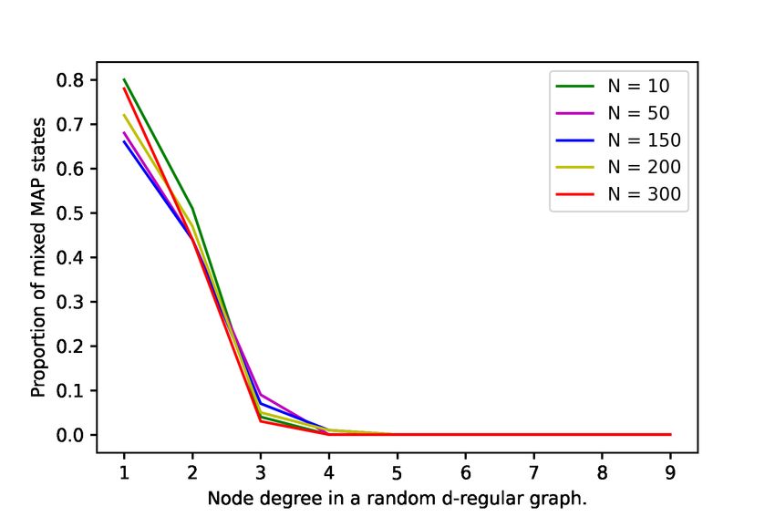
scale testbeds testing various mitigation strategies are re-      cubation period. If an infected person enters a communi-
solved nowadays with ABMs. In particular, recently ABMs           ty/neighborhood but does not stay there, he infects others
have been used extensively to inform public health in (non-       with some probability. If a single resident of the commu-
pharmaceutical) interventions against the spread of COVID-        nity becomes infected, all other residents are assumed in-
19 (Ferguson et al. 2020; Eubank et al. 2020; LANL 2020;          fected as well (instantaneously). The model is a discrete-
Maziarz and Zach 2020; Kaxiras and Neofotistos 2020), and         time dynamic model in which nodes in a network are in one
verify new strategies like test-trace-quarantine (Kerr et al.     of the three states: Susceptible, Infected, or Removed. The
2021), among many other applications.                             nodes represent communities/neighborhoods. A contact be-
   There are two major problems with the modeling of pan-         tween an Infected community/node and another community
demic. First, many parameters need to be calibrated on data.      which is Susceptible has an assigned probability of disease
Second, even when calibrated for the current state of pan-        transmission, which can also be interpreted as the probabil-
demic the models which are too detailed become impractical        ity of turning the S state into I state. Consistently with what
for making a forecast and for developing prevention strate-       was described above, the network is represented as a graph,
gies – both requiring checking multiple (forecast and/or pre-     where nodes are tracts and edges, connecting two tracts,
vention) scenarios. Using ABMs, which are clearly over-           have an associated strength of interaction representing the
modeled (too detailed) is especially problematic in the con-      probability for the infection to spread from one node to its
text of the latter. For example, the open-source ABM solver       neighbor. A seed of the infection is injected initially at ran-
FLUTE (Chao et al. 2010) developed originally for model-          dom, for example, mimicking an exogenous super-spreader
ing influenza, works with data that are acquired through Ge-      infection event in the area; examples could include political
ographic Information Systems (GIS) on the scale of census         or religious gatherings. See Figure 1 illustrating dynamics
tracts or communities, which is a very reasonable scale of        of the cascade model over 3-by-3 grid graph. Color cod-
spatial resolution to understand the dynamics of pandemics        ing of nodes is according to Susceptible=blue, Infected=red,
on a local scale. FLUTE populates each of the communi-            Removed=black. Given the starting infection configuration,
ties with thousands to millions of inhabitants in order to        each infected community can infect its graph-neighbor com-
account for their daily patterns of travel. We believe that       munity during the next time step with the probability as-
constructing effective Graphical Models (GM) of Pandemics         sociated with the edge connecting the two communities.
with community-scale spatial resolution and then model-           Then the infected community moves into the removed state.
ing pairwise (and possibly higher-order) epidemic interac-        The attempt to infect each neighbor is independent of all
tions between communities directly, without introducing the       other neighbors. This creates a cascading spread of the virus
thousands-to-millions of dummy agents, will complement            across the network. The cascade stops in a finite number of
(as discussed in the next paragraph), but also improve upon       steps, thereby generating a random Removed pattern, shown
ABMs by being more efficient, robust and easier to calibrate.     in black in the Fig. 1, while other communities which were
   An important, and possibly one of the first, Graphical         never infected (remain Susceptible) are shown in blue.
Model (GM) of the COVID-19 pandemic was proposed in                  It was shown in (Chertkov et al. 2021) that with some
(Chang et al. 2020). Dynamic bi-partite GMs connecting            regularization applied, statistics of the terminal state of the
census tracts to specific Points Of Interest (non-residential     Cascade Model of Pandemic turns into a Graphical Model
locations that people visit such as restaurants, grocery stores   of the attractive Ising Model type.
and religious establishments) within the city and studying           This manuscript Road Map. Working with the Ising
dynamics of the four-state (Susceptible, Exposed, Infectious      Model of Pandemic, we start the technical part of the
and Removed) of a census tract (graph node) on the graph,         manuscript by posing the Inference/Prediction Challenge
were constructed in (Chang et al. 2020) for major metro-area      in Section 1. Here, the problem is stated, first, as the Max-
in USA based on the SafeGraph mobility data (SafeGraph            imum A-Posteriori over an attractive Ising Model, and we
2021).                                                            argue, following the approach which is classic in the GM
   In fact, similar dynamic GMs, e.g. of the Independent          literature, that problem can be re-stated as a tractable LP.
Cascade Model (ICM) type (Kempe, Kleinberg, and Tar-              We then proceed to Section 2 to pose the main challenge ad-
dos 2003; Netrapalli and Sanghavi 2012; Gomez-Rodriguez,          dressed in the manuscript – the Prevention Challenge – as
Leskovec, and Krause 2012; Khalil, Dilkina, and Song 2013;        the two-level optimization with inner step requiring resolu-
Rosenfeld, Nitzan, and Globerson 2016), were introduced           tion of the aforementioned Prediction Challenge. Aiming to
even earlier in the CS/AI literature in the context of mod-       reduce the complexity of the Prevention problem, we turn in
eling how the rumors spread over social networks (with a          Section 3 to the analysis of the conditions in the formulation
side reference on using ICM in epidemiology). As argued           of the Prediction Challenge, describing the Safety domain
in (Chertkov et al. 2021) the Independent Cascade Mod-            in the space of the Ising Model parameters. We show the
els (ICMs) can be adapted to modeling pandemics. (An-             Safety domain is actually a polytope, even though exponen-
other interesting use of the ICM to model COVID-19 pan-           tial in the size of the system. We proceed in Section 5 with
demic was discussed in (Chen et al. 2020).) In its mini-          analysis of the Prevention Challenge, discussing the inter-
mal version, an ICM of Pandemic can be built as follows.          pretation of the problem as a projection to the Safety Poly-
Assume that the virus spreads in the community (census            tope from the polytope exterior, needed when the bare pre-
tract) sufficiently fast, say within five days – which is the     diction suggests that system will be found with high proba-
estimate for the early versions of COVID-19 median in-            bility outside of the Safety Polytope. Section 4 is devoted to
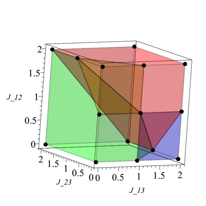
Figure 1: An exemplary random sequence (top-left to top-right to bottom-left to bottom-right) of the Independent Cascade
Model (ICM) dynamics over 3 × 3 grid. Nodes colored red, blue, and black are Infected, Susceptible, and Removed at the
respective stage of the dynamical process. This (shown) sample of the dynamic process terminates in 3 steps. Ising Model of
Pandemic (IMP), which is the focal point of this manuscript, describes a regularized version of the ICM terminal state, where
only two states (S-blue and R-black) are left. (See text for details.)
approximation which allows an enormous reduction in the where we emphasize dependence of the MAP solution on
problem complexity. We suggest here that if the graph of the the set of the initially infected nodes, I.
system is sufficiently dense, the resulting MAP solution may Note that in general finding x(MAP) is NP-hard (Barahona
only be in one of the two polarized states (a) completely safe 1982). However if J > 0 element-wise, i.e. the Ising Model
(no other nodes except the initially infected) pick the infec- is attractive (also called ferromagnetic in statistical physics),
tion, or (b) the infection is spread over the entire system. We Eq. (4) becomes equivalent to a tractable (polynomial in N )
support this remarkable simplification by detailed empirical Linear Programming (see (Živný, Werner, and Průša 2014)
analysis and also by some theoretical arguments. Section 6 is and references therein). In fact, the IMP is attractive, reflect-
devoted to the experimental illustration of the methodology ing the fact that the state of a node is likely to be aligned
on the practical example of the Graphical Model of Seattle. with the state of its neighbor.
The manuscript is concluded in Section 7 with a brief sum- Let us also emphasize some other features of the IMP:
mary and discussion of the path forward.
1. G should be thought of as an ”interaction” graph of a city,
reflecting transportation, commutes, and other forms of
1 Ising Model of Pandemic interactions between populations with the homes at the
As argued in (Chertkov et al. 2021) the terminal state of a two nodes (census tracts) linked by an edge. The strength
dynamic model generalizing the ICM model can be repre- of a particular Jab shows the level of interaction associ-
sented by the Ising Model of Pandemic (IMP), defined over ated with the edge {a, b}.
graph G = (V, E), where V is the set of N = |V| nodes and
E is the set of undirected edges. The IMP, parameterized by 2. A component, ha , of the vector of local biases, h, is
the vector of the node-local biases, h = (ha |a ∈ V) ∈ RN , reflecting a-node specific factors such as immunization
and by the vector of the pair-wise (edge) interactions, J = level, imposed quarantine, and degree of compliance
(Jab |{a, b} ∈ E), describes the following Gibbs-like proba- with the public health measures (e.g., wearing masks and
following other rules). Large negative/positive ha shows
bility distribution for a state, x = (xa = ±1|a ∈ V) ∈ 2|V| , that residents of the census tract associated with the node
associated with V: a are largely healthy/infected.
exp (−E(x | J, h))
P (x | J, h) = , (1) If solution of the Inference Challenge problem is such that
Z(J, h)
the R-subset of the MAP solution, x(MAP) (I|J, h), i.e.
where any node, a ∈ V can be found in either S- (suscept-
able, never infected) state, marked as xa = −1, or R- (re-
n o
R(I, J, h) = a ∈ V | x(MAP)
a (I|J, h) = +1 , (5)
moved, i.e. infected prior to the termination) state, marked
as xa = +1. In Eq. (1), E(x|J, h) and Z(J, h) are model’s is sufficiently large, we would like to mitigate the infection,
energy function and partition function respectively: therefore setting the Prevention Challenge discussed in the
X X
E(x | J, h) = ha xa − Jab xa xb , (2) next Section.
a∈V a,b∈V
2 Prevention Challenge
Let us assume that modification of J and h are possible and
X X X
Z(J, h) = ha xa − Jab xa xb .(3)
x a∈V a,b∈V
consider the space of all feasible J and h. We will then iden-
tify Safe Domain as a sub-space of feasible J and h such that
In what follows, we will focus on finding the Maximum- for all the initial sets of the initially infected nodes, I, con-
A-Posteriori (MAP) state of the IMP conditioned to a par- sidered the resulting ”infected” subset, R(I, J, h), is suffi-
ticular initialization – setting a subset of nodes, I ∈ V, to be ciently small. A more accurate definition of the Safe Domain
infected. We coin the MAP problem Inference Challenge: follows. Then, we rely on the definition to formulate the
x(MAP) (I|J, h) = arg min E(x | J, h) , (4) control/mitigation problem coined Prevention Challenge. At
x ∀a∈I: xa =+1 this stage, we would also like to emphasize that studying thegeometry of the Safe Domain is one of the key contributions E(x(j) | J, h), which is linear in (J, h). For a subset, R ⊆ V,
of this manuscript. of nodes, let x(R) be the state in which, xa = +1, ∀a ∈
Definition. Consider IMP over G = (V, E) and with the R, xa = −1, ∀a ∈ / R. Let X (R) be the set of all the MAP
parameters (J, h). Let us also assume that the set of initially states, x, such that ∀a ∈ R, xa = +1 (while other nodes,
infected nodes, I, is drawn from the list, Υ. We say that i.e. b ∈ V \ R, are not constrained, xb = ±1). Then the
(J, h) is in the k-Safe Domain if for every I from Υ the k-Safe Polytope, which we denote, SP(k), is defined by at
number of R-nodes in the MAP solution (4), is at most k, k
N N −k0
P
i.e. most k0 · (2 − 1) linear inequalities:
k0 =1
∀I ∈ Υ : |R(I, J, h)| ≤ k, (6) \n o
SP(k) = (J, h) | E(x(R) |J, h) > E(x | J, h) ,
where R(I, J, h) is defined in Eq. (5). ∀R, |R| ≤ k;
Prevention Challenge: Given (J (0) , h(0) ) describing the ∀x ∈ X (R) \ x(R)
bare status of the system (city) which is not in the k-
(8)
Safe Domain, and given the cost of the (J, h) change,
were some of these linear inequalities on the rand hand side
C (J, h); (J (0) , h(0) ) , what is least expensive change to may be redundant.
(J (0) , h(0) ) state of the system which is in the the k-Safe Remark. In the case of k = 1 (which, obviously, ap-
Domain? Formally, we are interested to solve the following plies only if all the initial infections are at a single nodes,
optimization: i.e. ∀I ∈ Υ, |I| = 1), there are at most, N · (2N −1 − 1)
linear inequalities.
(J (corr) , h(corr) ) = arg min C (J, h); (J (0) , h(0) ) . We illustrate the geometry of the Ising model over the tri-
(J,h) Eq. (6)
angle graph (three nodes connected in a loop, K3 ) in Fig. 2
(7)
and Fig. 3. For both illustrations, we fix the h value to −1
Expressing it informally, the Prevention Challenge seeks at all the nodes, and we are thus exploring the remaining
to identify a minimal correction (thus ”corr” as the upper in- three degrees of freedom, J12 , J13 , J23 (since J is symmet-
dex) (J (corr) , h(corr) ), which will move the system to the safe ric), which corresponds to exploring interactions within the
regime from the unsafe bare one, (J (0) , h(0) ). The measures class of attractive Ising models, ∀a, b = 1, 2, 3 : Jab ∈ R+ .
may include limiting interaction along some edges of the First, we consider the case when the only node
graph, thus modifying some components of J, or enforcing a = 1 is infected. In this simple setting there
local biases, e.g., increasing level of vaccination, at some are four possible MAP states, (x1 , x2 , x3 ) ∈
component of h. {(+1, −1, −1), (+1, −1, +1), (+1, +1, −1), (+1, +1, +1)},
Given that condition in Eq. (6) also requires solving shown in Fig. (2) as green, blue, yellow and red, respec-
Eq. (4) for each candidate (J, h), the Prevention Challenge tively. Finally, in the figure Fig. (3) we plot the Safe
formulation is a difficult two-level optimization. However, Polytope SP(1). We observe that the two ”polarized” MAP
as we will see in the next Section, the condition in Eq. (6) states, (+1, −1, −1) and (+1, +1, +1), are seen most often
(and thus the inner part of the aforementioned two-level op- among the samples, while domain occupied by the other
timization) can be re-stated as the requirement of being in- two ”mixed” MAP states, (+1, −1, +1) and (+1, +1, −1)
side of a polytope in the (J, h) space. In other words, the is much smaller, with the two modes positioned on the
(k)-Safe Domain is actually a polytope in the (J, h) space. interface between the two polarized states.
As will be shown below in the next Section, the polar-
ization phenomena with only two ”polarized” MAP states,
3 Geometry of the MAP States which we coin in the following the two polarized modes,
Before solving the Prevention Challenge problem, we want which we see on this simple triangle example, is generic for
to shed some light on the geometry of the MAP states. We the attractive Ising model.
work here in the space of all the Ising models over a graph
G = (V, E), where each of the models is specified by (J, h). 4 Two Polarized Modes
Proposition. Safe Domain of a graph G = (V, E) with
Definition. Consider a particular subset of the initially in-
N = |V| nodes is a polytope in the space of all feasible
fected nodes, I (where thus, ∀a ∈ I : xa = +1). We
parameters, (J, h), defined by an exponential in N number
call the MAP state of the model polarized when one of the
of linear constraints.
following is true: (i) only initially infected nodes show +1
Remark. The Proposition allows us, from now on, to use within the MAP solution, ∀a ∈ I : xa = +1, ∀b ∈ V \ I :
Safe Polytope instead of the Safe Domain. xb = −1 or (ii) all nodes within the MAP state show +1,
Proof of the Proposition. The space of all the Ising mod- ∀a ∈ V : xa = +1. We call a MAP state mixed otherwise.
els is divided into 2N regions by the corresponding MAP Experimenting with many dense graphs, which are typ-
states. Moreover, the boundary between any pair of neigh- ical in the pandemic modeling of modern cities with ex-
boring regions is linear: consider two states x(i) and x(j) , tended infrastructures and multiple destinations visited by
and denote (J, h)(i) (resp. (J, h)(j) ) the set of all the Ising many inhabitants, we observe that the two polarized MAP
models with the MAP state x(i) (resp. x(j) ), then (J, h)(i) states dominate generically, while the mixed states are ex-
and (J, h)(j) are separated by the equation, E(x(i) | J, h) = tremely rare.Figure 2: Geometry of the attractive Ising model illustrated Figure 3: The Safe Polytope illustrated on the example of a
on the example of a triangle graph (K3 ) when a single node triangle graph (K3 ) with field vector h = [−1, −1, −1]. See
is infected. See explanations in the text. explanations in the text.
We will continue discussion of the two-mode solution in
Fig. 4 illustrates results of one our ensemble of random the next Section.
IMPs’ experiments. We, first, fix N to 20, pick M such that
M ≤ N (N − 1)/2 = 190 and then generate at random M
edges connecting the 20 nodes. Then, for each of the ran-
5 Projecting to the Safe Polytope
dom graphs (characterized by its own M ) we generate 500 In this Section we aim to summarize all the findings so far
random samples of (J, h), representing attractive Ising mod- to resolve the Prevention Challenge formulated in Section 2,
els. Finally, we find the MAP state for each IMP instance, specifically in Eq. (7) stating the problem as finding a mini-
count the number of mixed states and show the dependence mal projection to the Safety Domain/Polytope from its exte-
of the fractions of the mixed states (in the sample set) in the rior. The task is well defined, but in general, and as shown in
Fig. (4). A fast decrease of the proportion of the mixed states Section 3, it is too complex – as the description of the Safety
is observed with an increase in M . Polytope (number of linear constraints, required to define it)
is exponential in the system size (number of nodes in the
Extension of these experiments (see Fig. (5)) suggests that
graph). However, the two-mode approximation, introduced
when we consider an ensemble of IMPs over graphs with N
in Section 4, suggests a path forward: use the two-mode ap-
nodes and the average degree α = O(1) which is sufficiently
proximation and therefore remove all the linear constraints
large (so that the graph is sufficiently dense) and increase
but one, separating the two polarized states.
N , we observe that the Mixed State Probability (MSP), or
Let us denote the two-mode approximation of the Safe
equivalently proportion of the mixed-to-polarized states, de-
creases dramatically. Moreover, based on the experiments, Polytope by SPd(Υ), where thus k in the original Safe Poly-
we conjecture that the MSP decays to zero at α > αc , but it tope, SP (k), is replaced by the set Υ of all the initial infec-
saturates at α < αc , where αc is the threshold depending on tion patters. Then we write,
the ensemble details. This threshold behavior is akin to the \
phase transition that occurred in many models of the spin SP
d(Υ) = (J, h) | E(+12N | J, h) ≥ E(x(I) | J, h) ,
I∈Υ
glass theory (Mezard, Parisi, and Virasoro 1986) and many
models of the Computer Science and Theoretical Engineer- (9)
ing defined over random graphs and considered in the ther- (I) (I)
modynamic limit, i.e. at N → ∞. See e.g. (Richardson and where, ∀a ∈ I : xa = +1 and ∀b ∈ V \ I : xb = −1.
Urbanke 2008) (application in the Information Theory, and Eq. (9) represents a polytope stated in terms of the |Υ| con-
specifically in the theory of the Low Density Parity Check straints. In particular, if Υ accounts for all the initial infec-
Pk
tions, I, of size not large than k, then |Υ| = k0 =1 kN0 : the
Codes) (Mezard and Montanari 2009) (applications in the
Computer Science, and specifically for random SAT and re- number of constraints grows exponentially in the maximal
lated models) and references therein. We postpone further size of the initial infections, however the number of the con-
discussions of the conjecture for a future publication (see straints remains tractable for any k = O(1). Replacing con-
also brief discussion in Section 7). ditions in Eq. (7) by SP
d(Υ), defined in Eq. (9), one arrives atFigure 4: Proportion of the mixed states in all samples for an Figure 5: Proportion of the mixed-to-polarized states for an
ensemble of the (attractive) Ising Model of Pandemic over ensemble of the (attractive) Ising Model of Pandemic over d-
graphs with N nodes, shown as a function of the varying regular graphs with N nodes, shown as a function of d. Each
number of edges, M . Each shown point is the result of the point is the result of averaging over 100 random instances of
averaging over 500 random instances of the (J, h) over the the (J, h) over different random graphs with the same node
same graph. (See text for additional details.) degree. (See text for additional details.)
the following tractable (in the case of k = O(1)) convex op- This results in the estimation of the pair-wise interactions,
timization expression answering the Prevention Challenge J, parameterizing the Ising Model of Pandemic. We also
approximately (within the two-mode approximation): come up with an exemplary (uniform over the system) lo-
cal biases, h, completing the definition of the model. (We
(Jb(corr) , b
h(corr) ) = arg min C (J, h); (J (0) , h(0) ) . remind that the prime focus of the manuscript is on devel-
(J,h) Eq. (9)
(10) oping methodology which is AI sound and sufficiently gen-
eral. Therefore, the data used in the manuscript are roughly
This formula is the final result of this manuscript analytic representative of the situation of interest, however not fully
evaluation. In the next Section we use Eq. (10), with C(·; ·) practical.) We consider a situation with different levels of in-
substituted by the l1 -norm, to present the result of our ex- fection and chose (J (0) , h(0) ) stressed enough, that is result-
periments in a quasi-realistic setting describing a (hypothet- ing in the prediction (answer to our Prediction Challenge),
ical) pandemic attack and optimal defense, i.e., prevention which lands the system in the dangerous domain – outside
scheme. of the Safety Polytope.
6 Experiments Convex projection
Seattle data In all of our experiments, we have used the general-
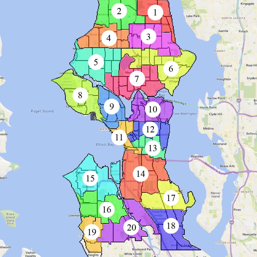
We illustrate our methodology on a case study of the city of purpose Gurobi optimization solver (Gurobi Optimization,
Seattle. Seattle has 131 Census Tracts. (Each Census Tract LLC 2021) to compute the MAP states and thus to validate
includes 1 to 10 Census Block Groups with 600 to 3000 res- the two-mode assumption. (We have also experimented with
idents.) Each Census Tract represents 1200 to 8000 popula- CVXPY (CVXPY 2021), but found it performing slower
tion, and its boundaries are designed to represent natural or than Gurobi, at least over the relatively small samples con-
urban landmarks and also to be persistent over a long period sidered in this proof of principles study. In the future, we
(United States Census Bureau 2019). To reduce complex- plan to use existing, or developing new, LP solvers de-
ity, we merge census tracts into 20 regions. See Fig. 6. To signed specifically for finding the MAP state of the attrac-
prepare this splitting of Seattle into 20 regions/nodes, we tive Ising model.) To illustrate our Prevention strategy, we
utilize geo-spatial information from the TIGER/Line Shape- took the Seattle data described above, and fed it as an in-
files project provided by U.S. Census Bureau (United States put into the optimization (10), describing projection to the
Census Bureau 2021). The travel data of Seattle was ex- Safety Polytope, where C(·; ·) is substituted by the l1 norm.
tracted from the Safegraph dataset (Saf), which provides CVXPY solver was used for this convex optimization task.
anonymized mobile tracking data. Each data point in the Our code (python within jupyter notebook) is available at
Safegraph database describes the number of visits from a https://github.com/mkrechetov/IsingMitigation.
Census Block to a specific point of interest represented by Table 1 shows results of our Prevention experiments on
latitude and longitude. Mobility data associated with travel- the Seattle data. We analyze l1 projection to SP d(Υ) where
ers crossing the boundaries of Seattle was ignored. We then Υ consists of all the initial infection patterns consisting of up
follow the methodology developed in (Chertkov et al. 2021) to k nodes. In all of our experiments, the values of the field
to combine the aggregated travel data with the epidemiolog- vector h (uniform across the system) was fixed to −1. We
ical data, representing current state of infection in the area. observe that the number of constraints grows exponentiallyprobability of significant infection is above a pre-defined (by
the public health experts) tolerance threshold. We show that
in its simplest formulation, the prevention problem is equiv-
alent to finding minimal l1 projection to the safety polytope,
where the latter is defined by solving the aforementioned
prediction problem. In general, the polytope does not allow a
description non-exponential in the size of the system. How-
ever, we suggested an approximation that allows to approx-
imate the safety polytope efficiently - that is, linearly in the
number of the initial infection patterns. The approximation
is justified (empirically, with supporting theoretical argu-
ments, however not yet backed by a mathematically rigorous
theory) in the case when the interaction graph of the system
(e.g., related to the system/city transportation and human-
to-human interaction network) is sufficiently dense. We con-
clude by providing a quasi-realistic experimental demonstra-
tion on the GM of Seattle.
We conclude the manuscript with an incomplete list of
AI challenges, presented in the order of importance (subjec-
tive), which need to be resolved to make the powerful GM
Figure 6: Seattle case study areas and census tracts (Office approach to pandemic prediction and prevention practical:
of Planning & Community Development, Seattle 2010). • Build a hierarchy of Probabilistic Graphical Models
which allow more accurate (than Ising model) represen-
k LP Constraints Runtime Cost tation of the infection patterns over geographical and
1 801 1.65s 41.69 community graphs. The models may be both of the
2 991 3.04s 43.62 static (like Ising) or dynamic (like Independent Cascade
3 2131 10.90s 44.30 Model) types. Extend the notion of the Safety Region
4 6976 100.08s 44.56 (polytope) to the new GM of pandemics.
• Consider the case when the resolution of the Prediction
Table 1: Summary of our prevention experiments on the Challenge problem returns a positive answer - most likely
Seattle data. k, in the first column, is the maximal number of future state of the system is safe, and then develop the
nodes in the initially infected patterns (all accounted for to methodology which allows estimating the probability of
construct the k-Safe Polytope). The second column shows crossing the safety boundary. In other words, we envi-
number of linear constraints characterizing the k-Safe Poly- sion formulating and solving in the context of the GM
tope. Respective Run Time and Cost are shown in the 3rd a problem which is akin to the one addressed in (Owen,
and 4th column, where Cost shows the difference in l1 norm Maximov, and Chertkov 2019): estimate the probability
between the (J (0) , h(0) ), characterizing stressed but unmit- of finding the system outside of the Safety Polytope.
igated regime, and the optimal prevention regime, resulting • Construct other (than two-mode) approximations to the
in (Jb(corr) , b
h(corr) ) computed according to Eq. (10). Safety Polytope. Approximations built on sampling of
the boundaries of the safety polytope and learning (pos-
sibly reinforcement learning) are needed.
with k; however, the cost of intervention remains roughly • Develop the asymptotic (thermodynamic limit) theory
the same. We intend to analyze the results of this and other which allows validating (and/or correcting systemati-
(more realistic) experiments in future publications aimed at cally) the efficient (two-mode and other) approximations
epidemiology experts and public health officials. of the Safety Polytope.
7 Conclusions and Path Forward Acknowlegments
In this manuscript, written specifically for the AI com- This work was supported in part by NSF via #2027072
munity, we follow our prior work (Chertkov et al. 2021), ”RAPID:Infer and Control Global Spread of Corona-Virus
aimed at a broader interdisciplinary community, and explain with Graphical Models” project.
respective inference (prediction) and control (prevention)
questions/challenges. We use the language of GMs, which
is one powerful tool in the modern arsenal of AI, and state
the Prediction Challenge as a MAP optimization over an at-
tractive Ising model, which can be expressed generically as
a solution of a tractable Linear Programming (LP). We then
turn to the analysis of the prevention problem, which is set
if the aforementioned prediction solution suggests that theReferences Germann, T. C.; Kadau, K.; Longini, I. M.; and Macken,
???? SafeGraph COVID-19 Data Consortium. San Fran- C. A. 2006. Mitigation strategies for pandemic influenza in
cisco, CA: SafeGraph Inc. the United States. Proceedings of the National Academy of
Anderson, R.; and May, R. 1991. Infectious Disease of Hu- Sciences, 103(15): 5935–5940.
mans: Dynamics and Control. Oxford University Press, Ox- Gomez-Rodriguez, M.; Leskovec, J.; and Krause, A. 2012.
ford. Inferring Networks of Diffusion and Influence. ACM Trans.
Barahona, F. 1982. On the computational complexity of Knowl. Discov. Data, 5(4).
Ising spin glass models. Journal of Physics A: Mathemat- Gurobi Optimization, LLC. 2021. Gurobi Optimizer Refer-
ical and General, 15(10): 3241–3253. ence Manual. https://www.gurobi.com.
Chang, S.; Pierson, E.; Koh, P. W.; Gerardin, J.; Redbird, B.; Halloran, M. E.; Ferguson, N. M.; Eubank, S.; Longini,
Grusky, D.; and Leskovec, J. 2020. Mobility network mod- I. M.; Cummings, D. A. T.; Lewis, B.; Xu, S.; Fraser, C.;
els of COVID-19 explain inequities and inform reopening. Vullikanti, A.; Germann, T. C.; Wagener, D.; Beckman, R.;
Nature. Kadau, K.; Barrett, C.; Macken, C. A.; Burke, D. S.; and
Chao, D. L.; Halloran, M. E.; Obenchain, V. J.; and Cooley, P. 2008. Modeling targeted layered containment of
Longini Jr, I. M. 2010. FluTE, a publicly available stochas- an influenza pandemic in the United States. Proceedings of
tic influenza epidemic simulation model. PLoS Comput Biol, the National Academy of Sciences, 105(12): 4639–4644.
6(1): e1000656. Hethcote, H. W. 2000. The Mathematics of Infectious Dis-
Chen, Y.-C.; Lu, P.-E.; Chang, C.-S.; and Liu, T.-H. 2020. eases. SIAM Rev., 42(4): 599–653.
A Time-Dependent SIR Model for COVID-19 With Unde- Kaxiras, E.; and Neofotistos, G. 2020. Multiple Epidemic
tectable Infected Persons. IEEE Transactions on Network Wave Model of the COVID-19 Pandemic: Modeling Study.
Science and Engineering, 7(4): 3279–3294. Journal of Medical Internet Research, 22(7): e20912.
Chertkov, M.; Abrams, R.; Esmaieeli Sikaroudi, A. M.; Kempe, D.; Kleinberg, J.; and Tardos, E. 2003. Maximizing
Krechetov, M.; Slagle, C.; Efrat, A.; Fulek, R.; and Oren, Y. the Spread of Influence through a Social Network. In Pro-
2021. Graphical Models of Pandemic. https://www.medrxiv. ceedings of the Ninth ACM SIGKDD International Confer-
org/content/10.1101/2021.02.24.21252390v1.full. ence on Knowledge Discovery and Data Mining, KDD ’03,
CVXPY. 2021. Convex Optimization for Everyone. https: 137–146. New York, NY, USA: Association for Computing
//www.cvxpy.org/. Machinery. ISBN 1581137370.
Downey, A. 2018. Think Complexity: Complexity Science Kermack, W. O.; McKendrick, A. G.; and Walker, G. T.
and Computational Modeling. O’Reilly Media, Inc., 2nd 1927. A contribution to the mathematical theory of epi-
edition. ISBN 1549761749. demics. Proceedings of the Royal Society of London. Se-
Eubank, S.; Eckstrand, I.; Lewis, B.; Venkatramanan, S.; ries A, Containing Papers of a Mathematical and Physical
Marathe, M.; and Barrett, C. L. 2020. Commentary on Fer- Character, 115(772): 700–721.
guson, et al., “Impact of Non-pharmaceutical Interventions Kerr, C. C.; Stuart, R. M.; Mistry, D.; Abeysuriya, R. G.;
(NPIs) to Reduce COVID-19 Mortality and Healthcare De- Rosenfeld, K.; Hart, G. R.; Nunez, R. C.; Cohen, J. A.; Sel-
mand”. Bulletin of Mathematical Biology, 82(4): 52. varaj, P.; Hagedorn, B.; George, L.; Jastrzebski, M.; Izzo,
Eubank, S.; Guclu, H.; Anil Kumar, V. S.; Marathe, M. V.; A. S.; Fowler, G.; Palmer, A.; Delport, D.; Scott, N.; Kelly,
Srinivasan, A.; Toroczkai, Z.; and Wang, N. 2004. Mod- S. L.; Bennette, C. S.; Wagner, B. G.; Chang, S. T.; Oron,
elling disease outbreaks in realistic urban social networks. A. P.; Wenger, E. A.; Panovska-Griffiths, J.; Famulare, M.;
Nature, 429(6988): 180–184. and Klein, D. J. 2021. Covasim: An agent-based model of
COVID-19 dynamics and interventions. PLOS Computa-
Ferguson, N.; Laydon, D.; Nedjati-Gilani, G.; Imai, N.;
tional Biology, 17(7): 1–32.
Ainslie, K.; Baguelin, M.; Bhatia, S.; Boonyasiri, A.;
Cucunubá, Z. M.; Cuomo-Dannenburg, G.; Dighe, A.; Khalil, E. B.; Dilkina, B.; and Song, L. 2013. CuttingEdge:
Dorigatti, I.; Fu, H.; Gaythorpe, K.; Green, W.; Hamlet, Influence minimization in networks. In Workshop on Fron-
A.; Hinsley, W.; Okell, L.; van Elsland, S.; and Ghani, A. tiers of Network Analysis: Methods, Models, and Applica-
2020. Report 9: Impact of non-pharmaceutical interventions tions at NIPS.
(NPIs) to reduce COVID-19 mortality and healthcare LANL. 2020. COVID-19 Confirmed and Forecasted Case
demand. https://www.imperial.ac.uk/media/imperial- Data. https://covid-19.bsvgateway.org/.
college/medicine/sph/ide/gida-fellowships/Imperial- Longini, I.; Nizam, A.; Xu, S.; Ungchusak, K.; Han-
College-COVID19-NPI-modelling-16-03-2020.pdf. shaoworakul, W.; Cummings, D.; and Halloran, M. 2005.
Ferguson, N. M.; Cummings, D. A.; Cauchemez, S.; Fraser, Containing pandemic influenza at the source. Science,
C.; Riley, S.; Meeyai, A.; Iamsirithaworn, S.; and Burke, 309(5737): 1083–1087.
D. S. 2005. Strategies for containing an emerging influenza Lovasi, G.; and et.al. 2020. Population Health Methods:
pandemic in Southeast Asia. Nature, 437(7056): 209–214. Agent Based Modeling.
Ferguson, N. M.; Cummings, D. A. T.; Fraser, C.; Cajka, Maziarz, M.; and Zach, M. 2020. Agent-based modelling for
J. C.; Cooley, P. C.; and Burke, D. S. 2006. Strategies for SARS-CoV-2 epidemic prediction and intervention assess-
mitigating an influenza pandemic. Nature, 442(7101): 448– ment: A methodological appraisal. Journal of Evaluation in
452. Clinical Practice, 26(5): 1352–1360.Mezard, M.; and Montanari, A. 2009. Information, Physics, and Computation. USA: Oxford University Press, Inc. ISBN 019857083X. Mezard, M.; Parisi, G.; and Virasoro, M. 1986. Spin Glass Theory and Beyond. WORLD SCIENTIFIC. Netrapalli, P.; and Sanghavi, S. 2012. Learning the Graph of Epidemic Cascades. In Proceedings of the 12th ACM SIGMETRICS/PERFORMANCE Joint Interna- tional Conference on Measurement and Modeling of Com- puter Systems, SIGMETRICS ’12, 211–222. New York, NY, USA: Association for Computing Machinery. ISBN 9781450310970. Office of Planning & Community Development, Seat- tle. 2010. Census tract map of Seattle, https://www. seattle.gov/Documents/Departments/OPCD/Demographics/ GeographicFilesandMaps/2010CensusTractMap.pdf. Owen, A. B.; Maximov, Y.; and Chertkov, M. 2019. Impor- tance sampling the union of rare events with an application to power systems analysis. Electronic Journal of Statistics, 13(1): 231 – 254. Richardson, T.; and Urbanke, R. 2008. Modern Coding The- ory. USA: Cambridge University Press. ISBN 0521852293. Rosenfeld, N.; Nitzan, M.; and Globerson, A. 2016. Dis- criminative Learning of Infection Models. In Proceed- ings of the Ninth ACM International Conference on Web Search and Data Mining, WSDM ’16, 563–572. New York, NY, USA: Association for Computing Machinery. ISBN 9781450337168. Ross, R. 1910. The Prevention of Malaria. John Murray, London. SafeGraph. 2021. SafeGraph Social Distancing Metrics. San Francisco, CA: SafeGraph Inc., https://docs.safegraph.com/ docs/social-distancing-metrics. United States Census Bureau. 2019. United States Census Bureau glossary, https://www.census.gov/programs- surveys/geography/about/glossary.html. United States Census Bureau. 2021. United States Census Bureau. TIGER Line shapefiles Technical documentation. Wikipedia. 2020. Agent Based Models, https://en.wikipedia. org/wiki/Agent-based model. Živný, S.; Werner, T.; and Průša, D. a. 2014. The Power of LP Relaxation for MAP Inference. Advanced Structured Prediction, The MIT Press, 19–42.
You can also read


