Off-resonance artifact correction for magnetic resonance imaging: a review
←
→
Page content transcription
If your browser does not render page correctly, please read the page content below
Off-resonance artifact correction for magnetic resonance
                                                                imaging: a review

                                                                   Melissa W. Haskell1 , Jon-Fredrik Nielsen2 , Douglas C. Noll2
arXiv:2205.01028v1 [eess.IV] 2 May 2022

                                               1
                                                   Electrical Engineering and Computer Science, University of Michigan, Ann Arbor, MI, United States
                                                            2
                                                                Biomedical Engineering, University of Michigan, Ann Arbor, MI, United States

                                          Abstract
                                          In magnetic resonance imaging (MRI), inhomogeneity in the main magnetic field used for imaging,
                                          referred to as off-resonance, can lead to image artifacts ranging from mild to severe depending on
                                          the application. Off-resonance artifacts, such as signal loss, geometric distortions, and blurring, can
                                          compromise the clinical and scientific utility of MR images. In this review, we describe sources of
                                          off-resonance in MRI, how off-resonance affects images, and strategies to prevent and correct for
                                          off-resonance. Given recent advances and the great potential of low field and/or portable MRI, we
                                          also highlight the advantages and challenges of imaging at low field with respect to off-resonance.

                                                                                                    1
1    Introduction
Magnetic resonance imaging (MRI) is an important clinical tool for diagnosis and intervention,
as well as the leading modality for noninvasively imaging the in vivo human brain. At the core
of the MR imaging experiment is a polarizing magnetic field, referred to as the B0 field or the
main magnetic field, that aligns the magnetic spins within an object. These spins will precess at
a resonant frequency linearly proportional to the external B0 field, and in the majority of MRI
experiments it is ideal to have as homogeneous a B0 field as possible so that all spins precess at
the same frequency. In practice, many factors can lead to B0 inhomogeneity, thus leading to a
non-uniform precession frequency of the spins, and this is called off-resonance. Off-resonance can
lead to artifacts in MR images, including signal loss, geometric distortions, and blurring.
     Off-resonance artifacts have been reported since the early days of clinical MRI, along with the
problems they present in interpreting MR images [1, 2, 3]. Geometric distortions that warp the shape
of anatomy create challenges in many clinical applications, including stereotactic localization [4],
MRI-guided biopsy [5], and MRI-guided radiation therapy [6, 7]. Metal implants can lead to severe
geometric distortions, and also can create a total loss of signal around the metal object [8]. In MRI
based neuroscience research, uncorrected off-resonance artifacts can lead to a loss in quality of data,
most notably in the field of functional MRI (fMRI) [9, 10].
     Because of these problems, many approaches exist in MRI workflows to mitigate off-resonance
artifacts. Magnetic field shimming, where dedicated shim coils apply additional fields to offset
and cancel out main field inhomogeneity, is automated and standard on most vendors. From a
sequence perspective, one of the simplest solutions to avoiding signal loss from off-resonance is to
use spin echo-based sequences [11, 12], which refocus signal at the echo time (TE). The expanded
use of parallel imaging [13, 14] has also allowed for smaller voxels in standard imaging protocols.
Smaller voxels reduce signal loss because the magnetic fields within the voxels have less variation
in frequency, hence less signal cancellation. There is also less B0 distortion with parallel imaging,
because data can be acquired in shorter readouts with higher effective bandwidths in k-space.
     However, not all B0 artifacts can be avoided with these approaches. The magnetic field off-
resonance map, called a B0 fieldmap or fieldmap for short, inside the human body is often much
higher order than the 2nd order shim corrections available on some systems, leaving the potential
for residual off-resonance in hard to shim anatomy. Additionally, certain sequences require gradient
echo imaging with longer readouts to generate the desired image contrast or acquisition speed, and
are therefore more prone to off-resonance artifacts. Longer TEs are important for sequences such
as blood oxygen level dependent (BOLD) contrast fMRI [15], to allow for dephasing of the spins
to present as T2∗ contrast. Susceptibility weighted imaging (SWI) and quantitative susceptibility
mapping (QSM) also require longer TEs to generate magnetic susceptibility contrast, and these
sequences are useful tools to investigate pathologies such as intracranial hemorrhage, traumatic
brain injury, stroke, neoplasm, and multiple sclerosis [16, 17]. Further, even when the desired
contrast does allow for the use of spin-echo imaging and most B0 induced signal loss can be avoided,

                                                  2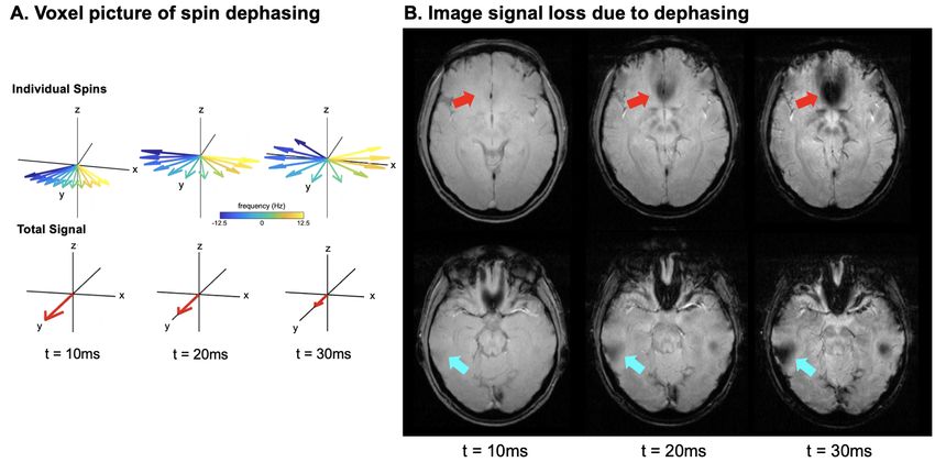
geometric distortions can still be present due to off-resonance errors in k-space encoding.
     It is also important to consider off-resonance artifacts and potential correction strategies when
working with MRI scanners that have more inhomogeneous B0 fields than high-field superconducting
magnets. Recently, there have been many advances in portable MRI at lower fields to perform in
vivo human imaging [18, 19, 20, 21, 22]. These new technologies are important for increasing
the accessibility of MRI [23], but they generally have less uniform B0 fields than superconducting
magnets and off-resonance correction approaches are needed. Low field MRI scanners built with
permanent magnets can also experience large field drifts due to temperature induced field changes,
so dynamic tracking of the B0 field strength is sometimes needed during imaging.
     This review is structured by first describing the sources of off-resonance in MR imaging in
Section 2 and their effects on imaging in Section 3. Section 4 details ways to estimate a B0
fieldmap using pulse sequence, hardware, and optimization based approaches. Section 5 discusses
strategies to prevent and correct for B0 artifacts, and Section 6 concludes the paper. All code for
the simulations shown here is available online at https://github.com/fmrilab/B0-review-2022,
including example code to perform model-based image reconstruction [24] that incorporates a B0
fieldmap [25] using the Michigan Image Reconstruction Toolbox (MIRT) [26].

2       Sources of magnetic field off-resonance
2.1     Main field inhomogeneity
2.1.1    Modern superconducting magnet homogeneity
The B0 polarizing fields of modern high-field superconducting magnets, most often at field strengths
of 1.5T or 3T, are generally very uniform, and after shimming with superconducting shim coils and
passive shim elements are on the order of 1ppm uniformity over a large imaging volume. Because of
this, artifacts from susceptibility, chemical shift, and metal implants (discussed in later sections) are
the dominant sources of B0 artifacts in high-field superconducting MRI scanners, and off-resonance
artifacts from the magnet itself are minimal.

2.1.2    New magnet designs for lower cost and portability
As more light-weight, low-cost, and portable MRI designs are being developed, permanent magnets
and resistive electromagnets are being chosen to create the polarizing fields. Both permanent
and resistive magnet designs are much less expensive to produce than superconducting magnets,
and, importantly, are much less expensive and easier to operate and maintain. However, these
magnets are generally less spatially homogeneous and may require B0 field correction even for
routine imaging. Permanent magnets have the advantage that they require no power or cooling
mechanism to operate, but they can be very sensitive to temperature induced field drifts, which
often need to be monitored during scanning. Resistive magnets are not as temperature sensitive,
but power consumption and cooling will need to be taken into consideration and will potentially

                                                   3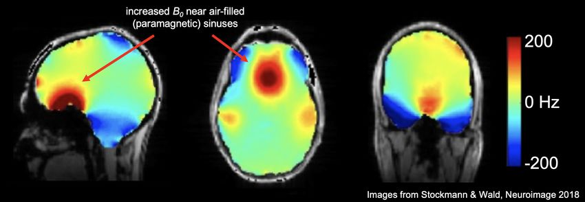
Direction of J Rel-         Relative Magnetic
 Magnetic Property          ative to External           Susceptibility (χ, in    Example Materials
                            Field                       ppm)
                                                                                 Water, most biological
 Diamagnetism               Opposite                    -10
                                                                                 tissues
 Paramagnetism              Same                        +1                       Molecular oxygen, O2
 Superparamagnetism         Same                        +5000                    SPIO contrast agents
 Ferromagnetism             Same                        >10,000                  Iron, steel

Figure 1: Magnetic Susceptibility. Adapted from https://mriquestions.com/what-is-susceptibility.
html [33]

limit the field strength and homogeneity.
     There are examples both in industry and academia of newer permanent magnetic designs. Cur-
rently available commercially scanners include a 64 mT portable brain scanner (https://www.
hyperfine.io), a 1T scanner for the neonatal intensive care unit (https://www.aspectimaging.
com), and a low-field system for dedicated prostate imaging and biopsy guidance (https://promaxo.
com). Academic groups have created permanent magnet designs using cylindrical Halbach geome-
tries [27, 28, 29], dipole magnet geometries [19, 18], and single sided designs [30]. Unlike supercon-
ducting magnets, these scanners have field homogeneities in the range of tens of ppm (for smaller
FOV extremity imaging) to hundreds or thousands of ppms for head imaging, but have been shown
to successfully image human subjects [20, 21, 19, 18].
     Resistive magnets at low field have also been explored. Obungoloch et al. designed and con-
structed a prepolarized MRI scanner that acquired phantom images at 2.66mT with a polarizing
field of 27mT, and a field homogeneity of 5000 ppm, similar to the level of inhomogeneity in the
permanent magnet Halbach designs [31].

2.2     Magnetic susceptibility
One of the largest sources of B0 inhomogeneity during routine in vivo MRI is magnetic susceptibility.
Magnetic susceptibility (sometimes called volume magnetic susceptibility) [32], denoted as χ, is the
property of a material to either strengthen (χ > 0) or weaken (χ < 0) an applied magnetic field,
based on its internal magnetic polarization, J, as follows:

                                                χ = J/B0                                               (1)

Magnetic susceptibility is unitless since it is the ratio of two fields, but it is often expressed in parts
per million (or ppm) for convenience in the context of MRI. For example, molecular oxygen, O2 ,
has a magnetic susceptibility of roughly +1ppm, which means that when in the presence of a 1.5T,
or 64 MHz, external magnetic field, its internal polarization will be roughly 1.5µT, or 64 Hz.
     If an object has non-uniform magnetic susceptibility, it will lead to a non-uniform magnetic
field, even within the most uniform of applied fields generated by today’s modern superconducting

                                                    4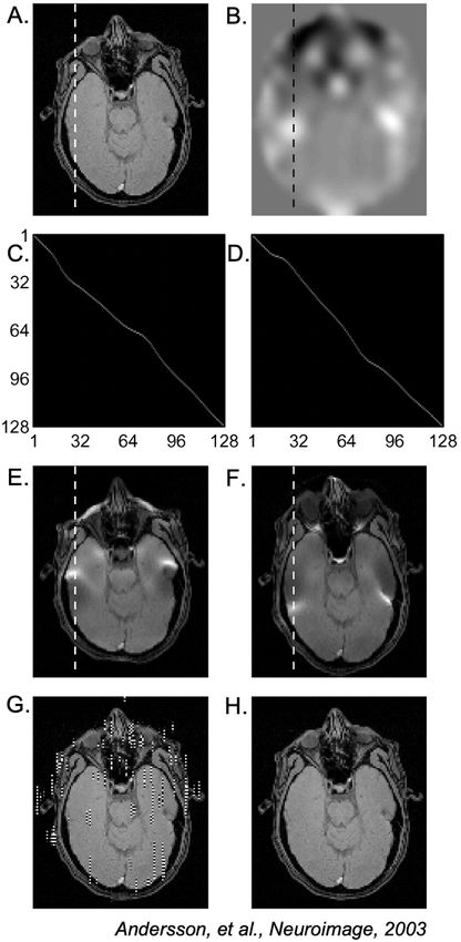
magnets. In human imaging, most biological tissues are weakly diamagnetic (χ < 0) and oppose the
applied field, but oxygen, present in the lungs, sinuses, and other air cavities, is weakly paramagnetic
(χ > 0) and strengthens the applied field. This leads to spatially varying B0 fields within the body,
such as the one shown in Fig. 2.
    Looking at Eq. (1), one can see that as the applied magnetic field B0 increases, the internal
polarization, J, will also increase. This means that at higher field strengths the amount of off-
resonance will increase, and therefore the susceptibility artifacts will be more severe [34].

Figure 2: B0 magnetic field in the brain at 7T with 2nd order shimming. This fieldmap shows the
spatially varying patterns of the B0 field in the human brain (superimposed over an anatomical image). Even after
2nd order shimming has been applied to flatten the field, higher order field inhomogeneities persist. Arrows show
that near the air-filled, and therefore paramagnetic, sinuses, the B0 field is higher than areas in the center of the
mostly diamagnetic brain tissue. (Images reused from Stockmann & Wald, 2018 [35] with permission.)

2.3     Chemical shift
Another source of off-resonance is the chemical shift in resonant frequency of different tissues in
the body. The most relevant source of chemical shift is from fat, which has a shift in frequency
of -3.5ppm relative to water [37]. At 1.5T (64 MHz), this corresponds to a shift in frequency of
64MHz × -3.5ppm = -224 Hz, and at 3T a shift of -448 Hz. The earliest accounts of chemical shift
image artifacts describe enhanced or diminished borders of organs within the body that have tissue
boundaries containing fat [38, 39]. This is due to the fat signal shifting within the image because
it is off-resonant compared to water (Eq. (7)). The directions and angles of the slice selection and
frequency encoding axes can also affect chemical shift artifacts, leading to them sometimes being
present and sometimes not, which can confound diagnosis and affect treatment [40]. Hood et al. [37]
provide a good review of how chemical shift artifacts impact clinical interpretation of images. The
authors also describe what are referred to as chemical shift artifacts of the 2nd kind, which are
not shifts in image space of the voxel, but rather a cancellation of the out-of-phase water and fat
components in the voxel that leads to a loss of total signal (see Hood et al. Fig. 10). These out-
of-phase images at a given TE can be compared to images with different TEs where fat is visible,
allowing the clear identification of fat.

                                                         5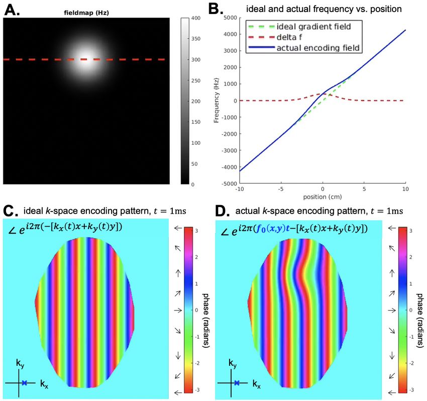
2.4    Metal implants
While magnetic susceptibility differences drive
many sources of B0 inhomogeneity as described
in Section 2.2, the B0 effects of metal implants
are different, mainly due to the sheer magnitude
of the B0 shifts, leading to effects that often re-
quire advanced measures to compensate. Most
metal implants in common use today are la-
beled as MRI-conditional, which indicates that
MRI scanning is acceptable provided the speci-
fied conditions for safe use are met [41, 42]. Al-
lowable or safe use, however, does not mean that
the quality of the images is not impacted by sus-
ceptibility effects around the implant.
     Hagreaves et al. [8] is a review on sources
and artifacts due to metal implants as well as Figure 3: Metal artifact from 50mT to 7T. Here
                                                      we show Figure 7 from Van Speybroek, et al., 2021 [36]
a compendium on the various approaches to where the “worst-case” scenario images for four types of
mitigate the artifacts. Jungmann et al. [43] metal implants are demonstrated. (Images reused via open
                                                      access license.)
also reviews mitigation methods and provides
numerous imaging examples.            As with all
susceptibility-induced B0 changes, these effects scale with field strength. Notably, lower magnetic
fields result in smaller distortions and lower field strength clinical scanners are often preferred when
scanning structures proximal to metal implants, as seen in Fig. 3. Further, the lower resonant
frequency at lower field reduces the safety and imaging impact of RF (B1 ) inhomogeneity around
metal implants.

3     Impact on Imaging
3.1    MRI Signal Equation Incorporating Off-Resonance
In an MRI experiment, the magnetic spins being imaged precess at resonant frequency ω:

                                                 ω = γB                                                 (2)

where γ is a spin’s gyromagnetic ratio and B is the magnetic field strength at the spin location.
For an 1 H proton in water for which γ/2π = 42.577 MHz/T, at a magnetic field strength B =
3T, the spins precess at roughly 128 MHz. Note that throughout this paper we may use “field” or
“frequency” depending on context, but the reader can convert from a precession frequency in Hz to
a magnetic field in T or vice versa by multiplying or dividing by γ/2π.

                                                     6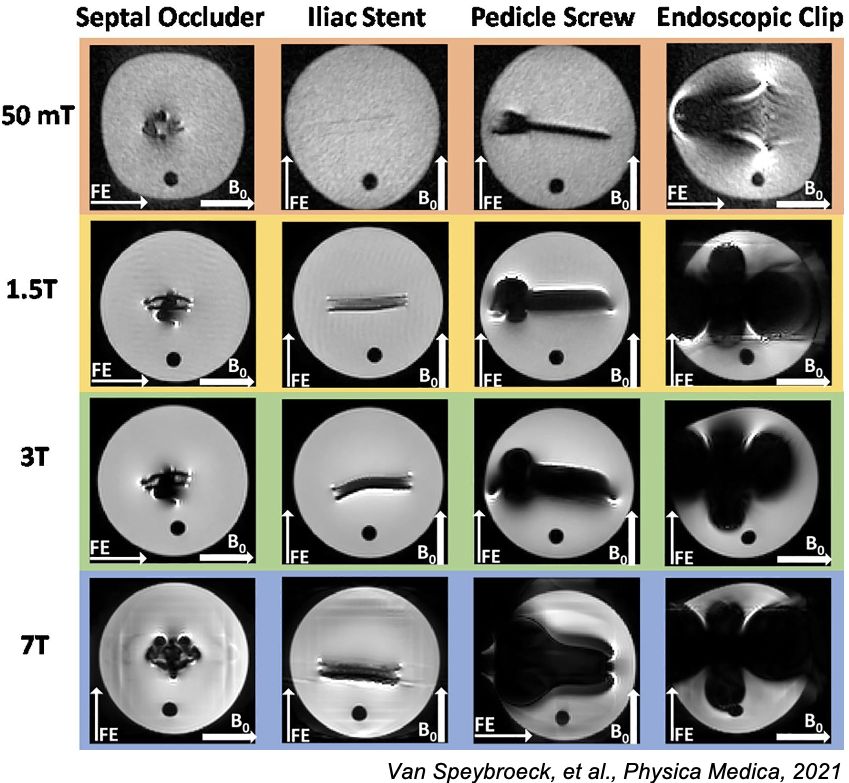
To create an image in an ideal MRI experiment, first, the object is placed in a spatially uniform
polarizing field, B0 . The 1 H spins throughout the entire object will now be precessing at ω0 .
Next, spatially varying magnetic fields, Gx , Gy , and Gz , referred to as “gradient fields” or simply
“gradients”, are applied to linearly change the magnetic field as a function of spatial position,
which therefore changes the precession frequency of spins at different locations, i.e., ω(x, y, z) =
γ(B0 +Gx x+Gy y +Gz z). By applying different gradient fields over time, spins at different locations
can be encoded, the most common method being Fourier space, or k-space, encoding. The MRI
signal as a function of these time-varying gradients can be described using the signal equation:
                         Z                                                             Z    τ
                                          −i2π[kx (t)x+ky (t)y]                    γ
                s(t) =       m(x, y)e                             dxdy , kα (t) =               Gα (τ )dτ   (3)
                                                                                  2π    0

where s(t) is the time-varying MRI signal, m(x, y) is the magnetization at location (x, y), and kx (t)
and ky (t) are the k-space sampling locations. For brevity, the equation above and the rest of the
image encoding mathematics will be in 2D, but it can be extended to 3D as well by adding a third
z term to the exponent in Eq. (3).
    By having a uniform polarizing B0 field, the time-varying signal s(t) is only a function of the
applied gradients. When B0 is not spatially uniform, we must add a term to the signal equation for
the additional spatially dependent phase, φ(x, y), accrued over time t:

                             φ(x, y, t) = γB0 (x, y)t = ω0 (x, y)t = 2πf0 (x, y)t                           (4)

    The phase can now be added to the signal equation using a complex exponential of the product
of the fieldmap and the time, t:
                                      Z
                             s(t) =        m(x, y)e−iω0 (x,y)t e−i2π[kx (t)x+ky (t)y] dxdy                  (5)

This leads to a breakdown of the encoding properties of the MRI signal equation, since now there
will be additional phase in the object that is not a result of the k-space encoding. Depending on the
length of the readout, the type of k-space acquisition, and other scan parameters, the excess phase
accrued due to off-resonance can lead to various types of artifacts such as signal loss, distortions,
and blurring.
Signal Loss
When spins in a voxel have different resonant frequencies due to rapid spatial variations in the B0
field, spins will dephase as seen in Fig. 4 (images in Fig. 4 were acquired from a healthy subject
after obtaining IRB approved written informed consent). Immediately after RF excitation the
spins are all aligned, but during the course of the readout the spins dephase and there is destructive
interference in the voxel, referred to as T2∗ decay. The most common way to deal with this signal
loss is through the use of spin echoes [11]. In a spin echo sequence, the spins are flipped into
the transverse plane, and then after time TE/2, a 180◦ RF pulse flips the spins about one of the

                                                              7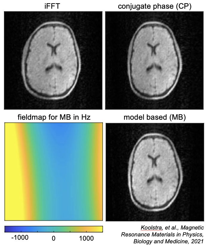
Figure 4: Signal Loss from Spin Dephasing.                  A. Voxel view of spin dephasing. Spins with different
off-resonance will gain different amounts of phase during signal readout leading them to “fan out”, and eventually
completely cancel each other. B. A gradient echo image is shown for two different slices at three different echo times
(TE). At the later echo times, signal loss due to dephasing is present as indicated by the arrows.

transverse axes. Then, after precessing for time TE/2, the spins will refocus at the echo time, TE.
Spin echoes are very robust overall, and because of this spin echo based sequences have been the
pulse sequence of choice for many of the academic low field scanners [20, 21, 19, 31], as well as the
commercially available 64 mT portable brain scanner [22].
Image Encoding Artifacts: Distortions & Blurring
Spin echoes can mitigate much of the off-resonance based signal loss, but even using spin echo
sequences, significant off-resonance artifacts can be present based on image encoding errors, such
as distortion [44], blurring, and pile-up. Looking at Eq. (5), the reduction of intravoxel dephasing
by using a spin echo leads to an apparent increase in the m(x, y) term, but the spatial encoding in
the exponential of that equation will still be affected by B0 effects. When there is a non uniform
fieldmap like the one in Fig. 2, there is a breakdown in the encoding since it is not only scanner
gradient k-space encoding that is contributing to a voxel’s phase, but also phase accrued due to
off-resonance. We can factor out 2π and combine the exponentials into one term as follows:
                                        Z
                               s(t) =       m(x, y)e−i2π[f0 (x,y)t+[kx (t)x+ky (t)y]] dxdy                        (6)

If [kx (t)x + ky (t)y] >> f0 (x, y)t, s(t) will accurately encode the object at m(x, y) for k-space
location (kx (t), ky (t)). However, if there is large off-resonance (or long time t), the phase pattern
associated with the encoding will be warped, as seen in Fig. 5. In Fig. 5, the ideal vs. the actual
encoding pattern, i.e., the phase of the complex exponential in Eq. (6), to acquire the sample at

                                                            8
(kx , ky ) = (0, 0.426 cm−1 ) is shown, assuming t = 1ms and a perfect rectangular gradient pulse of 1
mT/m was played (in practice much larger gradients are used in an MRI experiment, but to allow
visualization a smaller gradient is simulated here). As described in more detail below, for Cartesian
sequences this encoding error normally manifests in geometric distortions, and for non- Cartesian
sequences, such as spiral, this will result in both distortions and blurring.
3.2 Utility of long readouts
In an examination of Eq. (4), we can see that off-
resonance phase accrual is linearly dependent
on the time since excitation. This can be split
into two parts: the phase accumulation to the
echo time (TE) and phase accumulation during
k-space scanning. The first term contributes
to signal loss in the m(x, y) term in gradient
echo imaging. The second term contributes to
k-space distortions and is effects, as shown in
Fig. 5. Thus, long readouts for imaging will
show increased distortions. That said, there are
advantages to having longer readouts in terms
of SNR, k-space scanning efficiency, and overall
acquisition speed.
Figure 5: Ideal vs. actual k-space encoding. A.
3.2.1 SNR
Simulated off-resonance fieldmap in Hz. B. 1D plots of the
For a given repetition time (TR), flip angle, encoding fields as a function of position, where the red dot-
ted line correspond to the dotted red line in A. C. The ideal
and spatial resolution, the signal to noise ratio k-space encoding phase for (k , k ) = (0, 0.426 cm−1 ). D.
x y
(SNR) is proportional to the square root of the The actual k-space encoding phase. When performing a
2D iFFT for image reconstruction, the data is assumed to
total acquisition time, TA/D [45], at least to a be acquired with encoding as shown in C, but with off-
first approximation. The total acquisition time resonance the encoding pattern will be that shown in D,
leading to geometric distortions.
here is defined the sum of the length of all ac-
quisitions contributing to a given image. One
can also define SNR efficiency as the SNR divided by the square root of overall time to acquire
an image. Thus, as one increases the time spent acquiring data in each TR, SNR efficiency also
increases.
3.2.2 k-space scanning
Long readouts following each RF excitation enable rapid k-space scanning and hence reduced total
scan times. In general, reduced study duration is beneficial for patient comfort and for economic
reasons. Beyond that, accelerated imaging is also enabling for many applications. While there
are numerous methods to accelerate imaging, notably parallel imaging, k-space scanning with long
9readouts also plays an important role in reducing scan time. For example, in dynamic imaging
applications like cardiac imaging, there may be advantages to acquiring a larger part of k-space
with each excitation so that higher resolution images can be acquired during a breath hold. In
neuroimaging, the ability to “freeze” motion has led to single shot k-space scanning to be the
dominant methods for acquiring diffusion weighted and BOLD functional brain images. These are
but a few examples where long readout and k-space scanning are useful in MRI.
3.3 Cartesian imaging: spin-warp and EPI
In Cartesian imaging, data is sampled along straight line segments along kx . The term “Cartesian”
implies that the samples are regularly spaced, though in practice the kx dimension is sometimes
sampled along the trapezoidal gradient ramps (in addition to the plateau) for increased scan effi-
ciency. Since the invention of MRI, Cartesian imaging has remained the “bread and butter” MRI
technique despite its relatively low scan-time efficiency compared to non-Cartesian imaging, since
(i) it allows fast and simple reconstruction using inverse Fast Fourier Transforms (iFFT), (ii) image
artifacts due to off-resonance and chemical shift are often easy to recognize and “read through”,
and (iii) geometric distortions can be corrected using fast and widely available methods.
3.3.1 Spin-warp imaging
To understand the impact of off-resonance and chemical shift on Cartesian imaging, consider first
the case of “spin-warp” imaging, where a single line along kx is sampled after each RF excitation,
with constant gradient amplitude Gx . In this case the kx -encoding term in Eq. (6) can be written
γ
as kx (t) = 2π Gx t and (since the acquisition bandwidth along ky is effectively infinite) the exponent
in Eq. (6) becomes −i2πkx [x + δx] − i2πky (t)y where
2πf0 (x, y)
δx = . (7)
γGx
In other words, a voxel at position x with off-resonance frequency f0 will appear at x + δx in
the reconstructed image. For typical readout bandwidths, δx is negligible for most tissue types at
clinical field strengths, but can be on the order of a voxel width, e.g., fat. As a consequence, the
acquisition bandwidth for most clinical sequences is kept sufficiently high to avoid significant fat
shift. Note that Eq. (7) ignores any B0 inhomogeneity within the voxel centered at location (x, y),
and hence does not describe any signal loss that may occur at a given echo time (TE).
3.3.2 Echo-planar imaging
In echo-planar imaging (EPI), multiple lines at different ky -encoding levels are acquired after each
RF excitation. This is done by playing a small y-gradient trapezoid “blip” after the end of each
kx line, and then traversing the subsequent line in reverse direction (non-flyback EPI). Assuming
regular sampling along ky with subsequent “echoes” spaced τs apart in time, and ignoring the
(typically small) shift δx along the frequency-encoding direction, the exponent in Eq. (6) becomes
10−i2πkx x − i2πky [y + δy] where
2πf0 (x, y)
δy = (8)
γGy
is the spatial shift (along y) in the reconstructed image. Here, Gy is the average gradient amplitude
of the y blip over the echo time spacing τs , which is much smaller than the readout gradient
amplitude Gx in Eq. (7). As a result, EPI can produce substantial spatial shifts along ky .
3.3.3 Interleaved and readout mosaic segmented EPI
EPI comes in several multi-shot variants that make various tradeoffs between image artifacts and
scan efficiency. In addition to geometric distortions as just described, another consideration is T2∗
decay during the echo train, which acts as a k-space filter resulting in blurring in image space.
In interleaved EPI, the area of each ky -encoding blip, and hence Gy , is increased, making each
EPI train undersampled by a factor equal to the number of segments (shots) Ns . This reduces
the geometric shifts, and the time allowing for T2∗ decay, by that same factor Ns . Interleaved EPI
is typically implemented by shifting the start of subsequent EPI segments by a time n/τs where
n = 0, ..., Ns − 1 is the shot number, to avoid abrupt phase jumps in ky -space due to off-resonance.
A potential drawback of interleaved EPI is shot-to-shot variability in the acquired data, resulting
from, e.g., physiological fluctuations or subject motion.
An alternative scheme useful for diffusion MRI is readout mosaic segmented EPI, where only a
portion (“blind”) of kx -space is acquired during each shot, while sampling all desired ky locations
per shot [46, 47]. The advantage of this approach is that it preserves the regular sampling along ky
in the presence of shot-to-shot k-space shifts due to rotational motion in the presence of diffusion-
encoding gradients [48]. By introducing a small overlap between blinds along kx , such shifts need
not introduce any gaps along kx as well. A drawback of this approach is that the echo time spacing
is not reduced by the full segmentation factor Ns due to finite gradient rise time, and hence the
reduction in geometric shift is somewhat smaller than for interleaved EPI for a given Ns .
3.4 Non-Cartesian acquisitions
While much of MRI carried out on clinical scanners uses Cartesian acquisitions like spin-warp or
EPI, there are numerous useful applications that use non-Cartesian acquisitions. This is a broad
class of image acquisitions that typically do not acquire data along parallel lines in k-space. Some
aspects are similar to Cartesian imaging, for example, the need to acquire data over a prescribed
area in k-space for the desired spatial resolution and to acquire k-space data with sufficient sample
density to prevent aliasing. The nature of the off-resonance artifacts, however, are quite different.
Below, we discuss these effects for radial line and spiral imaging, but note that there are yet other
non-Cartesian trajectories, e.g., rosettes [49], that have quite complicated off-resonance behavior
that is beyond the scope of this review.
113.4.1 Radial line and spiral imaging
Radial line and spiral imaging are useful in a number of applications. For example, radial line
acquisitions in 2D or 3D have substantial utility in zero- and ultra-short TE (ZTE and UTE)
imaging [50, 51], angiography [52], and contrast enhanced abdominal imaging [53]. Spiral imaging
has been shown to be useful in functional MRI [54], cardiac imaging [55], and brain imaging [56].
Spiral and radial line imaging have off-resonance features that are similar to each other, but are
quite different from spin-warp and EPI. For each line of a radial line acquisition, there is a shift in
the radial direction in the form:
2πf0 (x, y)
δr ≡ (9)
γGr
where Gr is the strength of the radial gradient. Since the direction of the radial gradient is constantly
changing and ultimately points in all directions, the net effect is not a single shift, but a shift in
all directions. More specifically, any off-resonant point in the object maps to a ring-like response
of radius δr. This is equivalent to saying that the point spread function (PSF) or impulse response
is this ring-like function, the radius of which, δr is proportional to the off-resonance frequency,
f0 (x, y). For a complex image, this manifests as a blur of radius δr.
For spirals, the off-resonance response is again a radial shift in all directions, with amplitude:
2πf0 (x, y)
δrs ≈ (10)
γGr
where Gr is the average outward component of the spiral gradients. One can also infer the average
outward component with Gr = 2πkmax /T , where T is the length of the spiral readout. Now, any
off-resonant point in the object maps to a ring-like response of radius δrs and as with radial imaging,
this is proportional to the off-resonance frequency, f0 (x, y). As can be seen from the alternate Gr
expression, the blur is also proportional to length of the spiral readout, T . Again, for a complex
image, this manifests as a blur of radius δrs . For spiral imaging, the relationship that the blur is
a ring of radius δrs is only approximate because the average outward component typically varies
during the readout making the actual blur function a bit more complicated. Still, the main principle
is that longer readouts make the off-resonance image blurring worse.
The off-resonance behavior also extends to three dimensions. For examples, ZTE imaging and
angiography applications often use a 3D radial line acquisition. While spirals don’t extend directly
to 3D, there are 3D trajectories like 3D cones, yarnballs, and spiral-radial hybrids [57] that have
off-resonance properties similar to spirals. In these cases, we consider induced blur to be occurring
in all three dimensions, that is, the PSF or impulse response is an annular sphere with radius δr (or
δrs ). Again, greater off-resonance and longer readouts increase the radius of the blurring function.
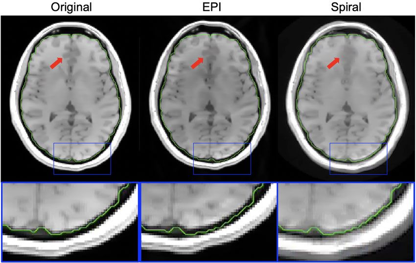
The ways that off-resonance affects EPI and spiral images at 3T is shown in Fig. 6 (images
in Fig. 6 were acquired from a healthy subject after obtaining IRB approved written informed
consent). As expected the artifacts in the spiral image are primarily blurring, and the artifacts
12Figure 6: Image simulations: Cartesian vs. non-Cartesian. Here we show the different off-resonance
effects from EPI vs. spiral acquisition. In the EPI image, geometric distortion of the brain is visible, including the
zoomed-in region in the visual cortex, where the brain has been compressed compared to the original. In the spiral
image, there is a large amount of blurring in the frontal cortex due to its location closely superior to the sinuses,
noted by the red arrow, but there is less geometric distortion than in EPI.
in the simulated EPI image are primarily geometric distortions along the phase encode (vertical)
direction. Additional details on the simulation can be found at https://github.com/fmrilab/
B0-review-2022.
3.5 Imaging near metal implants
Though not ferromagnetic, the susceptibility differences between metals and tissues are substantially
larger than the differences between tissues and the surrounding air. These large susceptibility dif-
ferences, in combination with the often large mass of these implants, lead to similar, but magnified,
B0 effects. For example, much of GRE imaging is infeasible in close proximity to implants, except
for the very shortest TEs, meaning that most studies use SE or Fast/Turbo Spin Echo (FSE/TSE)
acquisitions. Similarly, rapid imaging methods like EPI or spiral imaging with implants will typi-
cally produce artifacts that are too severe to correct. There are often severe geometric distortions
in the readout (frequency encoding) direction associated with implants, including signal voids and
piling up artifacts. Another common issue is the distortion of the slice profiles, where there can be
spatial displacement several slice thicknesses in magnitude, distorted slice profiles like potato chips,
and variable slice thicknesses. In both frequency encode and slice effects, the spatial distortions are
13proportional to the frequency offset divided by the bandwidth per pixel (or slice thickness).
4 Estimating B 0 Field Inhomogeneity
4.1 MRI sequences for acquiring fieldmaps
Before correction for B0 inhomogeneity artifacts, it is often necessary to acquire and estimate the
fieldmap. The simplest way to estimate a B0 fieldmap is to create a pulse sequence that acquires two
sequential gradient echo images at different TEs, and then subtract their relative phases to obtain
the amount of precession at that voxel over the echo time difference ∆TE. The phase difference is
then scaled by ∆TE to get the fieldmap:
∆φ(x, y) = ∠m(x, y, TE1 ) − ∠m(x, y, TE2 ) (11)
∆φ(x, y)
∆ω0 (x, y) = (12)
∆TE
This is the basic idea behind B0 fieldmapping in MRI, but there are many ways to estimate a
fieldmap within this general approach. The choice of ∆TE will affect the quality of the fieldmaps,
and has been quantitatively evaluated in prior work [58]. Normally gradient echo images at short
TEs are used to avoid distortions in the underlying fieldmap, but for applications using EPI, there
has also been work in using EPI-based fieldmaps [59]. While EPI fieldmaps will be distorted given
the longer TEs required, they have the advantage that they will be distorted in the same way and
also experience the same eddy currents as the EPI data used in the imaging experiment, potentially
allowing for easier look up of the off-resonance at any voxel.
Another consideration when calculating fieldmaps is phase wrap. A longer ∆TE is desirable
because it will increase the SNR of the phase difference measurement. However, when ∆TE is
increased, more phase wrap can occur. Fortunately, many tools such as FSL [60] include phase
unwrapping algorithms that are useful when calculating off-resonance field maps, such as the auto-
mated method introduced by Jenkinson in 2003 [61].
There have also been recent approaches to rapidly acquire B0 fieldmaps along with transmit
coil patterns (B1+ ), receive coil sensitivity (B1− ), and eddy current maps in as little as 11s at
1×2×2mm3 resolution at 3T [62]. This kind of approach is especially useful for model-based image
reconstructions that incorporate B0 (see Section 5.4), since B1− maps are often needed as well.
4.2 Hardware methods
In addition to measuring a fieldmap using a sequence, it is possible to employ external hardware
and/or built in scanner hardware to monitor changes in off-resonance. Generally these types of
hardware tracking methods will be used for dynamic B0 correction (see Section 5.5) after an ini-
tial B0 map has been measured using a fieldmapping sequence. One option is to use NMR field
probes [63, 64, 65], which measure the changes in phase of the MRI signal within small external
14samples. These probes are now commercially available (https://skope.swiss/) and have been
used in applications such as diffusion MRI, fMRI, and ultra high field imaging. Another approach is
to use FID measurements from a multicoil receive array, which can encode changes in signal based
on the different spatial locations of the coils. By combining with a reference image from each coil,
Wallace et al. showed that FIDs can be used to dynamically track up to 2nd order field changes [66].
4.3 Optimization and smoothing methods
After multi-TE data has been acquired, Eq. (12) is the simplest way to calculate a fieldmap, but
the maps are often improved by using some form of smoothing or regularization due to the difficulty
of getting B0 values near the edges of anatomy. In the original TOPUP paper [67], a smoothed
version of the fieldmap that is based on polynomial fitting was used. The work by Hutton et al. [58],
in addition to examining ∆TE, also quantitatively evaluates how the amount of smoothing used
affects fieldmap estimates.
There are also optimization-based approaches that use a multi-term objective function, where
the phase differences between multiple TEs is a data fit term and another regularization term
penalizes rapidly varying and sudden field changes [68]. This method has been expanded upon
to incorporate a more efficient optimization algorithm and the ability to input multicoil data [69].
Additionally, it is possible to jointly optimize for a fieldmap and an image, and these approaches
are described in Section 5.4 on model based image reconstruction.
5 Correction Strategies
In this section we discuss strategies to correct for off-resonance artifacts in MRI. Many of the
methods described could fit into multiple categories, but we have broadly categorized them to help
in describing the different options available to MRI users, as outlined in Figure 7.
Artifact Prevention (Section 5.1) B0 Correction Methods (Sections 5.2-5.6)
• EPI/Cartesian focused
• Hardware based
– Image Space: TOPUP
– passive & active shimming
– PSF
– lower-field MRI
• Non-Cartesian focused
• Sequence based
– Direct/Analytical: conjugate phase, SPHERE
– spin echoes
– Autofocusing
– shorter readouts: parallel imag-
• Model based image reconstruction including B0
ing, multishot imaging
• Dynamic corrections
– fat suppression / nulling (STIR)
• Corrections for larger B0 shifts around metal implants
– smaller voxels: parallel imag-
– View angle tilting
ing, simultaneous multislice
– MAVRIC
– SEMAC
Figure 7: Common B0 artifact mitigation strategies.
155.1 Artifact Prevention & Reduction
5.1.1 Hardware based artifact mitigation
The most straightforward way to prevent B0 artifacts is to have as uniform a field as possible
before starting a scan, and the process of refining the uniformity of the B0 field is referred to as
shimming [70]. Shimming can be done either by improving the static B0 field hardware (i.e., with
superconducting shim magnets or ferrous passive elements) or by actively changing the currents in
the scanner’s electro-shim coils, which include the gradient coils. An example of passive shimming
at low field is the work of Liu, et al., where on their 50mT scanner they originally had a 2000
ppm peak-to-peak uniformity over a 24cm diameter spherical volume (DSV) within their SmCo
dipole magnet, but after adding smaller passive shim magnets their uniformity was increased to 250
ppm [19]. Automated shimming is a standard part of a clinical MRI pre-scan calibration (at least
for the constant linear shims terms) and for most users this will be automatic, but for certain types
of acquisitions, such as MR spectroscopy that requires a very uniform field [71], the user may need
to do manual shimming as well.
In addition to shimming, using a lower magnetic field is a direct way to reduce B0 artifacts. As
was discussed in Section 2, B0 field changes from susceptibility and chemical shift scale with field
strength, so these artifacts are generally worse at higher field. There are some B0 artifact mitigation
strategies that are harder at low field due to decreased SNR, but in general going to lower field will
reduce signal loss and encoding artifacts from an inhomogeneous field.
5.1.2 Sequence based artifact mitigation
When designing an MRI sequence, parameters can be adjusted to reduced the effects of off-
resonance. Using a short readout time (high acquisition bandwidth) will limit the amount of
extra phase accrued due to off-resonance and therefore reduce artifacts. The use of parallel imaging
techniques [13, 72] is an effective way to reduce the readout length of a scan, by allowing the user
to collect less k-space data each shot. If using longer readouts, spin echoes and spin echo trains
will refocus spins and avoid much of the T2∗ signal loss [11, 12]. Chemical shift artifacts can be
avoided by using a short time inversion recovery (STIR) sequence that nulls recovering fat signal,
inserting fat saturation modules before water excitation (an RF excitation at the fat frequency and
then a large crusher gradient), or by using a spectrally selective RF pulse centered around the water
resonant frequency [73]. Further, while this generally has the downside of longer scan time due to
additional encoding, using smaller voxels will decrease the possible signal loss due to a more local
neighborhood of spins being averaged in each voxel. Parallel imaging and simultaneous multislice
imaging [14] are effective strategies to reduce voxel size without increasing scan time.
5.2 EPI
Several methods for correcting geometric and intensity distortions in EPI have been proposed (see,
e.g., [75, 76] for recent overviews), and here we focus on three of the more popular ones: image-
based correction using an acquired B0 map, image-based correction using two reference scans with
16opposite phase-encode blip directions, and the point-spread function (PSF) mapping approach.
These have all proven to be useful for EPI distortion correction in fMRI and diffusion imaging.
5.2.1 Fieldmap based correction
One popular approach is based on the separate acqui-
sition of an undistorted B0 map (e.g., using spin-warp
3D GRE), that is used to calculate the shift δy (Eq. (8))
for each spatial location [67]. The pixel values in the
reconstructed (distorted) image are then shifted along
the phase-encode direction by −δy. This is followed by
an intensity correction step based on the spatial gra-
dient of δy [67]. Potential drawbacks of this approach
include inaccurate correction near object edges due to
inaccurate B0 estimates (partial-volume effects), and
inability to resolve overlapping pixels.
5.2.2 Opposite phase-encoding scans
Another widely used approach that also operates on
magnitude images is TOPUP [74], that uses as input
two EPI images that differ only in the sign of the phase-
encoding blips (i.e., traversing ky in the positive and
negative, or bottom-up and top-down, directions). The
TOPUP model is
" # " #
f +,i K +,i
= xi (13)
f −,i K −,i
where xi is the ith column (along y) of the undistorted
true image x, f + and f − are the distorted bottom-up
and top-down images, respectively, and K +,i and K −,i
are real-valued square matrices that map the pixel lo-
cations in the true image column xi to the observed Figure 8: Illustration of EPI distortion
correction using Eq. (13). (A) Ground-truth
image columns f +/−,i . In the absence of B0 inhomo- (undistorted) object and (B) fieldmap. (C,D)
geneity, K +,i and K −,i would be the identity matrix K +,i and K −,i for the dashed lines in (E,F). (E,F)
Distorted images f + and f − . (G) Distortion cor-
I. rection attempt using only f + . (H) Successful dis-
With knowledge of B0 (which determines K +,i and tortion correction using Eq. (13). (Images reused
from Andersson et al., 2003 [74] with permission.)
K −,i ), Eq. (13) can be inverted to obtain a least-
squares estimate x̂ of the true image, with the benefit
that pixels that overlap in one of the images (causing either K +,i or K −,i to be singular) are sep-
arated in the other, which enables the underlying true image to be resolved. In the absence of B0
17inhomogeneity, x̂i is simply the average of f +,i and f −,i . Furthermore, the TOPUP model can be
used to estimate B0 from the two EPI scans (obviating the need for a separately acquired B0 map),
by enforcing consistency between the observed images f +,− and the predicted images fˆ+,− created
by distorting x̂ using Eq. (13):
" # " #
2
f+,i K+,i (bi )
bˆi = arg min − x̂i (bi ) (14)
bi f−,i K−,i (bi ) 2
where bi parametrizes the displacements (using the notation from [74]), and we have made the
dependence of x̂i on bi explicit. Knowledge of bi yields an estimate of the field map B0 , which can
then be used to create an undistorted image using the approach described above. Advantages of this
approach include estimation of δy (Eq. (8)) from fast EPI scans, and avoiding potential inaccuracy
issues in the directly acquired B0 maps.
5.2.3 Point-spread function mapping
Another way to obtain δy(r) is based on measuring the point-spread function (PSF) along y [77,
78, 79]. This can be done by performing a calibration prescan wherein one adds an additional ky
encoding blip prior to the EPI readout, and repeats the measurement with different blip areas. For
a 2D EPI acquistion, this additional “constant-time” encoding yields a 3D dataset where the spatial
profile in the constant-time encoding dimension is the PSF [77]. The pixel shift can then be obtained
as the center (peak) of the PSF [79]. An advantage of this approach is that the shift is estimated
with the same EPI readout as the imaging sequence to be corrected, and hence experiences and
accounts for the same eddy currents and concomitant gradients.
5.3 Non-Cartesian
Off-resonance effects lead to burring and other distortions for non-Cartesian acquisitions, and this
is often more objectionable than the geometric distortions seen in Cartesian imaging. Thus, it is
often necessary to do some sort of off-resonance correction in order to produce clinically useful
images. This section describes common approaches for this correction that are applicable to radial
line, spiral, and related k-space trajectories.
5.3.1 Direct/Analytical Methods
Conjugate phase (CP) reconstruction In the absence of off-resonance, the signal equation in
Eq. (6) can be seen as a simple Fourier transform and a good image reconstruction will be simply
an inverse FFT. For a non-Cartesian acquisition, one can implement an approximate iFFT as:
1 X
m̂(x, y) = wi yi ei2π(kx,i x+ky,i y) ≈ F −1 {y(t)} (15)
M i
where i is the index over M k-space samples yi = y(ti ) at k-space locations (kx,i , ky,i ), and wi is
the sample density compensation term that accounts for uneven distribution of k-space samples
18common in non-Cartesian methods. In practice, this expression is commonly implemented by some
sort of interpolation in the k-domain to a Cartesian grid (known as gridding) followed by iFFT
operators or by using integrated functions like the NUFFT [80].
When considering off-resonance effects, a good image reconstruction may be to compensate for
the off-resonance phase accumulation in the image reconstruction at every time point and for each
location (x, y) [81, 82] as shown here:
1 X
m̂(x, y) = wi yi ei2π(f0 (x,y)ti +kx,i x+ky,i y) (16)
N i
where the f0 (x, y)ti term is known as the conjugate phase (CP) correction for the off-resonance (see
Fig. 9 for an image example).
There are limitations to the CP reconstruction, notably in that it is not a true inverse, but rather,
an approximation. In particular, this approach fails to make high quality image reconstructions
when the magnetic field (f0 (x, y)) varies rapidly in space and therefore the ring-like PSF will also
vary rapidly in space. If two PSFs overlap in space and these PSF functions are different, then this
approach cannot fully correct for both blurring functions. An alternate way to think about this is
that rapidly varying f0 corresponds to a local gradient, and therefore, the k-space is distorted for
locations with large local gradients [83]. The distorted local k-space limits the effectiveness of the
CP reconstruction. Model-based image reconstruction, described below, is more robust to address
rapid variations in the field map.
Efficient approximations While Eq. (15) has fast implementations with gridding or the NUFFT,
Eq. (16) is no longer an inverse Fourier transform due to the f0 (x, y)t term. Still, there are com-
putationally efficient implementations that result from decomposing this term into a sum of terms
that vary only in space and terms that vary only in time. The exponential can be modeled as a
summation of basis functions [85, 86]:
L
X
i2πf0 (x,y)t
e ≈ bl (t)cl (x, y) (17)
l=1
where bl and cl represent the basis functions for the time and image space, respectively. Note that
frequency, f0 (x, y), varies only with space.
The first such implementation was the so-called time-segmented approximation [87] to the CP
correction term, where bl = bl (t − t̄l ) is a family of time-varying weighting functions centered at t̄l
and cl = ei2πf0 (x,y) t̄l is a spatially varying phase function corresponding to t̄l . This approximation
to Eq. (16) is:
XL
m̂(x, y) ≈ F −1 {bl (t − t̄l ) y(t)}ei2πf0 (x,y) t̄l (18)
l=1
where F −1 is the gridding or NUFFT inverse transform of windowed segments of y(t). A related
19form is known as the multifrequency interpolation (MFI) method [88, 89], which modulates the
acquired data at frequencies fl using bl = ei2πfl t and interpolates between modulated images using
cl (x, y). This approximation to the CP reconstruction is:
L
X
m̂(x, y) ≈ F −1 {e−i2πfl t y(t)} cl (f0 (x, y) − fl ). (19)
l=1
Observe that L Fourier transforms are implemented in both of these approximations, so while they
are about L times slower than Eq. (15), they are still substantially faster than the discrete Fourier
transform implementation of Eq. (16).
Both the time-segmented approximation
and the MFI methods perform similarly and
can be viewed as low-rank approximations to
the ei2πf0 (x,y)t term. The interpolation functions
can be selected optimally according to different
optimality criteria [89, 85].
Deblurring with deconvolution While the
above approaches implement off-resonance cor-
rection as part of the image reconstruction, this
can also be implemented in the image domain
using deconvolution [90]. Provided the spatial
extent of the PSF or blurring function is small,
one can deblur the images using a space variant
deconvolution, where the deconvolution kernel
is guided by the acquired fieldmap. In Ahunbay
et al. [90], it was shown that in some circum-
stances the deconvolution kernel is separable in
x and y, which can greatly reduce the compu- Figure 9: CP and MB reconstruction at 50mT.
tational burden. Compared to a standard iFFT reconstruction, CP and MB
reconstructions both correct for geometric distortions due
Simulated phase evolution rewinding to off-resonance, especially in the right side of the brain
where the magnetic field off-resonance is stronger. MB
(SPHERE) An alternate approach to field also shows more uniform signal intensity. (Images reused
correction that is similar to the CP approach from Koolstra, et al., 2021 [84] via open access license.)
is to apply the CP correction to the forward
Fourier transform rather than the inverse trans-
form. This general approach is known as simulated phase evolution rewinding (SPHERE) [91]. The
approach starts with a reconstruction (iFFT) that does not apply an off-resonance phase correction,
e.g., Eq. (15), and follows it with a forward transform back to the k-domain, however, during the
20forward Fourier transform, the conjugate phase correction is applied:
X
ycorr (t) = m̂(x, y) e−i2π(f0 (x,y)t+[kx (t)x+ky (t)y]) (20)
x,y
where the sign of the complex exponent −f0 (x, y) is opposite of that in the signal equation Eq. (6),
thus applying the conjugate phase to compensate for the off-resonance phase accumulation. This
is followed by a simple iFFT to produce the final image. As with the CP reconstruction, the
f0 (x, y)t term means the forward transform is no longer a Fourier transform, but the time segmented
approximations and the MFI can be used to implement this in a computationally efficient manner.
Schomberg’s review [92] provides a detailed mathematical analysis of CP and SPHERE methods,
along with fast implementation strategies and timing comparisons of the different approaches.
5.3.2 Autofocusing
One unique aspect of non-Cartesian imaging is that the PSF may allow for autodetection of off-
resonance based on features of the image. Conceptually, it is like an autofocus camera where
different parts of the image have different off-resonance corrections to produce a fully deblurred
image. This is done by examining image features rather than through the use of a fieldmap. In [93],
a multi-frequency reconstruction was used, in which non-Cartesian images were reconstructed to
produce a family of images where different parts of each image are unblurred. An image metric
based on a measure of how closely the phase of low spatial frequency images aligned with the phase
of high spatial frequencies was used to determine, for each voxel (x, y), which modulated image
was sharpest. This measure works well for spiral imaging because the low spatial frequencies are
acquired earlier than high spatial frequencies, and off-resonance will lead to these components being
out of phase. In recent work [94], real time speech MRI with spiral readouts were automatically
deblurred using a sharpness metric of features in the vocal tract. Interestingly, these autofocus
methods can produce a fieldmap based on the selected image.
Machine Learning One challenge to autofocusing is the selection of an appropriate measure of
image sharpness. Because of the predictable and reproducible nature of the off-resonance effects in
non-Cartesian imaging, it is possible to train a neural network to learn and remove image blurs.
In [95], body imaging with 3D cones trajectories and long readouts were deblurred by a convolution
neural network (CNN) that directly maps blurred images to unblurred images acquired with shorter
readouts (but an overall longer scan time). This type of approach has also been applied to speech
MRI, where a longer readout image was deblurred using a CNN, allowing for longer k-space readouts
and therefore higher temporal visualization of speech in the hard to correct areas around the mouth
and sinuses [96]. In another approach, a CNN is trained to estimate the fieldmap directly, and then
uses the fieldmap within a model based image reconstruction to produce unblurred images [97].
215.4 Model based image reconstruction incorporating B 0
As the use of techniques such as parallel imaging and compressed sensing has grown, performing
MRI reconstruction using model based image reconstruction (MBIR) [24] has grown in popularity.
MBIR has the advantage that it can incorporate additional operations into a model of the MR
imaging system beyond standard Fourier encoding, and many groups have found that incorporating
a fieldmap into their imaging model can greatly aid in the reduction of B0 artifacts. MBIR can also
serve as the foundation for hybrid physics+machine learning approaches that combine an imaging
physics model with learned parameters, often referred to as “unrolled” algorithms [98].
In MBIR, a so called “forward model” is created that mathematically describes the transform
from an image in vector form, denoted as x, to acquired data, y, using a matrix that here we will
denote as A. This can be thought of as a linear algebra representation of Eq. (3) where data from
all timepoints has been combined into a single vector y, and can be written as:
y = Ax (21)
Note that we have changed the letters representing the image and data from Eq. (3) to align
with common linear algebra nomenclature. In the simplest optimization approach, once we have
a forward model, we can then optimize for the image using a linear least squares fit (since the
dominant noise in MRI is Gaussian) as follows:
1
x̂ = arg min kAx − yk22 + λR(x) (22)
x 2
where R(x) is a regularizer chosen by the user, and λ is a tuning parameter to balance between the
data fit term and the regularization. A common choice of regularizer in MRI is a total variation (TV)
term, but there are many different options for regularizers and alternative optimization algorithms
to linear least squares, as discussed in a recent overview by Fessler [24].
In MRI, the simplest possible forward model would be to have A equal a discrete Fourier
transform matrix. Additional common terms that are added include multicoil sensitivity maps and
undersampling operators. The addition of an off-resonance field map is more complex, as the way
the off-resonance affects the encoding forward model changes with time, as is shown in the first
exponential term in Eq. (5), and it requires approximating the full forward model and applying
corresponding optimization algorithms to leverage the efficiencies of these models.
5.4.1 Efficient approximation of an expanded B 0 forward model
To fully model the off-resonance exponential term in Eq. (5) in matrix form would be computa-
tionally prohibitive, but lower order approximations of the exponential can be made to efficiently
model off-resonance [25]. As described in prior work [85, 86] and Eq. (17), the exponential can be
modeled as a summation of basis functions. Using discretized versions of the L basis functions (bil
22You can also read