Oceanic eddy induced modifications to air-sea heat and CO2 fluxes in the Brazil Malvinas Confluence - Nature
←
→
Page content transcription
If your browser does not render page correctly, please read the page content below
www.nature.com/scientificreports
OPEN Oceanic eddy‑induced
modifications
to air–sea heat and CO2 fluxes
in the Brazil‑Malvinas Confluence
Luciano P. Pezzi1*, Ronald B. de Souza2, Marcelo F. Santini1, Arthur J. Miller3,
Jonas T. Carvalho1, Claudia K. Parise4, Mario F. Quadro5, Eliana B. Rosa1, Flavio Justino6,
Ueslei A. Sutil1, Mylene J. Cabrera1, Alexander V. Babanin7, Joey Voermans7,
Ernani L. Nascimento8, Rita C. M. Alves9, Gabriel B. Munchow9 & Joel Rubert10
Sea surface temperature (SST) anomalies caused by a warm core eddy (WCE) in the Southwestern
Atlantic Ocean (SWA) rendered a crucial influence on modifying the marine atmospheric boundary
layer (MABL). During the first cruise to support the Antarctic Modeling and Observation System
(ATMOS) project, a WCE that was shed from the Brazil Current was sampled. Apart from traditional
meteorological measurements, we used the Eddy Covariance method to directly measure the
ocean–atmosphere sensible heat, latent heat, momentum, and carbon dioxide (CO2) fluxes. The
mechanisms of pressure adjustment and vertical mixing that can make the MABL unstable were
both identified. The WCE also acted to increase the surface winds and heat fluxes from the ocean to
the atmosphere. Oceanic regions at middle and high latitudes are expected to absorb atmospheric
CO2, and are thereby considered as sinks, due to their cold waters. Instead, the presence of this WCE
in midlatitudes, surrounded by predominantly cold waters, caused the ocean to locally act as a CO2
source. The contribution to the atmosphere was estimated as 0.3 ± 0.04 mmol m−2 day−1, averaged
over the sampling period. The CO2 transfer velocity coefficient (K) was determined using a quadratic
fit and showed an adequate representation of ocean–atmosphere fluxes. The ocean–atmosphere CO2,
momentum, and heat fluxes were each closely correlated with the SST. The increase of SST inside the
WCE clearly resulted in larger magnitudes of all of the ocean–atmosphere fluxes studied here. This
study adds to our understanding of how oceanic mesoscale structures, such as this WCE, affect the
overlying atmosphere.
Sea surface temperature (SST) anomalies caused either by fronts or ocean eddies exert a crucial influence on
surface winds and the marine atmospheric boundary layer (MABL) vertical structure that overlies them. Previous
observational studies have investigated and diagnosed key mechanisms of ocean–atmosphere (OA) interactions
in the Southwestern Atlantic Ocean (SWA), especially at the Brazil-Malvinas Confluence (BMC) r egion1–6. The
BMC is recognized as one of the most energetic western boundary current regions in the global o cean7 and is
formed by the confluence of the warmer and saltier waters of the Brazil Current (BC) with the colder and fresher
waters from of Malvinas Current (MC).
1
Laboratory of Ocean and Atmosphere Studies (LOA), Earth Observation and Geoinformatics Division (OBT),
National Institute for Space Research (INPE), São José dos Campos, SP, Brazil. 2Earth System Numerical Modeling
Division, Center for Weather Forecast and Climate Studies (CPTEC), National Institute for Space Research (INPE),
Cachoeira Paulista, SP, Brazil. 3Scripps Institution of Oceanography, University of California, San Diego, La Jolla,
CA, USA. 4Federal University of Maranhão, São Luís, MA, Brazil. 5Federal Institute of Education, Science and
Technology of Santa Catarina, Florianópolis, SC, Brazil. 6Agricultural Engineering Department, Federal University
of Viçosa, Viçosa, MG, Brazil. 7Department of Infrastructure Engineering, University of Melbourne, Victoria,
Australia. 8Atmospheric Modeling Group (GruMA), Department of Physics, Federal University of Santa Maria,
Santa Maria, RS, Brazil. 9Federal University of Rio Grande do Sul, Porto Alegre, RS, Brazil. 10Southern Space
Coordination (COESU), National Institute for Space Research (CRS/INPE), Santa Maria, RS, Brazil. *email:
luciano.pezzi@inpe.br
Scientific Reports | (2021) 11:10648 | https://doi.org/10.1038/s41598-021-89985-9 1
Vol.:(0123456789)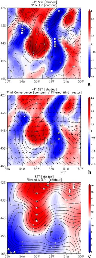
www.nature.com/scientificreports/
In the BMC region, the water masses mixing from both the BC and MC define the western end of the sub-
tropical convergence in the Southwestern Atlantic, a region known for the formation and subduction of South
Atlantic Central Water (SACW). The latter spreads throughout the SWA into subsurface layers. The confluence
generates strong lateral thermal gradients with values ranging from 0.01 °C k m−1 up to 0.08 °C k m−1 3 and is
highly variable in both time and s pace8–11 as it meanders around 38°S12. Also, the coastal region of the SWA is
known to be one of the most important cyclogenesis regions of the atmosphere in the Southern Hemisphere
(SH) with storm tracks eventually reaching the southern and southeastern parts of South America (SA)13,14. The
SST gradient near the southeastern South American coast may play an essential role in cyclogenesis and cyclone
intensification near 35°S14.
On the oceanic mesoscale, both the atmosphere and ocean are highly turbulent. In this context, ocean eddies
occur as entities responsible for across-front mixing and transport of different physical, chemical, biological,
and biogeophysical properties15–18, such as the mixing of tracers, kinetic energy, potential vorticity, phytoplank-
ton concentration, and, particularly iron r edistribution15–17,19. Among the factors producing ocean eddies in
the BMC are the extreme thermal front that produces baroclinic instabilities20, the South American coastline
orientation, and the ocean current reversals15 occurring when the eddies are shed from the main c urrents8,15,21.
The BC reaches its southernmost positions during the austral spring and summer and the warm core eddies are
shed at a yearly rate of seven or more22.
Mesoscale ocean eddies tend to retain the properties of the original currents, thereby exhibiting different
properties relative to their surroundings after shedding. They have characteristic time scales of months and
spatial scales of several-tens to hundreds of kilometers21–23. They are also a source of intrinsic climate variability
by modifying the large-scale circulation, SST, and ocean–atmosphere fl uxes6,24. These eddies also have a large
influence on biogeochemical cycles not only through lateral stirring and m ixing25 but also through the vertical
26
advection of nutrients in and around the eddies , which are easily observed in chlorophyll-a images such as
shown in Fig. 1c. Their surface thermal signature locally affects the overlying atmosphere, where warm (cold)
eddies locally produce positive (negative) turbulent heat flux anomalies and an associated warm, well mixed,
unstable (cool, stratified, stable) M ABL6,27,28. These interactions feed back to affect the eddies themselves, since
they also locally influence near-surface wind, cloud properties, and r ainfall29.
Carbon dioxide ( CO2) is one of the greenhouse gases present in the Earth’s atmosphere and anthropogenic
emissions have increased both atmospheric and oceanic concentrations, thus leading to climate change and
to ocean acidification30–32. In general, tropical oceans are sources of CO2 to the atmosphere, while oceanic
regions at mid to high latitudes absorb atmospheric C O2, thereby being considered as natural sinks of this g as33.
One of the main sinks of CO2 is the ocean, known to absorb approximately one-third of the total anthropo-
genic emissions34,35. The Southern Ocean, which feeds the Malvinas Current, is an especially important sink of
atmospheric CO2. Recent studies, however, reported uncertainties on ocean–atmosphere gas transfer velocity
estimations36 and a decrease in this ocean’s absorption capacity due to increased wind intensity that modulates the
CO2 ventilation from the deep ocean37. In addition, warm core eddies that travel to mid latitudes in the vicinity
of subtropical oceanic fronts can play a role like the tropical ocean and act as a C O2 source to the atmosphere.
This is the case we report here.
However, the physical mechanisms by which oceanic thermal signatures affect the stability of the atmosphere
overlying eddies is still an active field of study. The study presented here sheds light on this topic by offering
comprehensive results based upon rare, in situ observations of one such eddy. In particular, we discuss the ability
of a warm core ocean eddy to modify the physical, dynamic, thermodynamic and CO2 properties of the oceanic
environment where it lives, as well as its impacts on the overlying atmosphere. This type of phenomenon is still
subsampled in this region. Our novel in situ and eddy-covariance turbulent flux data used in this study provides
more understanding of the physical MABL stability mechanisms and ocean–atmosphere fluxes exchanges includ-
ing momentum, heat, and C O 2.
Results
The Antarctic Modeling and Observation System (ATMOS) project, which is part of the Brazilian Antarctic
Program (PROANTAR) sampled a WCE in the BMC region (Fig. 1a) during its first cruise named as ATMOS-
138. We used the Eddy Covariance (EC) method39–43 to measure the air-sea turbulent fluxes of CO2, momentum,
sensible heat, and latent heat. To identify the impact of the eddy on its surrounding environment, such as the
MABL dynamic and thermodynamic characteristics, we used complementary meteorological and oceanographic
in situ data collected during the cruise.
Atmospheric synoptic conditions. Our analysis begins by evaluating the large-scale atmospheric synop-
tic patterns that occurred during the ATMOS-1 cruise sampling period, from 18 to 19 October 2019, as detailed
in Table 1. During most of the eddy-sampling period, the weather was cloudy, with light rain and fog. These
atmospheric conditions were associated with the presence of an extratropical cyclone, which was migrating
eastward and undergoing occlusion along the northern fringe of the WCE study area near the first westernmost
sampling point (Fig. 1a). Around the time we launched our first radiosonde in this area, the sea level pressure in
the central part of the extratropical cyclone was approximately 1006 hPa. The cyclone was located northwest of
the launching position, while a zonally-oriented pressure ridge was situated to the south of the observational site.
This synoptic configuration produced surface winds from the east-northeast during most of 18 October, with
magnitude ranging from 5 to 18 m s −1 (Table 1). Winds with a northerly component promoting warm advection
within the MABL were observed with the first two atmospheric soundings launched in the afternoon. From the
evening of 18 October into the early morning of the following day, the wind direction in the MABL acquired a
southerly component following the zonal displacement of the cyclone center towards the northeast of the study
Scientific Reports | (2021) 11:10648 | https://doi.org/10.1038/s41598-021-89985-9 2
Vol:.(1234567890)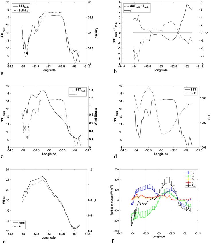
www.nature.com/scientificreports/
Figure 1. Images showing Southwestern Atlantic Ocean and study area. (a) MUR Sea Surface Temperature
(°C) with Reanalysis ERA5 Sea Level Pressure (hPa) showing the study area in a broad view. (b) Same as (a),
but in view zoom of the eddy. (c) Sea Level Anomaly (m) relative to the geoid measured by Altimetry (colors)
and derived absolute geostrophic velocity current vectors (m s-1). (d) Chlorophyll-a concentration (Chl-a in mg
m−3). All data are for 18th October 2019. The white circles denote the Po/V Almirante Maximiano trajectory
while crossing the eddy dipole and the XBTs and radiosondes launching positions. The symbols over the
continent indicate the country names of Brazil (BR), Uruguay (UY) and Argentina (AR). Grid Analysis and
Display System (GrADS), Version 2.2.1.oga.1. http://opengrads.org. MATLAB, Version 9.1.0.441655 (R2016b).
https://www.mathworks.com.
Scientific Reports | (2021) 11:10648 | https://doi.org/10.1038/s41598-021-89985-9 3
Vol.:(0123456789)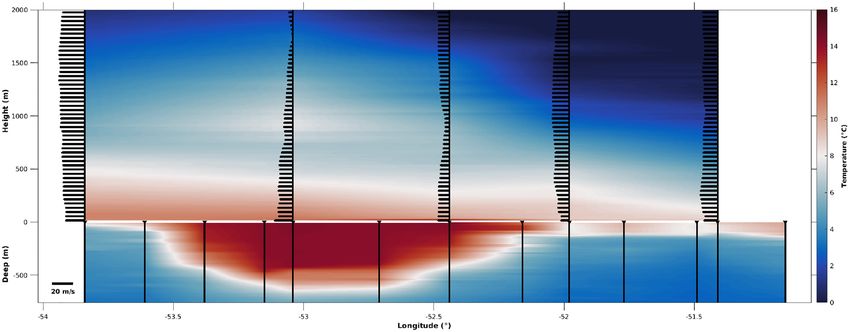
www.nature.com/scientificreports/
MABL
Station Date Local time Longitude (° W) Latitude (° S) SST (°C) Tair (°C) SLP (hPa) RH (%) WS (m s −1) WD (°) (m)
1 18/10/19 10:07 53° 50.57′ 43° 12.20′ 9.5 10.5 1010.3 95 17.9 79 960
2 18/10/19 16:21 53° 02.93′ 44° 03.89′ 14.4 11.0 1008.1 95 15.2 82 790
3 18/10/19 19:40 52° 26.37′ 44° 24.40′ 14.2 15.3 1008.9 95 10.4 154 980
4 18/10/19 23:36 51° 58.99′ 44° 45.95′ 9.0 13.0 1010.3 85 5.0 220 500
5 19/10/19 03:29 51° 24.14′ 45° 06.43′ 8.2 9.0 1010.3 85 9.0 202 750
Table 1. Radiosonde date, time and position of launching. Sea surface temperature (SST), air temperature
(Tair), sea level pressure (SLP), relative humidity (RH), wind speed (WS), direction (WD). T
air and SLP were
measured by ship’s automatic weather station (AWS). SST that was obtained by the ship’s thermosalinographer
and MABL top height that was estimated from radiosondes data.
area. The cyclone continued to exhibit some deepening, with its central pressure dropping to 1002 hPa. In this
final stage of the intensive observing period the surface wind speed varied from approximately 5 to 9 m s −1.
Oceanic synoptic physical and biological conditions. Satellite-derived Sea Level Anomaly (SLA),
SST and chlorophyll-a (Chl-a) concentration data were used to identify the eddies present in the BMC region
and define the ship route before the cruise in order to cross a pair of warm and cold core eddies as shown in
Fig. 1. We clearly identified a well-defined warm core (anticyclonic) eddy, as are typically shed by the Brazil
Current in the BMC (Fig. 1a). Southeast of it, a cyclonic cold core eddy (CCE) was also present (Fig. 1a,b). This
eddy pairing suggests that it may be a dipole system. However, our main focus here is on the WCE, given its
impressive signature and potential role in governing ocean–atmosphere interactions. The analysis of satellite-
derived SST fields shows that the WCE central temperature is about 14 °C, decreasing to 9 °C along its edge.
When reaching the edge of CCE via ship the SST was about 7 °C. This yields a SST difference of approximately
5 °C between the WCE and its border and of roughly 7 °C across the strong thermal front, similar to the ones
seen previously at the BMC front2,3. This marked gradient is responsible for modifying the surrounding oceanic
environment where this WCE is situated as we later demonstrate. The WCE had its center located at 44°S and
52°W with a mean radius of 95 km when observed. These characteristics are similar to a previous WCE analyzed
in this region28. The structure extended north–south for 1.8° and east–west for 2°, as estimated using the SLA
from satellite altimetry (Fig. 1d).
A direct relationship between SST, SLA, and the geostrophic currents derived from SLA can be seen in
Fig. 1c. The WCE exhibited translational velocities reaching 1 m s −1 while the CCE velocities were less than 0.5
m s−1 (Fig. 1c). The lifecycle of a WCE detached from the Brazil Current can last for months with estimated
translational velocities ranging from 5.8 to 7.8 km d ay−1 and, instead of just merging into surround waters by
mixing or diffusion, can be re-assimilated by the parent c urrent21. In our case, the eddy life cycle lasted 86 days
(7 September 2019 to 1 December 2019) after which it was re-assimilated by the Brazil Current.
The WCE also imprinted a profound signal in the chlorophyll-a surface concentration field. The typical
mean Chl-a values over the BC (MC) ranged from 0.015 to 0.5 (0.2 to 0.5) mg m -3 during September and Octo-
ber 201915. In Fig. 1b,d it is evident that SST and Chl-a values at the WCE center are those typically found in
BC waters. This confirms that this eddy was decoupled from the BC and transported its characteristics along
its trajectory, a m echanism44 called eddy trapping. Furthermore, at the WCE periphery (where colder waters
were located) we found higher Chl-a values, reaching 1.5 mg m -3. Similar Chl-a patterns in anticyclonic eddies
in, and to the north of, the Southern Antarctic Circumpolar Current Front were previously observed45. It has
also been observed that submesoscale density fronts (horizontal scale < 10 km) are commonly generated at the
periphery of mesoscale e ddies44,46,47. These submesoscale fronts are characterized by strong vertical ageostrophic
circulation48,49, with upwelling rates reaching 10 m day−1 50–52. Therefore, these regions are potentially an efficient
route for vertical transport of n utrients53. Several studies based upon ocean color data support this idea, reporting
high Chl-a surface concentration close to the periphery of e ddies45,47,54, as also seen in our Fig. 1d.
In our case, the low Chl-a concentration in the WCE core may be due to eddy trapping during its formation,
while the high Chl-a concentration at the borders might be explained by the action of submesoscale processes
(Fig. 1d). Another region with high Chl-a concentration is located northeastward of the WCE, coinciding with
the SST front location (Fig. 1b).
Due to its anticyclonic circulation and consequent eddy-induced Ekman pumping, there is mass convergence
inside the WCE that results in a deepening of the thermocline where the eddy is located (Fig. 2). An increase in Chl-a
concentration (Fig. 1c) of 1.5 mg m−3 up to 4 mg m−3 at very localized spots is seen in the regions where the greatest
SST gradients are located between the WCE and the cold waters around it (e.g. 44°S and 55°W). The same happens
where the CCE is located (Fig. 1a), with a consequent resurgence of nutrient-rich colder waters. The high Chl-a con-
centration seen at the WCE periphery coincides with the climatological October-December Chl-a c oncentration55
of 1.5 mg m −3 associated with the Patagonian Shelf Large Marine Ecosystem (PSLME), one of the most productive
and complex marine regions in the Southern H emisphere56 and located slightly to the west of the WCE.
The vertical structure of our WCE clearly reveals a mixed layer depth of 426 m with temperatures ranging
from 14 °C to 14.2 °C (red line in Fig. 2a). A well-stablished thermocline occurs below it, with temperatures
ranging from 13.9 °C at 430 m to 5 °C at 760 m, as shown in Fig. 2a. Both indicate that this is a barotropic and
well mixed temperature region in the ocean. The opposite is seen when moving from the eddy center towards
its borders, where colder waters are present. This is seen mainly in the CCE (profile 4 and 5 in Fig. 2a). Those
Scientific Reports | (2021) 11:10648 | https://doi.org/10.1038/s41598-021-89985-9 4
Vol:.(1234567890)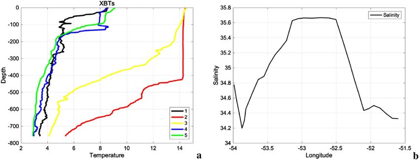
www.nature.com/scientificreports/
Figure 2. Synoptic, in situ measurements taken along Brazilian Navy Polar Vessel (Po/V) Almirante
Maximiano (H-41) route while crossing the eddy. (a) XBT temperature (°C) depth profiles. The numbers in the
legend denote de XBT positions, with 1 being the westernmost position and 5 being the easternmost position.
The number 2 (red) is closest to the eddy core position. (b) Salinity, measured by ship thermosalinographer.
MATLAB, Version 9.1.0.441655 (R2016b). https://www.mathworks.com.
profiles reveal a shallower temperature mixed layer, reaching depths of approximately 100 m. Interestingly, the
temperature-depth profile of station 4 (Fig. 2a) shows an inversion in the water temperature with respect to
the depth near 106 m. There the water temperature decreased to 7.8 °C and below it increased to 8.6 °C at 116
m, and then continued to decrease downward as expected. This inversion can be associated with a subsurface
meandering structure commonly present in oceanic, baroclinic frontal r egions57. Below that we see a shallower
and well-stablished thermocline, with an abrupt temperature decrease from 8.6 °C down to 4.8 °C at 192 m.
Another important characteristic of the WCE is its surface salinity (Fig. 2b), with values ranging from about
34.2 at the borders to about 35.7 at the center of the eddy. This hat shape in the salinity surface profile is typical
of warm core eddies in the BMC region, where lower salinity values are found at the eddy’s periphery where
cold, less saline waters are present. The thermohaline values found inside our WCE confirm that it originated in
a region of mixing between Tropical, Subantarctic, and South Atlantic Central W ater58. Open questions persist
about local processes such as eddy mixing, transport of tracers, and redistribution of other oceanic properties59.
These questions mainly involve the specific theoretical processes and are dependent upon accurate vertical
volume sampling of eddies59.
The WCE life cycle lasted for 86 days, estimated from a sequence of SLA satellite images. This eddy had dimen-
sions of 2.20 1 05 m in the meridional direction, 1.58 1 05 m in the zonal direction and was approximately 350 m
deep, with 15 °C average temperature, approximately, by the time it was sampled by the ship. Those dimensions
indicate this WCE has a volume of 9.55 1 012 m3, with approximately 5.59 1 019 J of heat content excess compared
to its surroundings. This heat content excess is larger compared to the few previous measurements made in the
BMC region11. The net heat transfer from ocean to atmosphere over the eddy was estimated as 7.07 1 017 J, con-
sidering that this excess of heat flux is a function of the eddy area during the sampling day. Our calculations are
novel for this study region over this kind of oceanic mesoscale structures and reveal that approximately 1.3% of
the ocean heat energy excess contained inside the WCE were transferred to the atmosphere, during the sampling
period when our in situ measurements were made.
Oceanic boundary layer and marine atmospheric boundary layer observations. The MABL and
oceanic boundary layer (OBL) vertical profiles are shown in Fig. 3. The following analysis was made in order to
evaluate the MABL static stability that is induced by the SST anomalies present in the ocean, as already described
for the Eastern Equatorial Pacific60, the CBM2,3 and the SWA40. In the well-known vertical mixing mechanism60,
the air buoyancy and turbulence intensity increases over warm waters. As a consequence, the MABL vertical
wind shear is reduced, and stronger winds are generated at the sea surface. This process increases the transfer of
momentum from the atmosphere to the ocean surface thus enhancing oceanic mixing processes and intensifying
ocean–atmosphere fluxes61. An opposite situation is expected over cold waters. Figure 3 shows the MABL and
OBL temperature vertical profiles (°C) taken along the Po/V Almirante Maximiano’s route during 18 October
2019. Wind magnitude vectors, overlaying the temperature profiles, clearly show that over warm waters the
surface and near surface winds are stronger and present a small or non-existent vertical shear. This is a classic
characteristic of a well-mixed and turbulent MABL, reflected also by the air temperature vertical homogeneity,
as shown by the two westernmost atmospheric profiles in the upper half of Fig. 3. However, outside the WCE
beyond its eastern border, the vertical wind shear increases, indicating an increase of the MABL stability and a
decrease of surface wind magnitudes, as shown by the three easternmost atmospheric profiles in the upper half
of Fig. 3. This process is part of the OBL and MABL interplay, where some of the surface oceanic characteristics
Scientific Reports | (2021) 11:10648 | https://doi.org/10.1038/s41598-021-89985-9 5
Vol.:(0123456789)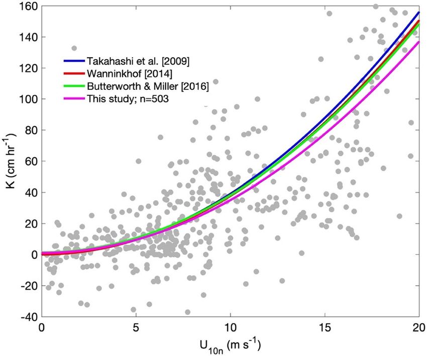
www.nature.com/scientificreports/
Figure 3. Temperature profiles (°C) of the atmosphere and ocean (colors) taken simultaneously by radiosondes
and XBTs along the Brazilian Navy Polar Vessel (Po/V) Almirante Maximiano (H-41) route while crossing the
eddy during 18th October 2019. The lower part of this figure also displays the oceanic sounding positions. Wind
magnitude (m s-1) in vectors is also displayed, superimposed on the air temperature. The vector size reflects the
wind magnitude. MATLAB, Version 9.1.0.441655 (R2016b). https://www.mathworks.com.
Sensor Model Manufacturer Variables sampled Sampling rate (Hz) Height/depth installation (m)
Integrated CO2/H2O CO2 density, H
2O density
Open-path gas analyzer and 3D sonic IRGASON Campbell Scientific 3D wind components air temperature, 20 14.33
anemometer air pressure
Net Radiometer CNR2 Campbell Scientific Net short and long wave radiation 1/60 12.87
Pyranometer CMP3-L Kipp & Zonen Incoming short wave radiation 1/60 15.26
Compass C100 KVH Industries Direction 20 15.2
GPS GPS16X-HVS Garmin Position 20 15.13
3D accelerations and 3D angular
Multi axis inertial sensing system MotionPak II Systron Donner Inertial 20 14.14
velocities
Barometric Pressure Sensor CS106 Vaisala Air pressure 1/60 15
Thermosalinograph SBE45 Sea Bird SSS and SST 1/60 −5
Table 2. Meteorological and oceanic sensors installed on the micrometeorological tower and ship hull during
the ATMOS-1 cruise.
are passed to the lower atmosphere. We need, however, to remark that our westernmost radiosonde (our first
launching) does not show the expected typical behavior of cold waters locally modulating the MABL. We believe
that this finding is associated with the influence of the extratropical cyclone previously described here.
Heat fluxes and radiation balance. Next, we turn our attention to investigate the MABL stability using
surface oceanographic and meteorological measurements in situ. The high-frequency sampling (20 Hz) made
with our micrometeorological tower includes CO2 and water vapor (H2O) gas concentrations, three compo-
nents of wind speed, air temperature (Tair), barometric pressure, ship velocity, position and 3D angular accelera-
tions and angular velocities. Short and long wave radiation measurements were acquired at lower frequency (1
acquisition per minute). SST and sea surface salinity (SSS) were taken from the ship’s thermosalinographer and
hull’s ADCP. More details on the use of the instruments are shown in Table 2. The SST-Tair used here is one of
the criteria for determining the stability of the M ABL2,3,40 and provides an indication of the direction of heat
fluxes typically showing positive (negative) values associated with positive (negative) fluxes from the ocean to
the atmosphere2,3,40. All of our tower sensors were tested and calibrated by the Meteorological Instrumentation
Laboratory of INPE before and after the experiment. Also, all of our measurements taken at high frequency,
including sea level pressure, were in good agreement with the lower frequency data obtained from the ship auto-
matic weather station (AWS), but not shown here.
The measurements clearly show that the WCE exerts a marked presence by modifying the surrounding waters
and providing a large source of heat to the atmosphere, as seen in Fig. 4. The SST at the eddy core was 14 °C
(Fig. 4a), which was 2 °C higher than T air taken on the ship’s bow tower at 16 m height from the sea s urface62 and
measured at the same times and locations. This is quantified by the strong vertical thermal difference (SST-Tair)
seen on the time series in Fig. 4b.
Scientific Reports | (2021) 11:10648 | https://doi.org/10.1038/s41598-021-89985-9 6
Vol:.(1234567890)www.nature.com/scientificreports/
Figure 4. Synoptic, in situ measurements taken along Brazilian Navy Polar Vessel (Po/V) Almirante
Maximiano (H41) route while crossing the eddy. (a) SSTbulk (°C) and salinity. (b) Stability parameters, ζ and
SST—Tair (°C). (c) SSTbulk (°C) and wind stress (N m-2). (d) SSTbulk(°C) and sea level pressure (hPa). (e) Wind
speed magnitude and friction velocity (u*), both in m s -1. (f) Components of net heat flux (Qnet), short and
long wave radiation (Sw and Lw), latent and sensible heat fluxes (Ql and Qs, both measured by eddy covariance)
in W m-2. The bars in (f) are the standard error oriented up for visual clarity representing 95% confidence
interval. However, they must be interpreted both up and down. All information is derived from the ship-borne
meteorological data. MATLAB, Version 9.1.0.441655 (R2016b). https://www.mathworks.com.
Positive values of SST-Tair define an unstable MABL and the larger this difference is, the more unstable the
MABL is. A second MABL stability parameter evaluated here is the Monin–Obukhov stability parameter (ζ ),
shown in Fig. 4b. This parameter tends to corroborate our SST-Tair series, with negative values over the region
Scientific Reports | (2021) 11:10648 | https://doi.org/10.1038/s41598-021-89985-9 7
Vol.:(0123456789)www.nature.com/scientificreports/
that SST-Tair is positive. The parameter ζ is a function of the scaling parameter L defined as the Obukhov length
and indicating the height of the boundary layer where the buoyancy factors dominate compared to the turbulent
vertical transport caused by the w ind63. Negative values of ζ indicate a MABL that is statically unstable while
positive values mean statically stable conditions.
Strong surface wind speed was observed on the westernmost side of the WCE, reaching a maximum value
over the warmer waters of the WCE core (Fig. 4e). Wind speed minima are observed over the cold waters along
the eastern side of the WCE, at the CCE center. It is interesting to note that the WCE advects and retains the BC
thermohaline properties, showing higher SSS values of 35.6. These positive values of SST-Tair (Fig. 4b) and higher
SSS values (Fig. 4a) span a considerable area of the WCE’s surface. Lower SLP values coincided with higher SST
values (Fig. 4d), demonstrating that the lower atmosphere was influenced by the WCE’s local modulation. In
order to substantiate this, we complement our study using the ERA5 reanalysis (Fig. 5). Discussion follows in
the last paragraph of this section.
This WCE role as a heat source to the atmosphere is also clearly noticed in the heat balance presented in
Fig. 4f,based on our in situ observations. The spatio-temporal variability of net heat flux (Qnet) indicates the
WCE net heat contribution, where positive values mean the WCE induces a heat flux directed from the ocean to
the atmosphere. The turbulent heat fluxes are proportional to the temperature and specific humidity differences
between the air and the sea surface, as well as to the wind magnitude and the stability coefficient. The positive
contribution of the sensible ( Qs) and latent ( Ql) heat fluxes estimated by the Eddy Covariance (EC) method and
the thermal longwave radiation ( Lw) are also seen over most of the area of the WCE. As previously described,
during the whole sampling period the sky was cloudy and this is reflected in the relatively low diurnal net short
wave radiation ( Sw) fluxes. The mean EC heat fluxes are also corroborated by the bulk calculation of fl uxes64, as
can be verified in the supplementary material presented in Figure A1.
The impressive case of eddy-induced MABL modulation presented here using observational data was also
verified by an independent reanalysis data. The independent ERA5 SST data, although having lower resolution
in respect to satellite estimates (Figure A2a), clearly showed a well-defined pattern associated with our eddy as
also seen in Fig. 1. The reanalysis wind stress (τ ) overlays SST in that figure to show that the wind magnitude
increases over warmer waters. Moreover, when τ components are filtered and the higher frequency modes are
retained and displayed (Supplementary Figure A2b), the effect of the wind acceleration (deceleration) over
warmer (colder) waters is highlighted even more, corroborating what was already reported for other regions of
the world ocean25. The atmospheric surface modulation by the WCE is strong enough to make its effects noticed
in higher levels of the MABL column of air overlying it (Supplementary Figure A2a and A2b). The ascendant
air movement is coincident with the region where higher SST values are located and a higher MABL top occurs.
Conversely, descendant air movement is noticed where lower SST values and MABL top heights occur. These
results, together with our in situ atmospheric vertical profiles (Fig. 3) clearly demonstrate the capacity of the
WCE to influence the MABL vertical structure. Reanalysis data also showed that the MABL height approximately
varies from 650 m over warmer waters to 450 over colder waters. However, the reanalysis underestimates the
MABL height, compared to what was estimated through radiosondes. The height was approximately 960 m, 790
m and 980 m over warmer waters and 500 m and 750 m over colder waters (Table 1).
ERA5 data were also used to investigate the role of WCE on the local modulation of the overlying atmosphere.
Besides the vertical mixing m echanism60 already explored earlier in this study, another mechanism can explain
the surface wind modulation by SST. This mechanism occurs in regions of strong SST gradients and is known
as the pressure adjustment mechanism65. It relates the Laplacian of the SLP (∇ 2 SLP) and SST with the reversed
sign (−∇ 2 SST) with the surface wind c onvergence66. In this way, it is possible to isolate the WCE effects on the
MABL modulation from background effects caused by the large-scale atmospheric systems. During the WCE
life cycle, we observed that for the 10-day period ranging from 15 to 25 October 2019 the eddy remained almost
stationary in the location where it was sampled by the ship during the ATMOS-1 campaign. We used this period
to calculate the mean fields of SST, SLP, and wind magnitude at 10 m and then estimate the − ∇ 2SST, ∇ 2 SLP and
wind convergence fields (Fig. 5a,b). Figure 5b also shows the filtered wind field at 10 m. There we can see that the
wind diverges in regions with lower SST and converges in regions with higher SST. Furthermore, we observed
positive (negative) values of ∇ 2 SLP in regions with positive (negative) values of − ∇ 2SST (Fig. 5a). This relation-
ship indicates that the surface wind convergence occurring over the WCE (Fig. 5b) is associated with the pressure
adjustment mechanism induced by the SLP gradient, observed between the WCE region (lower SLP) and the
neighboring regions (cold waters, higher SLP—Fig. 5c). Note that in our case a geographical shift is observed in
the convergence area with respect to the eddy center, which is a feature that was also observed in similar studies67.
Carbon dioxide analysis. We finish our data analysis using our high-frequency data to show how our
WCE effectively modified the surrounding ocean–atmosphere C O2 fluxes. To our knowledge this kind of in situ
observation is unique in the Southwestern Atlantic Ocean. This region supports one of the largest CO2 sinks of
the global ocean. Previous s tudies68 reveal that the region has an annual average, ocean–atmosphere difference
of the CO2 partial pressure (ΔpCO2) of − 31 atmµ. The average CO2 ocean–atmosphere flux is − 3.7 molm m−2
day−1 (negative indicates a sink where the ocean absorbs CO2 from the atmosphere). However, the Southwestern
Atlantic is a transition region to the Southern Ocean, where many warm eddies are shed from the BC to colder
waters with the ability to change the environment they transit by carrying physical, chemical and biological
characteristics from their region of origin28,59,61. Our measurements displayed in Fig. 5 clearly show that the
analyzed WCE carries the original Brazil Current characteristics further southwards than this current alone
is capable of doing. The waters inside the eddy are warmer (Fig. 1a), saltier (Fig. 2b) and depleted of nutrients
(Fig. 1d). During the ATMOS-1 campaign, the wind direction (Table 1) varied from northeast to southwest (first
and third quadrants) causing different atmospheric advection conditions. The ocean–atmosphere CO2 fluxes
Scientific Reports | (2021) 11:10648 | https://doi.org/10.1038/s41598-021-89985-9 8
Vol:.(1234567890)www.nature.com/scientificreports/
Figure 5. Maps of 10-day-averaged surface atmospheric and oceanic variables from ECMWF ERA5 reanalysis.
a) negative Laplacian of Sea Surface Temperature (− ∇ 2 SST 10−9 K m-2) is shaded and Sea Level Pressure (∇ 2
SLP 10−9 Pa m-2) is contoured. (b) Laplacian of Sea Surface Temperature (- ∇ 2 SST 10−9 K m-2) is shaded, wind
convergence (∇w 10–6 s-1) is contoured and high-pass-filtered field of wind (vectors). c) Sea Surface Temperature
(°C) is shaded and high-pass-filtered field of Sea Level Pressure (hPa) is contoured. Grid Analysis and Display
System (GrADS), Version 2.2.1.oga.1. http://opengrads.org.
Scientific Reports | (2021) 11:10648 | https://doi.org/10.1038/s41598-021-89985-9 9
Vol.:(0123456789)www.nature.com/scientificreports/
Figure 6. Atmospheric in situ C O2 fluxes measured by Eddy Covariance method along Brazilian Navy Polar
Vessel (Po/V) Almirante Maximiano (H-41) route while crossing the eddy. (a) CO2 fluxes (µmol m-2 s-1) and
stability parameter ζ 102. (b) CO2 fluxes (µmol m-2 s-1) and stability parameter SST—Tair (°C). The error bars are
the standard error and are oriented up. The bars are the standard error oriented up for visual clarity representing
95% confidence interval. However, they must be interpreted both up and down. MATLAB, Version 9.1.0.441655
(R2016b). https://www.mathworks.com.
measured during the field campaign tend to reflect this environment and follow the MABL stability variability.
The parameter ζ and values of SST-Tair provided indications of how turbulent the atmospheric layer was near
the ocean surface. There is a sign change of these parameters due to cold advection associated with both cyclone
transition and the reduction of SST at the end of the ship’s transect during ATMOS-1. As a result, positive and
lower CO2 fluxes were then observed. This is also corroborated by comparing our CO2 flux measurements with
both atmospheric stability parameters ζ and SST-Tair, shown in Fig. 6. Ocean–atmosphere CO2 fluxes were posi-
tive (from the ocean to the atmosphere) in the region of larger SST anomalies and MABL instability, where ζ was
negative (Fig. 6a) and SST-Tair (Fig. 6b) and − ∇ 2 SST (Fig. 4f) were both positive. In conclusion, the effect of the
WCE studied here was to modify the typical behavior of the Southwestern Atlantic Ocean, an ocean expected
to be a CO2 sink.
In order to assess the quality of the CO2 fluxes calculated in this study, the CO2 ocean–atmosphere transfer
velocity coefficient (K) was computed and compared to some classic values found in the l iterature69,70 and with
a more recent one developed for the Southern O cean36 (Fig. 7). We found a quadratic adjustment (K = 0.34
U10n2 – 0.32 U10n + 0.94) between the CO2 transfer coefficients and the neutral wind speed collected at 10 m
(U10n) during the cruise. For U10n less than 7 m s−1 our curve showed a good agreement with previous studies.
However, for U10n greater than 7 m s−1, the K values were lower than the curves used for comparison. Even so, it
is possible to observe that the K curve was able to satisfactorily represent the expected behavior. When the wind
speed is zero then K = 0.94 cm h−1, which is higher than the studies used here for comparison. We can associate
this discrepancy with processes such as internal turbulence at the ocean s urface36 or the biological activity that
is characteristic of this region.
Discussion
In summary, ocean eddies play a fundamental role in transporting and mixing properties between regions with
heterogeneous characteristics. In this observational turbulent flux study in the Southwestern Atlantic Ocean,
we presented and highlighted the ability of a warm core ocean eddy shed from the Brazil Current to modify
both the ocean and the surrounding atmosphere. Since 2012 the Southwestern Atlantic Ocean has been sampled
during research cruises using the Eddy Covariance (EC) method to directly measure the ocean–atmosphere
heat, momentum, and gas fluxes in combination with more traditional methods of observing the ocean and the
atmosphere from s hips2,3,40. The present study shows that the lateral SST gradients produced by the presence
of a WCE in cold waters extensively affect the MABL stability and that the eddy effects may cross the top of the
MABL and reach the troposphere (Supplementary Figure A3).
There is a lively debate about the mechanisms by which the atmosphere near the ocean surface may become
unstable in various regions of the w orld3,61,66,71–73. The pressure adjustment mechanism, explained above, is not
easy to identify using observational studies due to the sparse resolution that is often intrinsic to the data set.
However, the good spatio-temporal quality of our observational data and the support of complementary (ERA5)
reanalysis data allowed depiction of the effectiveness of the pressure adjustment m echanism66,74. The mechanism
causes a wind convergence over warm-core eddies and a wind divergence over cold-core eddies, measured
through the link between the SST to the SLP Laplacian fields. Concomitantly, the stability parameters determined
from the ocean–atmosphere temperature difference and the Monin–Obukhov stability parameter (ζ ) together
diagnose a MABL static stability induced by the SST anomalies2,3,40,60. The increased (diminished) vertical mix-
ing is associated with a more unstable (stable) MABL over warmer (colder) waters. These sudden changes in
Scientific Reports | (2021) 11:10648 | https://doi.org/10.1038/s41598-021-89985-9 10
Vol:.(1234567890)www.nature.com/scientificreports/
Figure 7. Relationship between the C O2 transfer velocity coefficient and the neutral wind speed at 10 m
calculated from the data collected in this experiment. The quadratic fitted curve K = 0.34.U10n2 – 0.32 U10n + 0.94
with r2 = 0.75 is represented by the magenta line. The blue, red and green curves represent the C O2 transfer
coefficient obtained in the literature36,69,70. MATLAB, Version 9.1.0.441655 (R2016b). https://www.mathworks.
com.
the SST and the increase (decrease) of vertical turbulent mixing related to the large (small) ocean–atmosphere
temperature differences establish a decreased (increased) atmospheric vertical wind shear.
The EC is considered the best method to quantify the ocean–atmosphere C O2 fluxes because its uncertainties
are of the order of only 5%75. These uncertainties are much smaller than those associated with the bulk methods
that use (uncertain) transfer coefficients. From this technique, our direct unprecedented CO2 measurements
indicate an eddy contribution of 0.3 + /− 0.04 molm m−2 day−1 to the atmosphere over the ATMOS-1 sampling
period. If one considers its entire life cycle of about three months, then the amount of C O2 that may be trans-
ferred to the atmosphere can reach values of 25.8 ± 3.56 mmol m -2. The ocean–atmosphere C O2 transfer velocity
coefficient, computed with our data and quadratically fitted to wind speed, yielded good performance by agree-
ing with K determined in other CO2 studies36,69,70, as shown in Fig. 7. Warm core eddies commonly found in
the Southwestern Atlantic Ocean, like the one studied here, therefore are important natural contributors to the
atmospheric carbon budget throughout their respective life cycles.
This study increases our understanding of how a mesoscale warm core ocean eddy affects its surrounding
environment. We conclude that the particular eddy studied here actively modified both the physical and the CO2
exchanges between the ocean and the atmosphere in the Southwestern Atlantic Ocean. This indicates a need for
further investigating the effect of the overall eddy “population” over time as they affect the atmosphere overlying
the Southwestern Atlantic and throughout the world ocean.
Data and methodology. All in situ data were collected on board the Brazilian Navy Polar Vessel (Po/V)
Almirante Maximiano (H-41) during the ATMOS-1 cruise. This paper presents and discusses these novel and
independent high-frequency measurements of heat, momentum, and CO2 fluxes taken onboard the ship.
The study region is located in the Southwestern Atlantic Ocean near the BMC region. During the period
from 18 to 19 October 2019, the ship crossed a train of both warm and cold core eddies (Fig. 1). While crossing
the study region, many oceanographic and meteorological observations were performed. During the ATMOS-1
cruise, a total of six Expendable Bathy-Thermographs (XBTs) were deployed at the same locations where six
radiosondes were launched (Table 1). The oceanic sampling was complemented by 8 CTD (Conductivity, Tem-
perature, Depth) stations. Unfortunately, the CTD castings were not synchronized in time with the atmospheric
measurements; instead, they were performed during the two following days, when the ship crossed back along
the same trajectory. The reason for that was to minimize the effects of possible changes in the large-scale atmos-
pheric synoptic patterns on modifying our in situ data due to non-local effects. Recall that we aimed primarily
to use the ocean–atmosphere measurements made on the WCE to investigate its potential to locally change the
atmosphere immediately above it (Fig. 3). The applied methodology here is similar to that used in our previous
work2,3,40. At port, a micrometeorological tower was installed on the bow of Po/V Almirante Maximiano follow-
ing previous m ethodology40–43 with different sensors able to collect ocean–atmosphere turbulent flux data of
momentum, latent and sensible heat, CO2 and water vapor. This is based on Eddy Covariance (EC) methodology
and used a sampling frequency of 20 Hz in order to obtain 30-min averaged fl uxes40–43. Surface radiation data
were also collected using the micrometeorological tower for computing ocean–atmosphere radiation fluxes.
All data presented in Figs. 4 and 6 were resampled to 30-min intervals. All oceanographic and meteorological
sensors and main characteristics of use are shown in Table 2. The net surface heat flux (Qnet ) was obtained using
the previously computed ocean–atmosphere heat fluxes and the radiation components using the expression:
Scientific Reports | (2021) 11:10648 | https://doi.org/10.1038/s41598-021-89985-9 11
Vol.:(0123456789)www.nature.com/scientificreports/
Qnet = Sw + Lw + Ql + Qs (1)
where Sw is the net shortwave radiation, Lw is the net longwave radiation, Ql and Qs are latent and sensible heat
fluxes, respectively.
The ocean–atmosphere C O2 flux estimates presented here refer to the total emission of the WCE during the
period of its sampling (Fig. 5). It represents 12 h of sampling summing up to 157.2 molµ m−2 s−1. When extrapo-
lated to a daily emission, we arrive at 0.3 + /- 0.04 molm m−2 day−1. This same estimate was then multiplied by the
estimated life of this eddy (86 days) resulting in a total of 25.8 + /− 3.56 molm m−2. We regard this estimate as, to
our knowledge, the first approximation ever made to represent the total emission of CO2 produced by a warm
core eddy into the atmosphere in the Southwestern Atlantic Ocean during a typical eddy life span.
The ocean–atmosphere transfer velocity of C O2 is obtained through the relationship between variables of these
two environments according to the expression F CO2 = K Sco2 ΔpCO2. Where FCO2 is the C O2 flux (mmol m −2
day ) obtained from the EC, K (cm ) is the gas transfer velocity coefficient and is directly related to the wind
−1 −1
speed69,70 and was adjusted to Schmidt’s number of 660. Sco2 (mol m−3 atm−1) is the CO2 solubility coefficient
(Weiss, 1974) in seawater, using the sea temperature and salinity sampled by the ship’s thermosalinographer that
was available. The ΔpCO2 (μatm) is the difference between the partial pressure of CO2 between the ocean (pCO2w)
and the atmosphere (pCO2a). The pCO2w was obtained from the climatological fi elds69 and pCO2a from a LI 7000
closed-path CO2 analyzer installed at the ship’s bow. A total number of 503 (out of 1473) C O2 flux intervals were
use in the K calculation, after an EC quality control procedure. These data were obtained during 31 days of cruise
in the Southwest Atlantic region and in the Southern Ocean from 3 transits of the Drake Passage between October
6th and December 2nd. Using these data, the quadratic equation K = 0.34.U10n2 – 0.32 U10n + 0.94 with r2 = 0.75
that describes the relationship between K and the neutral wind speed at 10 m ( U10N) was found.
Satellite data were also used in this study. The Group for High Resolution Sea Surface Temperature (GHRSST)
Level 4 analysis derived from the Multi-scale Ultra-high Resolution (MUR) sensor was used. This is a merged,
multi-sensor satellite and in situ SST analysis product with spatial resolution of 0.01° latitude/longitude and daily
temporal resolution provided by the Jet Propulsion Laboratory (http://p odaac.j pl.n
asa.g ov). The sea level anomaly
(SLA) used here is the sea surface height above or below the mean sea surface height relative to the period of 1993
to 2012. These are daily data based on multi-mission altimeter satellite gridded SLA product, and distributed
at level 4, 0.25º latitude/longitude resolution by the European Copernicus Marine Environment Monitoring
Service (http://marine.copernicus.eu). The surface geostrophic currents are also derived from this same data set.
Our in situ data analysis was complemented with the European Centre for Medium-Range Weather Forecasts
(ECMWF) reanalysis data set ERA5 (http://www.ecmwf.int). ERA5 represents the newest version of hourly
estimates of a large number of atmospheric, land, and oceanic climate variables. The surface (pressure level) data
covers the globe with 0.1º (0.25º) latitude/longitude horizontal resolution. The reanalysis is catalogued on 37
pressure levels in the vertical. Using the laws of physics by means of a 4-D variational data assimilation technique
a vast number of observations are combined with model outputs.
In order to retain the smaller-scale signal contained in ERA5 data, we smooth the variable fields using a
successive moving window (spatial) filter with 3 × 3 grid point size that is subtracted from the total field. Many
studies have used space–time filters for this purpose24,76,77. Our choice, although a simplified spatial filtering
strategy yielded in consistent results since we were able to see in our maps the expected spatial coincidence
between the mesoscale SST features present in our study area and the wind stress (Figure A2b), the surface
wind at 10 m height (Fig. 5b), and SLP (Fig. 5c). The same filtering technique was applied on the vertical profiles
shown in supplementary Figure A3.
The calculation of the heat content in the eddy is an important estimate because it allows us to know how
much heat is transported by the eddy during its transit. In this case, the properties originating in the Brazil
Current end up being transported southwards to the Subtropical Front. This heat energy is available for both
contributing to interior ocean processes, such as water mass mixing, and modifying the lower atmosphere.
However, the eddy volume, which is the basic measure to all later estimates, is not easy to be precisely calculated.
Here we assumed an ellipsoid format for our WCE11. We determined the structure’s mean diameter in the zonal
and meridional directions from the SLA satellite image of 18 October 2019. The WCE surface area can then be
calculated as:
Ae = dx 2 · dy 2 · π (2)
where Ae is the eddy area, and dx = 158 × 103 m and dy = 220 × 103 m are the eddy’s zonal and meridional diam-
eters, respectively .
Using our in situ XBT data, we estimated a mean depth of 350 m for the WCE. The eddy volume (Ve ) is then
obtained as follow:
Ve = Ae .de (3)
The de is mean depth of the WCE. The eddy heat content (OHC e ) is then obtained by:
OHC e = ρ.cp .Ve .(Tw − Tc ) (4)
where ρ is the mean water density inside the eddy, cp is the specific heat capacity of the water at the sea surface,
and Ve is the eddy’s volume. Tw and Tc (K) are the mean warmer water surface temperature inside the WCE and
colder water temperature outside the eddy, respectively. This method of calculation allows us to quantify the
WCE heat content excess compared to its surroundings, termed here as OHC e.
Scientific Reports | (2021) 11:10648 | https://doi.org/10.1038/s41598-021-89985-9 12
Vol:.(1234567890)www.nature.com/scientificreports/
A similar calculation was performed aiming to obtain the integrated excess of heat transferred from ocean
to atmosphere, which is not trivial since the determination of the height at which the heat fluxes approach zero
above the surface boundary layer (SBL) remains a key p roblem78,79. This methodology was previously used for
estimates made at fixed locations over l and79. In our case, however, the ship observations were performed with
both time and space varying. As a consequence, the result cannot be the heat flux, but rather the heat excess
transferred from the eddy surface to the atmosphere during the ATMOS-1 c ruise78. The net heat energy trans-
ferred from the WCE to the atmosphere is the difference between the measurements performed over the warm
(in Eq. 5, Qnet_w ) and cold water (in Eq. 5, Qnet_c ). Those estimates were obtained from Eq. 1 and chosen from
Fig. 4f, where Qnet_w = 160 W m -2 and Qnet_c = − 100 W m-2.
(5)
Tot e = Qnet_w − Qnet_c .Ae .Et
and
HE net = (Tot e .100)/OHC e (6)
where Tot e is the net heat energy available for transfer from the WCE to the atmosphere. Et is assumed to be 1
day. Finally, we calculated HE net as a fraction of net energy heat transferred to the atmosphere.
Received: 24 September 2020; Accepted: 26 April 2021
References
1. Tokinaga, H., Tanimoto, Y. & Xie, S.-P. SST-induced surface wind variations over the Brazil-Malvinas confluence: Satellite and
in situ observations*. J. Clim. 18, 3470–3482 (2005).
2. Pezzi, L. P. et al. Ocean-atmosphere in situ observations at the Brazil-Malvinas confluence region. Geophys. Res. Lett. 32, 2–5.
L22603, https://doi.org/10.1029/2005GL023866(2005).
3. Pezzi, L. P. et al. Multiyear measurements of the oceanic and atmospheric boundary layers at the Brazil-Malvinas confluence region.
J. Geophys. Res. Atmos. https://doi.org/10.1029/2008JD0li379 (2009).
4. Acevedo, O. C., Pezzi, L. P., Souza, R. B., Anabor, V. & Degrazia, G. A. Atmospheric boundary layer adjustment to the synoptic
cycle at the Brazil-Malvinas Confluence, South Atlantic Ocean. J. Geophys. Res. Atmos. D22107, https://doi.org/10.1029/2009J
D013785. 115 (2010).
5. Camargo, R., Todesco, E., Pezzi, L. P. & Souza, R. B. Modulation mechanisms of marine atmospheric boundary layer at the Brazil-
Malvinas Confluence region. J. Geophys. Res. Atmos. 118, 1–15, https://doi.org/10.1002/jgrd.50492. 118 (2013).
6. Souza, R.; Pezzi, L.; Swart, S.; Oliveira, F.; Santini, M. Air-Sea Interactions over Eddies in the Brazil-Malvinas Confluence. Remote
Sens. 2021, 13, 1335. https://doi.org/10.3390/rs13071335
7. Gordon, A. L. Brazil-Malvinas Confluence-1984. Deep Sea Res. Part A Oceanogr. Res. Pap. 36, https://doi.org/10.1016/0198-
0149(89)90042-3.(1989).
8. Legeckis, R. & Gordon, A. L. Satellite observations of the Brazil and Falkland currents- 1975 1976 and 1978. Deep Sea Res. Part A
Oceanogr. Res. Pap. 29, 375–401 (1982).
9. Olson, D. B., Podestá, G. P., Evans, R. H. & Brown, O. B. Temporal variations in the separation of Brazil and Malvinas Currents.
Deep Sea Res. Part A Oceanogr. Res. Pap. 35, 1971–1990 (1988).
10. Reid, J. L., Nowlin, W. D. & Patzert, W. C. On the characteristics and circulation of the Southwestern Atlantic Ocean. J. Phys.
Oceanogr. 7, 62–91 (1977).
11. Souza, R. et al. Multi-sensor satellite and in situ measurements of a warm core ocean eddy south of the Brazil-Malvinas Confluence
region. Remote Sens. Environ. 100, 52–66 (2006).
12. Gordon, A. L. Interocean exchange of thermocline water. J. Geophys. Res. 91, 5037 (1986).
13. Hoskins, B. J. & Hodges, K. I. A new perspective on Southern Hemisphere storm tracks. J. Clim. 18, 4108–4129 (2005).
14. Gramcianinov, C. B., Hodges, K. I. & Camargo, R. The properties and genesis environments of South Atlantic cyclones. Clim. Dyn.
53, 4115–4140 (2019).
15. Garcia, C. A. E., Sarma, Y. V. B., Mata, M. M. & Garcia, V. M. T. Chlorophyll variability and eddies in the Brazil-Malvinas Conflu-
ence region. Deep. Res. Part II Top. Stud. Oceanogr. 51, 159–172 https://doi.org/10.1016/j.dsr2.2003.07.016. (2004).
16. Frenger, I., Münnich, M. & Gruber, N. Imprint of Southern Ocean mesoscale eddies on chlorophyll. Biogeosciences 15, 4781–4798
(2018).
17. Ellwood, M. J. et al. Distinct iron cycling in a Southern Ocean eddy. Nat. Commun. 11, 1–8 (2020).
18. Dong, C., McWilliams, J. C., Liu, Y. & Chen, D. Global heat and salt transports by eddy movement. Nat. Commun. 5, 1–6 (2014).
19. Ivchenko, V. O., Danilov, S. & Olbers, D. Eddies in numerical models of the Southern Ocean 177–198. https://doi.org/10.1029/
177GM13 (2008).
20. Garzoli, S. & Simionato, C. Baroclinic instabilities and forced oscillations in the Brazil/Malvinas confluence front. Deep Sea Res.
Part A. Oceanogr. Res. Pap. 37, 1053–1074 (1990).
21. Souza, R. B. & Robinson, I. S. Lagrangian and satellite observations of the Brazilian Coastal Current. Cont. Shelf Res. 24, 241–262
(2004).
22. Lentini, C. A. D., Olson, D. B. & Podestá, G. P. Statistics of Brazil current rings observed from AVHRR: 1993 to 1998. Geophys.
Res. Lett. 29, NO 16,https://doi.org/10.1029/2002GL015221 (2002).
23. Williams, R. G., Wilson, C. & Hughes, C. W. Ocean and atmosphere storm tracks: The role of eddy vorticity forcing. J. Phys.
Oceanogr. 37, 2267–2289 (2007).
24. Small, R. J., Bryan, F. O., Bishop, S. P. & Tomas, R. A. Air-sea turbulent heat fluxes in climate models and observational analyses:
What drives their variability?. J. Clim. 32, 2397–2421 (2019).
25. Chelton, D. B., Gaube, P., Schlax, M. G., Early, J. J. & Samelson, R. M. The influence of nonlinear mesoscale eddies on near-surface
oceanic chlorophyll. Science. 334, 328–332 https://doi.org/10.1126/science.1208897. (2011).
26. Yoder, J. A., Doney, S. C., Siegel, D. A. & Wilson, C. Study of marine ecosystems and biogeochemistry now and in the future:
Examples of the unique contributions from space. Oceanography 23, 104–107 (2010).
27. Villas Bôas, A. B., Sato, O. T., Chaigneau, A. & Castelão, G. P. The signature of mesoscale eddies on the air-sea turbulent heat fluxes
in the South Atlantic Ocean. Geophys. Res. Lett. 42, 1856–1862. https://doi.org/10.1002/2015GL063105. (2015).
28. Leyba, I. M., Saraceno, M. & Solman, S. A. Air-sea heat fluxes associated to mesoscale eddies in the Southwestern Atlantic Ocean
and their dependence on different regional conditions. Clim. Dyn. 49, 2491–2501 (2017).
Scientific Reports | (2021) 11:10648 | https://doi.org/10.1038/s41598-021-89985-9 13
Vol.:(0123456789)You can also read