Mobile Money and Financial Resilience: Overcoming Economic Shocks Through Digital Financial Technology
←
→
Page content transcription
If your browser does not render page correctly, please read the page content below
Mobile Money and Financial Resilience:

Overcoming Economic Shocks Through Digital

           Financial Technology

                            by

                 Phoebe Jane Block, BBA

            Thesis Advisor: Ariel Shwayder, PhD
A thesis submitted in fulfillment of the requirements of the
Michigan Ross Senior Thesis Seminar (BA 480), April 22nd, 2022.

                                                                  2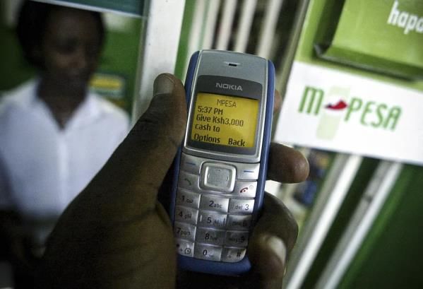
Acknowledgements

        To every educator that I’ve had the pleasure of learning from during the past 17 years:
Thank you for teaching me, encouraging me, challenging me, and mentoring me. There is
nothing more commendable than dedicating your life to the improvement of others. I only wish
to put back into the world every ounce of effort that you’ve invested in me.

        To the friends I’ve made along the way:
Thank you for loving me, supporting me, and growing alongside me. Independent research is the
furthest thing from independent and getting to know you all has been my favorite part of the
journey.

        To my loved ones:
Thank you for listening since the beginning. Thank you for always being there. Thank you for
being the light on the dark days. Thank you for making great days the best days. Having all of
you in my corner makes the largest mountains seem like mole hills.

       To Jack:
Thank you for being the best sibling, friend, and mentor that I could ever ask for. Thank you for
always answering the phone and saving the day. Thank you for always believing and never
doubting. Thank you for pushing me further. I love and admire you so much.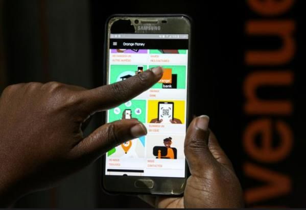
Abstract
        Mobile money has been touted as an opportunity to step toward formal financial
inclusion in developing countries around the world, especially for those traditionally financially
excluded. To further understand the impact of mobile money on those who adopt it, this study
conducts a three-part meta-analysis to test the relationship between mobile money and long-term
financial behaviors. The first part of the meta-analysis summarizes previous studies on mobile
money as it relates to saving, borrowing, and economic stability. The second part uses regression
models to understand how mobile money is related to saving and borrowing propensity using
nationally representative survey data from 9 countries with 60,375 individual observations. The
third part analyzes additional variables relating to coping behaviors during financial crises,
reinforcing findings from the regression models and past studies. Results suggest that having a
mobile money account increases saving propensity by 21% and increases borrowing propensity
by 10% on average. Beyond this, findings from this study suggest a positive relationship between
saving stock and mobile money use as well as a positive relationship between the amount
borrowed and mobile money use. The validity of these findings is solidified by mobile money
users being 5.8% more likely to use formal coping mechanisms during financial crises when
compared to non-mobile money users. From these findings in Africa, Asia, and the Caribbean, it
is possible to hypothesize more broadly about the outcomes of mobile money as it relates to
overcoming economic shocks. These findings are especially relevant given the recent use of
mobile money to distribute stimulus funds during the COVID-19 pandemic.

                                                                                               vii
Contents
Introduction pg 1
What is mobile money? pg 1
Transaction costs and mobile money pg 4
What is financial inclusion? pg 5
Mobile money and financial inclusion pg 6
Statement of the Problem pg 8
Justification of the Problem pg 9
Theoretical Framework pg 11
Defining financial resilience pg 11
Cited barriers to access pg 3
Literature Review pg 14
What are the benefits to financial inclusion? pg 14
Empirical evidence from other countries pg 15
Methodology pg 21
Models pg 21
Instrument rationale pg 23
Descriptive analysis pg 27
Assumptions and Limitations pg 28
Results pg 30
Saving propensity pg 30
Borrowing propensity pg 34
Saving stock and total debt pg 37Coping mechanisms pg 40
Discussion pg 44
Saving pg 44
Borrowing pg 45
Coping mechanisms pg 46
Policy Implications pg 48
Incentives and mandates pg 48
Lowering barriers to account ownership pg 49
Area for Future Research pg 51
Conclusion pg 53
Appendix pg 54
References pg 60
2Introduction
As climate change progresses, global geopolitical relationships become more tense, and
public health systems strain, economic shocks are becoming the new norm. Around the world,
these frequent financial crises challenge cash-based economies, disrupting the ability to
physically transact. At the same time, the digital transformation over the past 30 years has
created tools to help combat these shocks. In the same way that telehealth has revolutionized
access to healthcare during the pandemic, digital financial technologies have the potential to
improve access to financial resources. Mobile money, which is one of the most easily accessible
digital financial technologies, may be the key to improving financial wellbeing before, during,
and after a financial crisis.
What is mobile money?
Mobile money is most broadly defined as “a service in which the mobile phone is used to
access financial services” (Mobile money definitions July 2010 - GSMA, 2010). More
specifically, the type of mobile money that this thesis investigates is a type of account that a user
can access even if they don’t have an existing bank account. These types of accounts require a
SIM card or a cell phone number, and are common across Africa, Asia, and the Caribbean
(Figure 1).
An important aspect of mobile money is that a mobile money agent is required to
withdraw from or deposit money to the mobile account (Figure 2). Mobile money agents work
and transact at physical locations and are much more widely available than traditional banks. For
example, mobile money agents can often be found at a convenience store outside of a city center,
making it more accessible for rural populations to deposit cash and load a balance onto their
mobile money account. Once cash is deposited, person to person (P2P) transfers and person to
Block 1business (P2B) transactions can take place without physical currency. Many mobile money
networks also digitally document transactions that would otherwise go unrecorded with a
traditional cash transaction. It is also worth noting that mobile money does not require a
smartphone, as basic cell phones can connect to mobile money networks (Figure 3).
Figure 1: Example of Mobile Money App Interface
Macline Hien/Reuters
Figure 2: Basic Cell Phone Connects to Mobile Money Network
Tony Karumba/AFP via Getty Images
Block 2Figure 3: Example of Mobile Money Agent Physical Location
Thomas Mukoya/Reuters
The most notable and well researched example of mobile money is M-PESA, which
started in Kenya and currently spans seven countries with 41.5 million users. Another powerful
example of mobile money is MTN Mobile Money which includes 22 countries in Africa and the
Middle East with 46 million users. Orange Money is also popular in Africa, with 45 million users
across eight countries. Beyond Africa and the Middle East, mobile money is also making gains
in Latin America, with over one billion mobile money accounts registered in the region
(Andersson-Manjang & Naghavi, 2021).
It is necessary to distinguish between mobile money and other digital wallets. With
mobile money, the account is linked to a specific mobile device, as it relates to a unique SIM
card number or telephone number. Digital wallets act similarly, but are not the same, as they are
mobile versions of online payment platforms. This study focuses on mobile money, not digital
wallets. However, digital wallets have grown similarly to mobile money in more developed
economies around the world.
Block 3Transaction Costs and Mobile Money
Costs associated with mobile money can be classified into indirect costs, direct costs, and
switching costs. Starting with indirect costs, it has been found that mobile money lowers travel
time. A study on M-PESA in Kenya finds that “[mobile money] has allowed individuals to
transfer purchasing power by simple short messaging service (SMS) technology and has
dramatically reduced the cost of sending money across large distances” (Jack and Suri, 2014).
Additionally, M-PESA has been found to complement other savings products, such as a formal
bank account, because households find it to be “more accessible and cheaper than the bank”, in
addition to being safer than storing cash at home (Morawczynski & Pickens, 2009).
Shifting to direct transaction costs, research on sub-Saharan Africa shows “lower service
fees relative to conventional bank accounts have resulted in rapid use of mobile money,
especially in developing economies” (Okello et al., 2018). Contrastingly, other studies suggest
that while fees are low, poorer populations still struggle to afford them (Ozili, 2018).
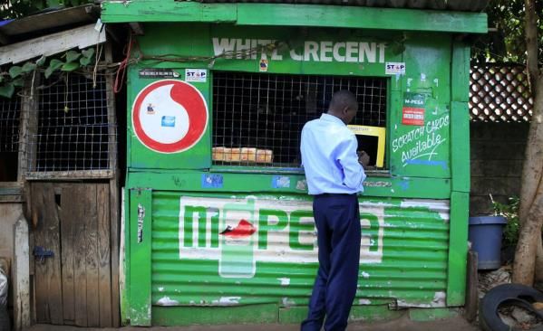
Taking the perspective that small fees are an extremely limiting factor for the poor, M-PESA,
one of the world’s largest mobile money providers has a payment schedule that promotes
account creation for low-income users (Figure 4). Creating an account and balance inquiry are
free to the user, while small day to day transactions have a very low fee. For example, a typical
meal at an inexpensive restaurant would be 400 Ksh ($3.56 USD). To transfer this amount to
another user, the fee would be 6 Ksh ($0.05US), which is about a 1% transaction fee. Where fees
become significant is when a customer wishes to withdraw from an M-PESA agent or ATM.
Withdrawals from a M-PESA agent usually cost twice that of transfer fees, and ATM
withdrawals are even more expensive. This has the potential to discourage customers from
depositing money, knowing that in the future they may need cash for transactions. At the same
Block 4time, high fees for withdrawals, as well as free features, could encourage users to keep their
money within the M-PESA ecosystem. In other words, high switching costs could encourage
individuals to remain within the mobile money ecosystem instead of returning to the cash
economy.
Figure 4: M-PESA Cost Schedule 2021 (Madegwa, 2021)
What is financial inclusion?
The World Bank defines financial inclusion as: “individuals and businesses having access
to useful and affordable financial products and services that meet their needs – transactions,
payments, savings, credit and insurance – delivered in a responsible and sustainable way”
(Understanding Poverty - Financial Inclusion Overview, 2022). Measuring financial inclusion is
based on (1) access; (2) usage; and (3) the quality of financial products and services (G20
Financial Inclusion Indicators – GPFI, 2016). By way of this definition, financial institutions,
governments, and nonprofits must understand the needs and capabilities of financially excluded
populations to have successful policies. Because every individual has different needs and
capabilities, there is no “one size fits all” approach to financial inclusion.
Block 5Adding to financial inclusion, the World Bank defines digital financial inclusion as “the
deployment of the cost-saving digital means to reach currently financially excluded and
underserved populations with a range of formal financial services suited to their needs that are
responsibly delivered at a cost affordable to customers and sustainable for providers” (Kim,
2016). It is possible to be financially included but not digitally financially included. For example,
if an individual only utilizes a traditional bank account. It is also possible that individuals are
only financially included through digital means, such as a family who solely utilizes online
banking to receive direct deposits and pay utilities but does not utilize other services such as
borrowing or savings accounts. In this study, the population includes a nationally representative
sample, capturing individuals of all types of financial inclusion and exclusion. This is useful in
analyzing the potential impact of broad mobile money implementation. For example, it is worth
investigating whether mobile money impacts behaviors of individuals who already have a formal
bank account but may not have digital access to it. For the purposes of this study, individuals
who already have a commercial bank account are included in the sample for this reason.
Mobile money and financial inclusion
To combat poverty, not only must policy makers consider a lack of capital, but they must
also consider the accessibility of tools and resources by which capital can be stored and
transferred. Without these tools, individuals go without protection from financial crises and other
economic shocks. Around the world there are 1.7 billion unbanked adults. Furthermore, a
disproportionate number of unbanked individuals live below the poverty line (Demirguc-Kunt et
al., 2018). Because of this, financial inclusion is the focus of many poverty alleviation initiatives
globally (Chibba, 2009). It has also been found that financial inclusion helps sustain economic
growth within a community (Subbarao, 2009). At the same time, policy makers and researchers
Block 6have identified mobile money as a tool that can be broadly implemented to increase financial
inclusion. It is likely that increasing access to financial services like mobile money is one of the
avenues to reduce poverty, however so far it is unclear what mobile money’s impact is on a large
scale. Therefore, it is important to study mobile money as a tool to boost financial inclusion and
broader economic welfare.
Understanding the potential of mobile money is especially relevant now as the global
adoption of smartphones has lowered barriers for mobile money adoption. Instead of reliance on
physical bank branches, the main requirement for mobile money is to have a cell phone (Hannig
& Jansen, 2010). With immense progress in digital access, this would suggest that mobile money
can be a powerful tool to reach the unbanked.
Block 7Statement of the Problem
The purpose of this research is to test mobile money’s potential as a tool economic
stability and resilience during economic shocks. This thesis analyzes if individuals who utilize
mobile money services show different behaviors in saving, borrowing, and formalized responses
to financial emergencies, relative to those who do not use mobile money. Conducting a meta-
analysis of countries in Africa, Asia, and the Caribbean will begin to reveal general conclusions
about mobile money that can be applied to countries where data is otherwise unavailable, or
where the mobile money networks are emerging.
Block 8Justification of Problem
There are three key reasons that justify research in this area. First, there is a lack of multi-
country analysis. Most methodologies focus on single country analysis. Single country analysis
is common due to challenges of data collection and cleaning across starkly different countries.
Differences between individual national surveys create difficulties with data collection and
aggregation from a variety of country level questionnaires. As a result, it has yet to be
determined whether there are broad, generalizable trends that exist between mobile money and
financial inclusion. Even further, most of these single country analyses are on Kenya, or other
countries where M-PESA has been implemented (Jack & Suri, 2011; Gurbuz Cuneo, 2019;
Ouma et al., 2017; Demombynes & Thegeya, 2012). Understanding mobile money companies
beyond M-PESA will also allow for broader conclusions to be drawn about mobile money.
Second, another substantial portion of the literature has focused on determinants of
individuals adopting mobile money, not specific outcomes such as saving, borrowing, and
economic stability (Amohah et al., 2020; Okello et al., 2018; Honohan and King, 2012).
Understanding specific outcomes is an important next step in this body of literature. Where there
are studies on outcomes, populations tend to be niche and only one outcome is analyzed at a
time. For example, several studies focus on savings behavior of rural farmers, but these
conclusions are not necessarily applicable beyond these specific populations. Understanding
multiple outcomes (saving, borrowing, economic stability) for multiple countries is valuable
when considering future impacts of mobile money where it has not yet been fully implemented.
Finally, the COVID-19 pandemic resulted in adoption of mobile money at a rate
previously unseen. This is due to governments partnering with mobile money companies to
distribute stimulus, as well as the advantages of a digital economy during a public health crisis
Block 9(Appendix 1). Because of this, it is necessary to expand upon understanding of potential outcomes so policymakers can make the best decisions for their countries. Block 10
Theoretical Framework

         The theoretical framework of this paper considers 1.) how financial access and financial

inclusion are measured and 2.) commonly cited barriers to financial access. Both theories are

based on the Global Findex from the World Bank, where survey results and insights come from

thousands of individuals in over 100 countries.

Defining financial resilience

         The theoretical framework of this paper goes beyond the traditional understanding of

financial inclusion. Instead, the framework takes a layered approach to financial inclusion. The

framework begins with financial access, which is the opportunity to take advantage of financial

infrastructure. Financial access answers the question: “what tools are available to meet the

financial needs of a population?” The second layer of the framework is financial inclusion.

Financial inclusion measures whether individuals take advantage of financial access. For

example, the ability to have a debit card is financial access and using a debit card would be

financial inclusion. By this logic, financial inclusion answers the question: “do individuals utilize

financial tools that are available to them?”

         To understand why it is necessary to go beyond financial inclusion, it is important to

consider how financial inclusion is measured and reported. Financial inclusion is measured by

the G20 beginning with financial access, then measuring usage and quality indicators (G20

Financial Inclusion Indicators - GPFI, 2016). “Usage” measures the “regularity” and “duration”

of how financial tools are used (debit card, credit card, cash). For example, does a family

consistently purchase goods with a credit card? Or only when they are short on cash? “Quality”

indicators look to measure if the tools available are appropriate for a specific population.

 Block                                                                                            11
Similarly, if credit cards were available in a community, but very few people qualify for a credit
card, this would not be classified as a quality form of financial inclusion.
Neither usage nor quality indicators attempt to capture long-term changes in behavior
because of financial inclusion. If there is financial access and the tools are utilized and of high
quality, then it is to be expected that financial habits positively change in the long run.
To capture the long-term behavioral impacts of financial inclusion, this framework looks
to add a third layer: financial resilience (Figure 5). Financial resilience answers the question: “to
what extent can individuals withstand economic shocks by using financial tools?” To capture
this, financial resilience measures long-term behaviors such as saving and borrowing habits, as
well as the ability to respond during black swan economic events. Measuring these behaviors is a
way to measure overall improvement in economic welfare and economic stability. For example,
increased saving and borrowing improve overall liquidity, which would improve economic
stability in the event of a family emergency such as illness or death. Improved economic stability
during an economic shock translates to improved economic welfare in the long run.
Figure 5: Levels of Financial Inclusion
Block 12Cited barriers to access
The second part of the theoretical framework that guides this paper is the reported
reasons for being unbanked from the World Bank Global Findex dataset. Globally, one quarter of
respondents surveyed reported costs associated with a bank account, such as fees and time spent
traveling, as reasons for not having a bank account (Demirguc-Kunt et al., 2018). Mobile money
addresses both issues. As mentioned, mobile money eliminates the need to travel to financial
institutions regularly. Additionally, mobile money offers powerful low-cost options. Because
mobile money directly eases commonly cited pain points of financial inclusion, it is worth
testing the impact of mobile money on financial resilience.
Block 13Literature review
First this section outlines the benefits to financial inclusion, as mobile money is regarded
as one of the main tools to reach the unbanked. Then, the second portion of the literature review
serves as the first part of this study’s meta-analysis (Appendix 2).
What are the benefits to financial inclusion?
Several authors suggest that financial access and financial inclusion benefit both
individuals and the countries they live in through poverty reduction, increased human
development, increased economic growth, and lower economic inequality. Because of this, it is
worth studying specific mechanisms by which financial inclusion can increase, such as through
mobile money.
Beginning with financial access, studies consistently show a positive relationship
between increasing financial access and poverty reduction. One of the most notable works in this
body of literature, Finance, Inequality and the Poor, shows that even when controlling for
economic growth, increasing financial access is associated with a drop in the percentage share of
a population that lives on less than $1 a day (Beck et al., 2007). Other studies find that financial
sector growth is associated with poverty reduction (Jaililian and Kirkpatrick, 2005). Financial
sector growth is a form of financial access and would be inclusive of expanding access to mobile
money.
Financial inclusion, like financial access, is associated with poverty reduction. Much
research as suggested that the millennium development goals (MDGs) are not sufficient to
address poverty reduction. However, focusing on financial inclusion related policies is the most
effective way to reach MDGs, such as global poverty reduction (Chibba, 2009). A study on India
suggests that financial infrastructure development and financial inclusion contribute to poverty
Block 14reduction (Williams et al., 2017). A broader study on Asia reports the same results, finding that
financial inclusion has a significant correlation with lower levels of poverty and income
inequality (Park and Mercado, 2018).
Beyond poverty reduction, there are country level benefits to financial inclusion. Strong
correlation exists between financial inclusion and human development within a country (Sarma
and Pais, 2011). Higher levels of human development exist for all, not just those being lifted out
of poverty. Financial inclusion also relates to accelerating economic growth. Research suggests a
chain reaction between financial inclusion, financial development, and country level economic
growth (Mohan, 2006). Regarding financial technology, a recent study claims, “digital financial
inclusion is associated with higher GDP growth” (Sahay et al., 2020). This would suggest that in
the advent of digital technology expansion, inclusive of mobile money diffusion, there is new
opportunity for country-wide growth.
Empirical evidence from other countries
While financial resilience has not been studied directly in a way similar to this thesis,
saving, borrowing, and coping mechanisms have all been studied separately in a variety of
different countries with high mobile money diffusion. These studies serve as the first step to
understanding changes in financial habits and economic stability as a result of mobile money
use.
Saving
Overall, existing literature on individual countries finds that mobile money increases the
likelihood of having savings (Appendix 2). This is consistent across multiple countries and
studies. Less researched has been completed on mobile money’s impact on total saving stock.
However, a number of studies find that savings stock is higher among mobile money users.
Block 15M-PESA, a mobile money company in Kenya, has offered many insights into the impacts
of mobile money. Based on a study of early M-PESA adopters, it is seen that M-PESA is not
only a way to transact, but an informal savings instrument (Jack and Suri, 2011). This paper also
points out that M-PESA users are more likely to use a formal bank account to save than those
without M-PESA, showing that mobile money can serve as a key steppingstone to formal
financial inclusion. Additionally, research suggests that M-PESA increases the likelihood of
having savings but does not examine if total savings stock changes (Demombynes and Thegeya,
2012). Gurbuz Cuneo (2019) confirms and builds on the work of Demombynes and Thegeya
(2012), suggesting that saving among M-PESA users is 16-22 times more likely than among
those without M-PESA. This paper also demonstrates that savings of M-PESA users tend to save
15% of average monthly earnings per household member, but does not compare this to non-users
(Gurbuz Cuneo, 2019).
Moving away from M-PESA, an analysis in Sub-Saharan Africa observes that “not only
does access to mobile financial services boost the likelihood to save, but also has a significant
impact on the amounts saved. These benefits are likely to be the greatest for those with limited
access to the formal banking system” (Ouma et al., 2017). In Rwanda, mobile money
“contributes significantly to savings promotion” when using an endogenous switching regression
model (Maniriho, 2021). However, this paper does not attempt to quantify by how much mobile
money increases savings propensity. Similarly, in a field experiment in India, there are strong
positive perceptions of mobile money, and it is often used as a savings tool for small savers
(Nandhi, 2012). Again, this case study does not attempt to quantify the impact of mobile money.
Evidence from Mozambique is consistent with India and Rwanda where the amount saved
increased in interest bearing mobile money accounts (Batista & Vicente, 2019). In a study done
Block 16in Burkina Faso, likelihood to save is increased by 7-12% when using mobile money when
compared to non-users (Ky et al., 2017). Despite low mobile money penetration in Uganda,
results from Uganda's 2013 FinScope are consistent in that the effect on savings is positive
(Mayanja & Adong, 2016), in addition to this effect on savings in Uganda being confirmed in a
field study (Ryder, 2014). Another study in Uganda suggests that mobile money increases the
likelihood to save by 17% (Munyegera & Matsumoto, 2017). A study conducted on Uganda,
Kenya, and Tanzania indicates that mobile money users are 11% more likely to save compared to
non-account users. This study goes on to explain that mobile money is a compliment to formal
savings, as well as a substitute for informal savings (Ruh, 2017).
The paper Debit Cards Enable the Poor to Save More provides a plausible explanation
for why this occurs. It explains that the difficulty of informal saving is the obligation to find safe
places to store money and the manual, individual accounting a person must do when they do not
have access to a formal account (Bachas et al., 2020). The paper also reports having constant
access to informal savings (stored cash) can decrease total savings as it is easier to spend these
reserves. Finally, in a different paper, Bachas elucidates a correlation between commute distance
to account access and savings stock (Bachas et al., 2018). Broadly, these studies indicated that
lower indirect transaction costs are associated with higher propensity to save.
From these studies in individual countries and niche populations, it is seen that mobile
money has a positive impact on savings. Mobile money can act as an informal savings account, a
steppingstone to formal financial inclusion, as well as lowering indirect transaction costs, which
all lead to increased savings propensity and/or saving stock.
Block 17Borrowing
While it can be debated whether borrowing is a positive or negative outcome, it is seen
that higher financial inclusion and mobile money adoption translate to higher rates of borrowing
(Appendix 2). A study in Asia suggests that higher financial inclusion (broadly defined, not
specific to mobile money) lowers poverty rates, increases entrepreneurship, and increases
borrowing (Park and Mercado, 2021). A study Uganda that also investigated savings propensity
finds that mobile money increases the likelihood of borrowing by 14% (Munyegera &
Matsumoto, 2017). A working paper that analyzes borrowing decisions in a variety of
developing countries has found that individuals who use mobile phones for transactions such as
ecommerce, utilities, and receiving wage payments are 7-17% more likely to borrow (Lyons et
al., 2020). From these studies, mobile money is likely to have a positive impact on borrowing,
which is one of three key components of financial resilience.
Economic shocks and coping mechanisms
Generally, mobile money is positively associated with maintaining consumption during
financial crisis and utilizing formal coping mechanisms during economic shock (Appendix 2). A
study on M-PESA suggests that of households that utilize mobile money, these individuals can
maintain the same level of consumption through negative economic shocks (Jack and Suri,
2014). The study also discovered that households that did not utilize mobile money technology
suffered a 7% decrease in consumption when experiencing a negative economic shock.
Many of the studies that analyzed general savings behavior also analyzed whether
individuals rely on these savings during a financial crisis. In a field experiment in India, many
account users saved specifically for emergencies in an EKO mobile account (Nandhi, 2012).
Similarly, in Burkina Faso it was found that groups that are normally financially excluded, like
Block 18rural populations, less educated groups, and women were able to save for health emergencies
when using mobile money (Ky et al., 2017). Overall, mobile money is associated with increased
ability to cope with economic shocks and maintain economic stability, however the studies
available are limited compared to saving and borrowing.
Rationale for method
There are a variety of methods that have been used to assess the impact of mobile money
due to the lack of natural experiments that can be found in the real world, as well as the lack of
available data (Figure 6). Studies can be grouped into three categories: (1) regression analysis of
large datasets using instrumental variables (2) regression analysis of large datasets without
instrumental variables and (3) smaller sample field studies completed over time (Figure 6).
Often, studies use multiple types of regression models to help explain their results. In general,
different types of regression models and field studies yield the same results: mobile money has a
positive impact on saving and borrowing. However, it is difficult to compare the magnitude of
results across different methods as many countries/populations have only been investigated with
one method. The main difference between these approaches is the level of causality that can be
inferred.
Multivariable regression models are often used because of their simplicity to implement.
These models are a great start for beginning to identify relationships between variables of
interest. However, it is difficult for standard multivariable regression models to be considered
causal, even with many controls. Instrumental variable regression models share many similarities
with multivariable regression models but are more difficult to implement. At times, instruments
may be unavailable, weak, or theoretically flawed. Causal results can come from instrumental
variable regression, but this is contingent on the strength of the instrument. Finally, field studies
Block 19require lots of time, effort, and capital to implement. In terms of small sample sizes, it is possible
to have controls that lead to casual results. However, it is difficult to do a field experiment on a
sample size large enough to answer the questions of this study.
Studies vary slightly in the variables analyzed, depending on the availability of data and
survey respondents. Typically, financial inclusion is a function of demographic characteristics
and income related measures. Studies that use instruments to improve their regression typically
use the same instrument, which relates to distance away from a financial access point, like a
mobile money agent.
Figure 6: Methods Used by Existing Studies
Regression, no instrument Maniriho (2021); Ouma, Odongo, Were (2017)
Regression, instrument Ky et al. (2017); Mayanja & Adong (2016); Ruh (2017);
Demombynes and Thegeya (2012); Gurbuz (2017); Honohan,
P., & King, M. (2012)
Field study Nandhi (2012); Batista & Vicente (2019); Ryder (2014); Jack
and Suri (2011); Jack and Suri (2014)
This study will utilize OLS regression and IV regression is ways similar to prior studies.
Additionally, this study will attempt to use the same types of variables utilized in past studies.
The main difference, however, is that this study will analyze many countries at once and solely
focus on the mobile money coefficient as it impacts saving and borrowing propensity. As coping
mechanisms are often analyzed using field studies, this study will complete descriptive analysis
to identify if there are similar conclusions.
Block 20Methodology
This study uses available data from FinScope surveys collected from nine countries with
a total size of 60,375 individuals (FinMark Trust, 2015). The countries analyzed are Benin,
Burkina Faso, Cameroon, Eswatini, Haiti, Madagascar, Rwanda, Togo, and Zambia. The data
collection of these surveys ranges from 2015-2019. This is acceptable, as it reflects the impacts
of mobile money broadly, no matter the stage of mobile money diffusion into a country.
Specifically, each country only has data from one period. From the FinScope survey, data from
18 survey questions was used to create variables of interest (Appendix 3). Summary statistics for
variables used are in the table below.
Figure 7: Summary Statistics
Variable Description Variable Name Observations Mean StDev
Country Country 67345
Mobile money use (y/n) MM 67345 0.24 0.43
Distance from Mobile Money Agent DistMM 42925 50.38 44.44
Commericial Bank Account Use (y/n) CB 67345 0.13 0.33
Distance from Commercial Bank Account DistCB 34118 58.96 43.52
Urban / Rural UrbRur 67345
Age Age 58847 38.65 16.12
Education Level Education 56482 3.07 1.56
Head of Household (y/n) HoH 67345 0.59 0.49
Personal Income (Numeric) PersonalInc 33767 173066.08 1818905.30
Personal Income (Percent Rank) PI_Perc 33767 0.55 *+
Household Income (Numeric) HHInc 29903 291995.81 2130953.94
Household Income (Percent Rank) HI_Perc 29903 0.58 *+
Combined Household and Personal Income (Percent Rank) IncPerc 39368 0.56 *+
Total Savings Reported (Numeric) SaveNum 17092 1145849.01 6723271.22
Total Savings Reported (Percent Rank) SN_Perc 17092 0.48 *+
Indicated Savings (y/n) SaveBin 67345 0.56 0.50
Total Debt/Borrowing Reported (Numeric) BorrowNum 11886 1601087.78 13283345.76
Total Debt/Borrowing Reported (Percent Rank) BN_Perc 11886 0.48 *+
Indicated Borrowing (y/n) BorrowBin 67345 0.31 0.46
*Mean is not exactly .5 because this is a discrete variable, not continous, so multiple reported values may have the same rank
+ Uniform
Models
For each outcome, saving and borrowing, there are 5 models (Figure 8). Three of the
models are instrumental variable regressions utilizing different combinations of variables. Two
of the models are ordinary least squares models, each also utilizing different combinations of
variables. The OLS acts as a first step to understanding the relationship between mobile money
Block 21and financial resilience, while using an IV regression estimates the causal impact of mobile
money on financial resilience.
The creation of the OLS(2) model was based on other studies like this one, where all
proposed variables are put into one model. For purposes of better understanding the impact of the
control variables, a simple OLS(1) regression model was created, with only one explanatory
variable, mobile money use. A low VIF, as well as the use of both financial access and
demographic variables in the same model in other studies, did not suggest potential endogeneity
issues. Theoretically, there may be an endogeneity issue, but the OLS models in this study serve
the purpose of testing my results against previous studies that used similar methods.
For the IV regression model, however, a high VIF indicated that there may be an
endogeneity problem when using all proposed variables in the same model in addition to the
instrumental variable. To overcome this, the IV models group variables between demographic
variables (Urban/Rural, Age, Education, Head of Household) and financial access variables
(income, commercial bank account use). For example, income may be a function of age and
education level, so these predictor variables should not be utilized in the same model. Splitting
the models between demographic and financial access variables resolved the VIF issue and is
logically sound to solve the endogeneity problem. Like the OLS model, a basic IV model using
only mobile money as the explanatory variable is used to compare the impacts of different
variable groupings (demographic variables compared to financial access variables). The 5
general models for each outcome variable are described below.
Block 22Figure 8: General Model Description
Without controling for demographic variables or differences in financial access, what is
COUNTRY_ IVREG: the impact of mobile money on the likelihood to save, using distance from a MM agent
as an instrument
Controling for demographic variables, what is the impact of mobile money on the
COUNTRY2_IVREG:
likelihood to save, using distance from a MM agent as an instrument
Controling for financial access, what is the impact of mobile money on the likelihood to
COUNTRY3_IVREG:
save, using distance from a MM agent as an instrument
Without controling for demographic variables or differences in financial access, what is
COUNTRY_OLS:
the impact of mobile money on the likelihood to save
Controling for demographic and financial access variables, what is the impact of mobile
COUNTRY2_OLS:
money on likelihood to save
Analysis of savings propensity and borrowing propensity is the first step in telling a
complete story of mobile money’s impact on financial resilience. Each model was then applied
to savings propensity and borrowing propensity for each country (Figure 9).
Figure 9: Detailed Model Description
SaveBin
COUNTRY_IVREG SaveBin ~ MM | DistMM
COUNTRY2_IVREG SaveBin ~ MM + UrbRur + Age + Education + HoH | DistMM
COUNTRY3_IVREG SaveBin ~ MM + IncPerc + CB | DistMM
COUNTRY_OLS SaveBin ~ MM
COUNTRY2_OLS SaveBin ~ MM + UrbRur + Age + Education + HoH + IncPerc + CB
BorrowBin
COUNTRY_IVREG BorrowBin ~ MM | DistMM
COUNTRY2_IVREG BorrowBin ~ MM + UrbRur + Age + Education + HoH | DistMM
COUNTRY3_IVREG BorrowBin ~ MM + IncPerc + CB | DistMM
COUNTRY_OLS BorrowBin ~ MM
COUNTRY2_OLS BorrowBin ~ MM + UrbRur + Age + Education + HoH + IncPerc + CB
Block 23Instrument rationale
The need for an instrumental variable comes from a large potential for influence from
confounding variables on the relationship between mobile money adoption and financial
resilience. For example, an individual who knows of mobile money might also recognize the
benefits to saving and borrowing. Similarly, an individual may not save or use mobile money
platforms for the same reason: lack of money, lack of trust, or lack of financial education
(Demirguc-Kunt, 2018). Because of this, an instrument is needed to assess the causal relationship
between mobile money and financial resilience.
The instrument for the IV models is the reported time to travel to a mobile money agent.
For example, in the FinScope survey, an individual can report that it takes them 5 minutes to get
to a mobile money agent. Other studies previously mentioned use geographic distance as an
instrument. Many studies utilize geospatial data available for mobile money locations in Kenya
as it relates to the M-PESA program to create an instrumental variable. However, accurate
geospatial data is not available for all the countries in this study, so distance reported as time is
used as a proxy.
This is an acceptable instrument because distance from a mobile money agent should not
correlated with financial resilience (propensity to save, borrow, and coping mechanisms) but
should be correlated with the propensity to adopt mobile money.
First, any existing predisposition to save as a result of culture, upbringing, and
psychological factors is not impacted by the existence of mobile money locations. It could be
assumed that mobile money agents exist in communities where individuals are of higher
economic status, and therefore they save more based on their wealth and disposable income.
However, mobile money agents serve financially excluded individuals. Typically, financially
Block 24excluded individuals are of lower economic status. This factor suggests that financial resilience
(as it relates to savings) should not be positively correlated with the distance away from a mobile
money agent.
However, a meaningful negative correlation would also not satisfy the requirements to be
a valid instrument. Something unique to mobile money agents is that deposit and withdrawal
locations are in shops, markets, convenience stores, and other common locations. The locations
are more likely to be randomly and evenly distributed as compared to bank branches, limiting the
potential for a meaningful negative correlation.
Additionally, the likelihood of a meaningful negative correlation is mitigated by the fact
that mobile money is not advertised as a savings tool. Mobile money agents will likely be located
where individuals seek to do transactions with or without formal means, like credit cards. So, this
can eliminate some elements of self-selection as all individuals need to transact, further
justifying the random relationship between distance from a mobile money agent (Z) and
propensity to save (Y).
When considering whether borrowing behavior is associated with distance away from a
mobile money agent, it is important to remember that traditional banks can be lenders, while
mobile money agents are not. It is very possible that an individual uses mobile money for day-to-
day needs, then chooses to apply for a loan from a friend, family member, microlender, or a
traditional bank. These are common sources of loans in many countries where the traditional
banking sector does not reach all individuals. Given the diverse options available for a loan, it is
not likely that the location of mobile money agents is correlated with the likelihood of applying
for/receiving a loan.
Block 25Finally, this study does not propose an instrumental variable regression to predict coping
mechanisms during a financial crisis, so these relationships are not relevant. However, this study
looks to find a consistent story between regression outputs for saving and borrowing and the use
of different coping mechanisms. Logically, individuals who have more savings and the ability to
borrow quickly and reliably are more likely to withstand economic shocks without severe harm.
Based on this rationale, it follows that distance (in time) away from a mobile money
agent should be a sufficient instrument for my analysis when considering the attributes of mobile
money theoretically. However, the instrument must also be statistically and mathematically
sound. To be a sufficient instrument, the correlation between mobile money use (X) and distance
away from a mobile money agent (Z) must be strong. The correlation between X and Z for the 9
countries ranges from -.3 to -.45. That is, the further away an individual is from a mobile money
agent, the less likely they are to use mobile money with a correlation of .3-.45. While many
instruments ideally have a correlation > .6, the range of .3-.45 is sufficient considering that
mobile money use (X) is binary and that reported distance from mobile money agent (Z) is
discreet1. Should these variables be continuous, for example mobile money usage frequency or
exact distance from mobile money agent, this correlation would likely be higher. That is, the
instrument is theoretically sound, but could be stronger. The model outputs are strengthened by
other control variables, nonetheless.
Additionally, to be a sufficient instrument, the correlation between Y (saving propensity,
borrowing propensity) and Z (distance in time away from a mobile money agent) must be
negligible. Where sample size of mobile money users is sufficient (Appendix 4)2, the correlation
1
For the FinScope surveys, distance away from a mobile money agent could be reported in increments of 5, 10, 15,
20, 30, 45, and 60 minutes.
2
In the original dataset for this study there was 67,345 observations from 11 countries. This paper included Gambia
and Myanmar for all parts of the analysis, until it was realized that the use the instrument, distance from a mobile
Block 26of Y and Z ranges from .009 to -.07, which is low enough to confirm no significant relationship
between Y and Z, further demonstrating that the instrument of choice is valid. This is consistent
with the hypothesis above regarding low income and financially excluded communities, as well
as the more randomized placement of mobile money agents as to bank branches.
Descriptive analysis
Due to the nature of the survey data being at times incomplete, especially in questions
that require manual entry or questions towards the end of the survey, regression analysis is not
appropriate to analyze numeric saving or numeric borrowing variables. Additionally, descriptive
analysis is used to identify trends in coping mechanisms. The goal of these analyses is to help
support the findings of the IV and OLS regressions and to help create a story that surrounds the
outputs. Descriptive analysis of these variables serves as a robustness check for the 5 models
created.
money agent, was statistically weak in these countries. This best explained by the fact that both countries have very
low rates of mobile money diffusion and adoption, over-emphasizing variation within the small sample proportion
of mobile money users. The weak instrument resulted in consistently insignificant results with outlier coefficients.
However, there results were likely due to the low sample proportion of mobile money users and not representing the
impact of mobile money on individuals within these countries.
Block 27Assumptions and Limitations
This methodology has 3 key assumptions: 1.) The instrumental variable is strong and
appropriate 2.) FinScope surveys are nationally representative 3.) The variety of countries with
data available (in addition to other studies) is sufficient to draw broad conclusions about mobile
money.
Based on the explanation and assumptions above, the proposed instrument of mobile
money agent concentration is appropriate. That is, saving and borrowing are only impacted by
distance away from a mobile money agent through its relationship with mobile money adoption.
Beyond the previous explanation and assumptions, the use of a geographic instrument (distance
reported in travel time) is well documented in developmental economics and healthcare
economics, providing further justification for its use. This instrument could be made stronger by
using continuous variables, as the instrumental variable used was captured in the survey as a
discrete variable.
When using the FinScope data, this study does not seek to confirm whether FinScope
data are truly nationally representative. Given that the agencies that collect this data, as well as
other studies that rely on the same data, report that the data is nationally representative this is a
strong assumption in the analysis. However, with in-person surveys of this size, as well as
potential changes in demographics over time, there is a risk that these data sources may not be
nationally representative. Should the data not be nationally representative, or should the national
makeup of a country strongly vary between the date of collection and present day, this would
create limitations and potential estimation error in reported findings.
Finally, there may be features of the countries analyzed in this study, as well as the other
individual studies, which allow mobile money to create a positive impact on financial resilience
Block 28that are rare / not present in other countries in the world. This study attempts to analyze a variety
of countries in different parts of the world, but many of these countries are studied because of the
existence of mobile money. Further, mobile money exists in these countries because individuals
are financially excluded. Therefore, these results may be attributable to financial inclusion alone
(mobile money as the only option). This means that mobile money may have less impact where
traditional banking already exists.
Building further on this, the results from the descriptive analysis in the third part of this
thesis are not causal, so concrete conclusions cannot be drawn until they are tested with more
rigorous statistical methods. The direction of the results (positive or negative) helps further
understand what is occurring with mobile money in these countries, however these results should
not be overapplied when attempting to come to broad conclusions about mobile money.
There are many obstacles and deficiencies in the current literature that call for a study
like this. However, these same obstacles and deficiencies can also limit the accuracy and
applicability of prior studies that serve as the basis for this study. As a result, more field studies
or additional surveys are needed in order to confirm the repeated findings of the FinScope data.
Block 29Results
Across all countries, the IV regression models suggest mobile money increases
propensity to save by 21% on average (Appendices 5-7). Propensity to borrow also increases by
10% on average across all IV models when mobile money is used (Appendices 8-10). Both
outcomes are consistent with previous studies of other countries. Using descriptive methods,
results also suggest a positive relationship between total savings stock and mobile money use, as
well as a positive relationship between total amount borrowed and mobile money use. These
findings support the analysis of coping mechanisms, where mobile money users are more likely
to use formal coping mechanisms during economic crises, and less likely to use informal coping
mechanisms.
The use of instrumental variable regression to analyze savings propensity and borrowing
propensity yields a wider range of results than the OLS regression, as well as larger confidence
intervals. This is to be expected, as the instrument attempts to eliminate psychological and
environmental influence that would simultaneously reinforce both financial resilience (saving
and borrowing) and mobile money use.
Saving propensity
Overall, models suggest that mobile money use is associated with a higher propensity to
save. The preferred OLS and IV models suggest the range of 11%-30% increase in savings
propensity due to mobile money use, which is consistent with prior studies.
The OLS(1)-Saving regression model indicates that across countries, on average the
propensity to save is 20% higher for mobile money users when not controlling for other factors.
Significant coefficients for propensity to save range from 35% to 8% (Figure 10). This model
serves as a base to compare OLS(2)-Saving, and these results should not be interpreted as the
Block 30true impact of mobile money on savings propensity. Adding in demographic and financial access
control variables, the effect of mobile money is estimated to be smaller. The OLS(2)-Saving
regression model suggests that on average, saving is 11% higher for mobile money users, with
country-specific estimates ranging from 22% to -.03% for all coefficients, demonstrating the
impact of the demographic and financial access control variables decreasing the mobile money
coefficient in the model relative to OLS(1)-Saving (Figure 10). The smallest coefficient, .03% in
Madagascar, is result was not statistically significant in the OLS(2)-Saving regression, but all
other observations in OLS(1)-Savings and OLS(2)-Savings are significant. Both OLS models,
while not causal, suggest a positive relationship between mobile money and savings propensity.
Figure 10: OLS Savings Models
Appendix 11 and Appendix 12 offer exact results in tabular form
Turning to the IV models, which help in moving beyond correlation to identify causal
effects, the IV(1)-Saving regression model indicates that propensity to save increases by 33% for
mobile money users (Figure 11). The largest increase was 77% and the smallest increase was
Block 3110%. This regression has no controls, and is used to compare the effects of demographic
variables in IV(2)-Saving and financial access variables in IV(3)-Saving.
Adding demographic controls, the IV(2)-Saving regression model suggests that mobile
money increases propensity to save by 30% on average. Contrastingly, the IV(3)-Saving
regression model shows that mobile money increases propensity to save by 12% on average,
when including financial access control variables (Figure 11). Nonetheless, between the two
models, the majority of countries fall between 10-30% increases in savings propensity for mobile
money users.
Figure 11: IV Savings Models
Appendix 5, Appendix 6, and Appendix 7 offer exact results in tabular form
When comparing the OLS and IV models, it is seen that IV(3)-Savings (financial access
controls) and OLS(2) have the most similar coefficients. At the same time IV(2)-Savings
(demographic controls) suggests a much higher result (Figure 12). This could suggest that the
combination of financial access controls and the instrument is the most appropriate for
Block 32explaining the variation in savings behavior that is caused by mobile money. Alternatively, differences in the IV(2)-Savings regression (demographic controls) could be explained by the “local average treatment effect” (LATE). This is where the IV coefficient results reflect the impact on savings for those affected by the instrument, distance from a mobile money agent. At the same time, it would not reflect the impact on savings for those not affected by the instrument (Becker, 2016). So, it could be that those who live very close to a mobile money agent have a higher propensity to save than those who live far away from a mobile money agent. It’s very possible that those who report low times to mobile money have private transportation, which could also translate to a higher propensity to save relative to those who rely on public transportation and/or walking. In the case of IV(3)-Savings, financial access controls may do a sufficiently better job at capturing the impact on savings for the entire sample, decreasing the effects of LATE. That is, financial access variables, when combined with the mobile money predictor and instrument, best capture the behavior of the entire population as income and commercial bank account ownership may capture unidentifiable confounders in a similar way to the instrument, or at least better than the demographic controls in IV(2)-Savings (demographic controls). Alternatively, it’s possible that there is an endogeneity problem with the OLS(2)- Savings model. Although this study chose to mimic the variable selection of past studies, there is likely endogeneity between the financial access and demographic variables that were both included in the OLS(2)-Savings model. Block 33
Figure 12: Comparing OLS and IV Savings Models

Borrowing propensity

         When compared to the savings models, the results on borrowing are more mixed. While

coefficients are generally positive, there are several more instances of insignificant results when

compared to the Savings models. Relevant IV models suggest mobile money increases

propensity to borrow by 7-13% on average.

         The OLS(1)-Borrow regression model indicates that propensity to borrow is 10% higher

for mobile money users without any controls (Figure 13). Individual country results range from

14% to 6%. All countries in the OLS(1)-Borrow model are significant, however this model is not

reliable due to only predictor variable, mobile money use, being used in the model. This model

serves as a baseline to compare OLS(2)-Borrowing. When applying controls, the OLS(2)-

Borrow regression model indicates that propensity to borrow is higher 8% for mobile money

users. The coefficients range from 11% to 4%. Again, all models are statistically significant, and

 Block                                                                                           34
You can also read