Minimizing form errors in additive manufacturing with part build orientation: An optimization method for continuous solution spaces - De ...
←
→
Page content transcription
If your browser does not render page correctly, please read the page content below
Open Engineering 2022; 12: 227–244
Regular Article
Torbjørn L. Leirmo* and Oleksandr Semeniuta
Minimizing form errors in additive manufacturing
with part build orientation: An optimization
method for continuous solution spaces
https://doi.org/10.1515/eng-2022-0032 PCS part coordinate system
received August 27, 2021; accepted January 04, 2022 STL STereoLithography file format
Abstract: For additive manufacturing (AM) to be success- VE volumetric error
fully implemented in manufacturing systems, the geo- WCS world coordinate system
metric accuracy of components must be controlled in
terms of form, fit, and function. Because the accuracy
of AM products is greatly affected by the part build orien- 1 Introduction
tation, this factor dictates the achievable tolerances and
thereby the ability to incorporate AM technologies in a Additive manufacturing (AM) holds the potential to revo-
large-scale production. This article describes a novel lutionize the manufacturing industry through topology-
optimization method for minimizing form errors based optimized lightweight structures and mass-customized
on the geometric features of the part. The described designs. However, the full potential of the technology
method enables the combination of separate expressions remains largely unexploited due to cost restrictions and
for each feature to create a continuous solution space. quality issues. While AM is utilized in medical, aero-
Consequently, the optimal part build orientation can be space, and automotive industries for small production
precisely determined based on a mathematical descrip- volumes, this is only possible because every component
tion of the effect of build direction on each surface type. is carefully engineered and validated through an iterative
The proposed method is demonstrated in two case stu- process before production is initiated. For mass customi-
dies by step-by-step descriptions including discussions zation to truly reach its potential in agile manufacturing,
on viability and possible extensions. The results indicate automated process planning for AM must be developed to
good performance and enable flexible prioritization and ensure quality and consistency in the production.
trade-offs between tolerance characteristics. While AM offers design freedom to create innovative
free form surfaces previously unattainable by conventional
Keywords: additive manufacturing, part build orienta- manufacturing methods, traditional shape features will still
tion, quality, accuracy, build direction, optimization be present in novel designs, such as the interfaces between
components of an assembly. The interconnection between
Abbreviations AM and conventional manufacturing technologies in man-
ufacturing systems warrants the control of geometric accu-
AM additive manufacturing racy in terms of traditional tolerancing features.
EA evolutionary algorithm To enable consistent production of unique compo-
FFF fused filament fabrication nents while meeting quality requirements, it is necessary
GA genetic algorithm to develop valid models and methods for predicting, miti-
gating, and adapting to variation in the build process.
One of the major determining factors for geometric accu-
* Corresponding author: Torbjørn L. Leirmo, Department of racy in AM is the part build orientation, i.e., the direction
Manufacturing and Civil Engineering, Faculty of Engineering, NTNU - in which the material is added to the substrate to realize
Norwegian University of Science and Technology, Gjøvik, Norway,
the geometry [1]. This article describes a method for the
e-mail: torbjorn.leirmo@ntnu.no
Oleksandr Semeniuta: Department of Manufacturing and Civil
precise determination of optimal part build orientation to
Engineering, Faculty of Engineering, NTNU - Norwegian University of minimize the deviations from nominal to the actual geo-
Science and Technology, Gjøvik, Norway metry by considering the geometric features of the part.
Open Access. © 2022 Torbjørn L. Leirmo and Oleksandr Semeniuta, published by De Gruyter. This work is licensed under the Creative
Commons Attribution 4.0 International License.
228 Torbjørn L. Leirmo and Oleksandr Semeniuta
The accuracy of an additively manufactured surface
partly depends on its curvature (or lack thereof). Therefore,
the proposed method enables separate mathematical models
to be applied to each surface type. These models are then
populated with data from the CAD model and combined into
a single expression of quality as a function of part build
orientation. The result is a continuous objective function
for the entire solution space, which enables the identifica-
tion of optimal part build orientations or feasible regions for
Figure 1: Illustration of the staircase effect and the cusp height
secondary objectives.
introduced by layered manufacturing.
The remainder of this article is structured as follows:
First, the theoretic foundations and previous work are
calculated from the layer thickness hlayer and surface
outlined in Section 2 before the method is described in
angle θ , which is the angle between the build direction
Section 3. In Section 4, two case studies are presented to →
demonstrate the method step by step before a brief dis- ẑ = [0 0 1] and the surface normal vector n as described
cussion on the viability and possible extensions is pre- by Alexander et al. [5]:
sented in Section 5. Finally, Section 6 summarizes this hlayer∣cos θ∣ , if ∣cos θ∣ ≠ 1,
article and provides directions for the future work. hcusp = ⎧ (1)
⎨
⎩ 0, if ∣cos θ∣ = 1.
Another measure of the staircase effect is the volu-
metric error (VE) introduced by Masood et al. [6], which
2 Theoretic background corresponds to the volumetric difference between the
CAD model and the realized geometry. This solution
In general, AM techniques successively add layers of soon becomes quite complex when extended from two
material to create an object [1]. This layered manner of to three dimensions. Figure 1 illustrates the deviations
fabrication is a decisive factor in how accuracy errors due to the staircase effect where the area below the
occur in the AM process. Dantan et al. [2] identified a dashed line is lost. The VE is the result of integrating
range of defect modes in fused filament fabrication, this area along the perimeter of the layer. Complex sur-
many of which can be extended to other AM technologies. faces drastically complicate the computation of VE, and
Defect modes relating to the direction of material deposi- simplifications are often necessary.
tion, as well as errors in the machine/tool movement, The obvious solution for mitigating the staircase
influence the accuracy of the produced surface regardless effect is to make sure all surfaces are oriented either par-
of technology and material. Apart from the various sur- allel or perpendicular to the build direction. However,
face defects and inaccuracies present in most AM pro- when a part consists of several features in different direc-
cesses, the products also exhibit anisotropic mechanical tions (which is the case for most functional components),
properties where the behavior depends on the build there will be no part build orientation in which all sur-
direction [3]. Consequently, the part build orientation is faces are either parallel or perpendicular to the build
a decisive factor in the final part quality in terms of both direction. Furthermore, curved surfaces do not benefit
accuracy and mechanical properties. from perpendicular orientations as this will maximize
The staircase effect is perhaps the most illustrative the staircase effect. Therefore, a trade-off must be made
example of how part build orientation is vital in AM. to converge on a globally optimal solution, where the
The layered manufacturing approach inevitably leaves a staircase effect is minimized. The orientation problem
characteristic pattern on inclined surfaces. This pattern for accuracy is however composed of many more failure
emerges when the contours of two subsequent layers modes other than the staircase effect, all of which matters
cannot align perfectly. The result is a stepped surface in modeling the final geometry.
as displayed in Figure 1, commonly referred to as the While the part build orientation should be consid-
staircase effect. ered in the design stage, this is not always possible.
The staircase effect can be modeled in two dimen- Consequently, the information available when deciding
sions as the cusp height hcusp , i.e., the shortest distance the part build orientation may differ from full CAD model
from the inner corner of a step, to the hypotenuse of the with tolerances, to the tessellated STereoLithography file
right triangle of Figure 1 [4]. The cusp height may be format (STL) commonly used in the final stages of process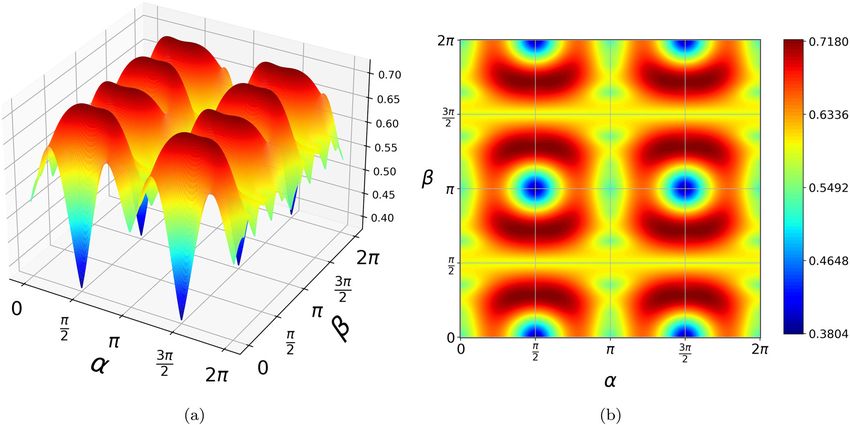
Minimizing form errors in additive manufacturing with part build orientation 229
planning for AM. Naturally, methods for dealing with the hull) or by discretization of the solution space, i.e., cer-
orientation problem with these varying knowledge levels tain intervals of rotation about one or more predefined
have been proposed in the literature – some relying on axes. In the next step, either an exhaustive search is
computational methods and others on a human expert. In performed where all candidates are considered or a guided
addition, some may focus on finding a minimal solution search is conducted, e.g., by a genetic algorithm (GA).
fast, while others may prefer to spend more time to find These discrete methods have certain advantages, but
the optimal orientation. The many possible combinations they inherently fail to consider the entire (continuous)
of methods, objectives, and limitations have resulted in a solution space and therefore risk missing good orienta-
plethora of approaches ranging from the general to the tions. In addition, any attempt to refine the search space
highly specific. However, the crux of the orientation pro- by including more candidate orientations inevitably
blem remains to achieve the best possible result with the increases the computation time.
information at hand, within a reasonable time. The second group, on the other hand, grants access
to the entire solution space, where the complexity of this
solution space generally correlates with the complexity of
2.1 Related work the geometry. This category is not as well explored, per-
haps due to the simplicity of discrete solution spaces or
Part build orientation is a key factor in AM as it is easily the ability of discrete approaches to handle discontin-
manipulated and has a clear influence on final properties. uous functions. Nevertheless, a continuous solution space
The effect of part build orientation has been the subject of may facilitate more nuanced objective functions and com-
many research efforts but remains an open issue [7]. plex solution spaces. Continuous solution spaces can be
Methods for determining the optimal part build orienta- explored by evolutionary algorithms (EAs), or gradient-
tion can be largely divided into two groups: (i) those based methods where knowledge of the topology of the
evaluating a set of candidate solutions with respect to solution space is exploited in an iterative search for the
an objective function and (ii) those mathematically describing global optimum.
the solution space to explore this continuous space for the The approach described herein constitutes a hybrid
optimal solution. A selection of the most relevant related of the two methods outlined earlier: The solution space is
methods is showcased in Table 1. The interested reader described with a differentiable function, which is used to
may refer to refs [7,8] for recent reviews on the orientation identify critical points. The critical points will then con-
problem. stitute the candidate orientations in the final evaluation,
The first group is the most common and starts by which identifies the global optimum. The novelty of this
identifying candidate orientations. This process is either approach lies in the combination of simplicity from gen-
based on a set of rules (e.g., flat surfaces of the convex eralizing surface types, and the flexibility brought
Table 1: Characteristics of related work in chronological order
Reference Candidate orientations Search method
Cheng et al. [9] Flat surfaces ES
Alexander et al. [5] Flat surfaces + user defined ES
Masood et al. [10] Discretized solution space ES
Byun and Lee [11] Faces of convex hull ES
Padhye and Deb [12] All EAs
Zhang and Li [13] Discretized unit sphere ES and EA
Li and Zhang [14] Discretized unit sphere EA
Das et al. [15] All GBM
Zhang et al. [16] Discretized unit sphere ES
Das et al. [17] All GBM
Budinoff and McMains [18] Discretized unit sphere ES
Chowdhury et al. [19] All GBM
Zhang et al. [20] Facet clusters ES
Qin et al. [21] Facet clusters ES
ES = exhaustive search, EA = evolutionary algorithm, GBM = gradient-based method.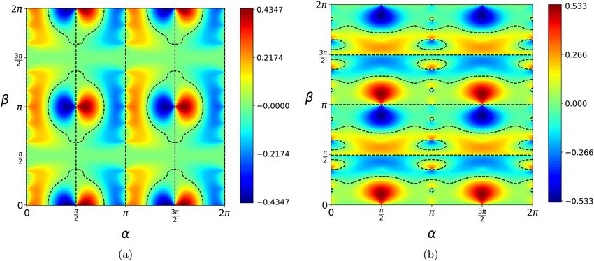
230 Torbjørn L. Leirmo and Oleksandr Semeniuta
forward by the general framework that can be populated The existing body of literature describes various
with any objective function. approaches to the orientation problem with various bene-
Cheng et al. [9] considered all flat surfaces as candidates fits and drawbacks. Exploiting higher level information
for determining the optimal part build orientation and eval- about local topology facilitates the generation of candidate
uated every candidate orientation with respect to the accu- orientations. This information can also be used to con-
racy, build time, and stability. A similar approach was struct continuous solution spaces for achievable toler-
proposed for the minimization of cost by Alexander et al. ances and other objectives. The method presented herein
[5] who included the cost of postprocessing and build benefits from the generalization of part geometry to reduce
time in the cost calculations. Zhang et al. [16] generated the number of parameters in optimization, while also acces-
a set of candidate orientations from every shape feature sing the entire solution space for mathematical analysis.
and evaluated them for several attributes including sur-
face roughness and support volume. Similar methods
have also been proposed with facet clustering, where
2.2 Mathematical foundations
groups of facets are considered collectively based on how
they are affected by part build orientation [20–21]. All these
There is no shortage of mathematical formulations of
methods benefit from the generalization of how different
the orientation problem in the academic literature. The
surfaces are affected by the build direction. While various
plethora of formulations arises from the subtle differences
methods are employed in these studies in the search for an
in AM technologies, which have varying parameters with
optimal solution, none of them consider a continuous solu-
different effects. The number of formulations is further
tion space generated from the geometry.
amplified by the deviating scope and objectives of pre-
Zhang and Li [13] proposed a discretization of the
vious works. For instance, the VE is a common measure
solution space (i.e., a unit sphere), and let each facet of
of accuracy in AM. However, the calculation of VE is based
the STL file promote the two orientations parallel to the
on fundamental assumptions regarding the surface profile,
facet normal, as well as the great circle corresponding to
typically assuming right-angled steps. However, the real
the perpendicular of the normal vector. The authors
surface will be filleted as various effects will round off the
describe methods to make the selection using an exhaus-
corners and hence throw off the theoretical models [26,27].
tive search for minimizing VE, as well as a GA for com-
Nevertheless, the effect of part build orientation on
bined optimization of VE and part height [13,14]. The
surface accuracy is indisputable in the current AM sys-
authors argue for the use of GA over exhaustive search
tems, although of less concern when the layers are thinner
when the number of discretized points becomes large due
[28]. Therefore, the modeling of quality as a function of
to time concerns. Discretization allows for controlling
part build orientation is warranted, and mathematical
the resolution of the solution space and therefore also
descriptions of orientations are necessary.
the computational cost. However, the approach remains
According to Euler’s rotation theorem, any orienta-
oblivious to any effects other than those of the predefined
tion of a rigid body in 3 can be described as a sequence
points in the solution space.
of three basic rotations (α, β , γ ), where no two subse-
Das et al. [15,17] proposed a method for minimizing
quent rotations are performed about the same axis. The
form errors and support structures by formulating a
basic rotations are performed about the x -, y -, and z -axis
minimization problem to be solved in MATLAB with gra-
individually, and a rotation of θ degrees about the respec-
dient-based optimization. The method is based on the one-
tive axes can be calculated using the 3 × 3 rotation
dimensional tolerance maps of Paul and Anand [23,24] for
matrices Rx , Ry , and Rz where
cylindricity and Arni and Gupta [25] for flatness – both
theoretically derived from the staircase effect. A similar ⎡1 0 0 ⎤
approach was proposed by Chowdhury et al. [19] who Rx (θ ) = ⎢ 0 cos θ − sin θ ⎥ , (2)
⎢
⎣ 0 sin θ cos θ ⎥ ⎦
continued to compensate the geometry for any expected
deviations still present after optimization. However, both
⎡ cos θ 0 sin θ ⎤
of these proposed methods involve a risk of convergence Ry (θ ) = ⎢ 0 1 0 ⎥, (3)
to local optima due to the gradient-based approach. The ⎢
⎣ − sin θ 0 cos θ⎥
⎦
convergence to local optima is avoided in the study by
Budinoff and McMains [18] who performs an exhaustive ⎡ cos θ − sin θ 0 ⎤
Rz (θ ) = ⎢ sin θ cos θ 0 ⎥ . (4)
search of one-degree increments to identify feasible regions ⎢ 1⎥
⎣ 0 0 ⎦
from which the final orientation may be selected.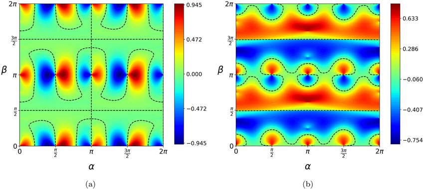
Minimizing form errors in additive manufacturing with part build orientation 231
The rotation matrices of equations (2)–(4) will rotate schemes. In this context, a shape feature is defined as
any column vector about the respective axis by the angle θ . either a geometric primitive, i.e., plane, cylinder, cone,
The direction of the rotation is determined by the right- sphere, or torus (Figure 2), or a free-form surface. These
hand rule, i.e., counterclockwise as seen from the positive feature types are affected by the build direction in different
end toward the origin. According to Euler, any orientation ways and are also subject to different tolerance character-
can be achieved by three successive rotations. However, istics such as flatness, cylindricity, etc. Therefore, these
because matrix multiplication is non-commutative, the features should be used in the construction of the objective
sequence of rotations influences the final orientation of function.
the body. Consequently, when three rotations are per- The current method requires information about the
formed in succession following Euler’s rules, there are still feature types and the relative orientation of the features.
12 possible combinations divided into two distinct groups: This information is readily available in many 3D-file
(1) Proper Euler angles where the first and last rotations formats such as STEP; however, when the geometry is
are performed about the same axis; and converted into the popular intermediate STL format, the
(2) Tait-Bryan angles where all three rotations are per- information about local topology is lost. For such tessel-
formed about unique axes. lated file formats, the geometry may be deduced by feature
recognition algorithms as described elsewhere [29–31].
In the current work, the notation for rotation sequence Due to the ability to parameterize geometric primi-
is simply the axes in the order of which the rotations tives (e.g., height and diameter of a cylinder), these shape
are performed with a subscript further emphasizing the features may be generalized and are considered in the
sequence. For instance, the most common rotation fol- remainder of this article. The freeform surfaces on the
lowing a proper Euler angle sequence is Z1X2Z3, which other hand are more complex and therefore necessitate
means first rotation about the z -axis, second rotation closer analysis and will be discussed only briefly. This
about the (new) x -axis, and finally another rotation about prioritization is based on the assumption that surfaces
the (now current) z -axis. Table 2 tabulates all 12 rotation that require tolerance are functional surfaces that predom-
sequences following this notation. inantly are primitive in shape. The problem of freeform
The range of rotations is limited to the unit circle as surfaces is left for future work.
rotations of more than 2π radians make little sense. Vectorial characterization of shape features enables
Hence, the range of α and γ can be restricted to [0, 2π ). the description of the relative location and orientation of
Conversely, the range of β need not exceed π radians shape features. Consider that each feature F is described
because larger rotations will only repeat previous spaces; → →
by a location vector p and an orientation vector v with respect
hence, the range of β can be reduced to [0, π ). In conse- → →
to a part coordinate system (PCS), where p , v ∈ 3 . This is
quence, the orientation problem in AM is bound to the demonstrated in Figure 3, where the PCS is located at the
finite space, where (α, γ ) ∈ [0, 2π ) and β ∈ [0, π ).
bottom left of the design and the black arrow represents
the location vector for the highlighted horizontal through
hole. The location vector points to the center of the hole
where a feature coordinate system signifies the orientation
3 Proposed method of the feature, i.e., with the z -axis of the cylinder parallel
to the y -axis of the PCS.
The proposed optimization method is based on shape fea-
When all features are described vectorially, the entire
tures to facilitate implementation in traditional tolerancing
part P may be described as a set of all these features
P = {F1, F2 , … , Fn} . The geometry of Figure 3 is recreated
from the study by Cheng et al. [9] and will be used as a
Table 2: Possible rotation sequences
sample part for a simple geometry in this article.
Proper Euler angles Tait-Bryan angles
X1 Y2X3 X1 Y2Z3
X1 Z2X3 X1 Z2Y3 3.1 Mathematical description of part build
Y1X2Y3 Y1X2Z3 orientation
Y1Z2Y3 Y1Z2X3
Z1X2Z3 Z1X2Y3
Consider a part P = {F1, F2 , … , Fn} . These features may be
Z1Y2Z3 Z1Y2X3
of different sizes and feature types, i.e., planes, cylinders,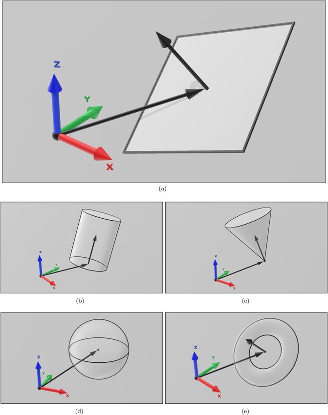
232 Torbjørn L. Leirmo and Oleksandr Semeniuta
Figure 2: Shape features with position and orientation vectors. Spheres are not assigned an orientation due to three full degrees of freedom
in rotation. (a) Plane with position and orientation vector. (b) Cylinder with position and orientation vector. (c) Cone with position and
orientation vector. (d) Sphere with only position vector. (e) Torus with position and orientation vector.
spheres, cones, and tori. The quality of each feature ∑ni = 1QiAi
Qpart = , (5)
type can be modeled as a function of some parameters Apart
Q F = f (x1, x2 , … , xn). If a consistent measure of quality is where n is the number of features, Qi and Ai are the
applied (e.g., surface roughness Ra), the mean quality of quality and area of the ith feature, respectively, and
the entire part Qpart may be calculated as follows: Apart is the total surface area of the part.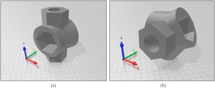
Minimizing form errors in additive manufacturing with part build orientation 233
While the area may be a suitable weight factor in →
This means that the orientation vector v of a feature
many cases, it is also possible to introduce a separate may be expressed as follows:
weight factor that enables the prioritization of features.
This weight factor can be applied on any level, e.g., cer- ⎡ x cos β cos γ + y (sin α sin β cos γ − sin γ cos α) ⎤
tain feature types may be ignored, or individual features ⎢ ⎥
⎢ + z (sin α sin γ + sin β cos α cos γ ) ⎥
may attain a higher priority. Furthermore, the funda- → ⎢
v = x sin γ cos β + y (sin α sin β sin γ + cos α cos γ ) ⎥, (10)
mental assumption is made that the quality of an addi- ⎢ ⎥
⎢ + z ( −sin α cos γ + sin β cos γ cos α) ⎥
tively manufactured surface can be described as a function ⎢ ⎥
of its orientation with respect to the build direction. ⎢
⎣ − x sin β + y sin α cos β + z cos α cos β ⎥
⎦
The orientation of a feature F with respect to the which means
build direction ẑ may be described as two Euler angles
(α, β ) necessary for the rotational transformation of ẑ to → (11)
vz = −x sin β + y sin α cos β + z cos α cos β .
→ →
v where v is the feature vector of F . In the current work,
(α, β ) represents rotations about the x - and y -axis respec- →
When vz from equation (11) is inserted in equation
tively, both with reference to the original reference frame (7), the final expression simply becomes
(i.e., Tait-Brian angles X1Y2Z3 ).
→ → θ = arccos( −x sin β + y sin α cos β + z cos α cos β ) . (12)
The angle θ between two arbitrary vectors u and v is
found by: To enable the mathematical description of the entire
geometry in a single expression, the orientation of each
→ →
⎛u ⋅ v ⎞ feature is described relative to a common coordinate
θ = arccos ⎜ → → ⎟ . (6)
frame, i.e., the WCS. The geometry may be regarded as
⎝ ∣u∣ ⋅∣v∣ ⎠
a rigid body, which means that the relation between the
→ →
By utilizing unit vectors, ∣u∣ ⋅∣v∣ evaluates to 1 and surfaces remains constant and any transformation acts
reduces the expression to on all surfaces equally. In consequence, the orientation
→ → of all surfaces may be collectively calculated from the
θ = arccos( u ⋅ v ) . (7)
same values of α , β , and γ using equation (10), where
→ x , y , and z are the components of the feature’s initial
By inserting ẑ = [0 0 1] for u , the aforementioned
expression can be further reduced because orientation vector. Accordingly, equation (12) is valid
for all surfaces with α and β as the only variables.
x
⎡ ⎤
[0 0 1] ⋅ ⎢ y ⎥ = z . (8)
⎣z⎦
In this context, z will be the z -component of the fea- 3.2 Finding the optimal part build
→ →
ture vector v , denoted vz . However, we want to express orientation
the angle θ as a function of the part’s orientation in 3D
space to enable optimization of orientation. For this pur-
Based on the aforementioned theory, it is possible to
pose, the orientation vector can be expressed in terms of
determine the optimal part build orientation mathemati-
Tait-Bryan angles (Z1Y2X3). These rotations are commonly
cally by evaluating the critical points of the objective
referred to as yaw, pitch, and roll in engineering applica- function. The critical points of a function f (x , y ) are
tions and describes the orientation of a rigid body with found, where
respect to the world coordinate system (WCS). The feature
vector can then be derived from the rotation matrices in ∂f ∂f
= = 0 or undefined . (13)
equations (2)–(4), and the sequential rotations about the ∂x ∂y
x -, y -, and z -axis can then be performed in a single opera- Typically, there will be several solutions to equation
tion by multiplying the matrices as follows: (13), and each solution needs to be evaluated separately.
⎡ cos β cos γ sin α sin β cos γ − sin γ cos α sin α sin γ + sin β cos α cos γ ⎤
R = Rz ⋅ Ry ⋅ Rx = ⎢ sin γ cos β sin α sin β sin γ + cos α cos γ −sin α cos γ + sin β cos γ cos α ⎥. (9)
⎢ ⎥
⎣ −sin β sin α cos β cos α cos β ⎦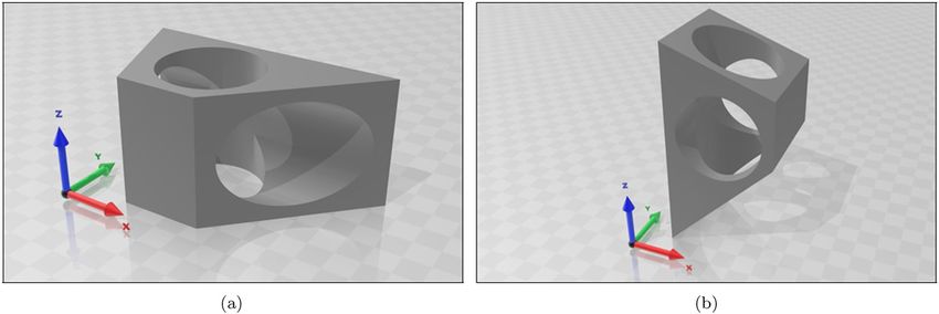
234 Torbjørn L. Leirmo and Oleksandr Semeniuta
selection of significant features and automatic filtering
of features based on type, size, etc.
As surfaces are affected differently by build direction,
separate models for each feature type are necessary to
enable proper evaluation. This is easily implemented by
inserting the appropriate expression for FQuality into equa-
tion (5) for each feature.
4 Case study
Two case studies are presented to demonstrate the pro-
posed method:
Figure 3: Sample part 1 recreated from the study by Cheng et al. [9]
(1) A simple geometry to enable a step-by-step demon-
with coordinate frames.
stration of the approach and all calculations.
(2) A slightly more complex geometry to illustrate the
These solutions will represent points, edges, and perhaps applicability to more complex parts.
even entire areas in the 2D solution space. Provided the
formalization in the previous section, the part build Simple mathematical models of quality are constructed
orientation can be described as a set of two rotations α for the illustrative purpose of this study. The implementa-
and β . If a function is based on these two rotations, α and tion of empirical models is left for future work as this would
β will replace x and y in equation (13) in the search for obscure the central elements of this article. Before the case
critical points. The solution space will be the surface of studies are presented, the construction of these mathema-
a unit sphere, where α ∈ [0, 2π ) and β ∈ [0, π ). A point tical models is detailed to provide the necessary founda-
on this surface will correspond to a single unique orien- tions for the subsequent illustrations.
tation, while a line will correspond to a range of orienta-
tions. Note that the entire unit sphere is accessible already
with only half a rotation of β , and still, a full rotation of β 4.1 Constructing the mathematical models
is used in the visualizations of this article to make their
analysis more intuitive. The following models are based on the orientation rules
The fundamental assumption remains that the quality described by Frank and Fadel [32], stating that cylinders
of a surface can be modeled as a function of its orientation should be oriented with the axis parallel to the build
with respect to the build orientation and that this function direction, while planes can be oriented either parallel
is differentiable. A conditional function (such as the one in or perpendicular to the build direction. Up-facing and
equation (1)) introduces certain challenges to this method. down-facing surfaces are treated equally in the examples
However, such discontinuities would represent edges and to keep the objective functions simple. This can be natu-
areas in the 2D solution space that could be added to the rally incorporated in the objective function to account for
list of candidate orientations. any additional effects, e.g., overcure, support structures,
Each feature of the geometry will add a term to the and so on.
objective function, and each term will typically add one The central assumption in the current work is that the
or more candidate orientations to the list. The exact accuracy of a feature can be modeled as a function of its
number of additional candidates depends on the mathe- angle to the build direction (θ ), which in turn is a func-
matical model as higher order functions will yield more tion of the part’s orientation as described in equation (12).
candidates. It is therefore beneficial to limit or minimize Also, we are modeling deviations from nominal geo-
the number of terms to avoid excessive computations. A metry, which can be considered a cost; hence, a low
simple way to minimize the number of terms is to join cost indicates a high fitness of a given orientation. How-
similar terms, e.g., two features of the same type and ever, the angle will not be sufficient to evaluate the fit-
orientation can be combined into a single term of the ness of a certain orientation. Consider, for instance, a
objective function. Other measures include a manual cylinder oriented at a 45 ∘ angle from the build direction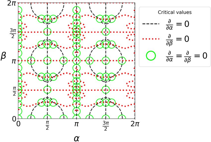
Minimizing form errors in additive manufacturing with part build orientation 235
Figure 4: Solution spaces for planes and cylinders α , β ∈ [0, 2π ] from equations (15) and (17), respectively. (a) 3D-graph for cylinders.
(b) Contour for cylinders. (c) 3D graph for planes. (d) Contour for planes.
Table 3: Numeric description of part features for sample part 1
Position Orientation Area
# Type Px Py Pz Ex Ey Ez mm2 %
1 Plane 4.55 0.00 1.80 0.00 −1.00 0.00 20 9.3
2 Plane 5.00 2.50 0.00 0.00 0.00 −1.00 50 22.8
3 Plane 3.41 2.50 5.00 0.00 0.00 1.00 16 7.3
4 Plane 4.55 5.00 1.80 0.00 1.00 0.00 20 9.3
5 Plane 0.91 2.50 2.50 −0.90 0.00 0.45 13 6.0
6 Plane 7.50 2.50 2.50 0.81 0.00 0.59 18 8.0
7 Cylinder 4.00 0.00 2.50 0.00 1.00 0.00 31 14.0
8 Cylinder 0.18 2.50 2.50 1.00 0.00 0.00 51 23.1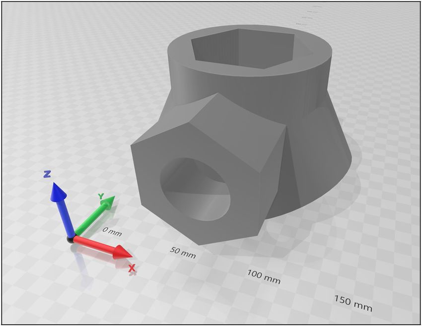
236 Torbjørn L. Leirmo and Oleksandr Semeniuta
Figure 5: Solution space for case 1 based on equation (19). (a) 3D-graph for case 1. (b) Contour for case 1.
(θ = 45 ∘ ). The same cylinder oriented at θ = 135 ∘ would where θ is the angle between the feature normal vector
yield the same result, but the angle θ is quite different. and the build direction. This can be formulated as a func-
Clearly, the objective function should be more sophisti- tion of (α, β ) by inserting equation (12) for θ . With this
cated to incorporate this behavior. substitution for θ , equation (14) may be written as
Because the angle θ always will be in the interval follows:
[0 ∘ , 180 ∘ ], the sine of the angle will provide three desir-
Qcylinder (α, β )
able properties of an objective function: (i) the result (15)
is always a number between 0 and 1, (ii) the function = 1 − ( −x sin β + y sin α cos β + z cos α cos β )2 .
is minimized at vertical orientations and maximized at
Planes, on the other hand, require some additional
horizontal orientations, and (iii) the function is periodic
configurations as we must consider both vertical and
and symmetric. This study employs this function as an
horizontal orientations as positive. To incorporate this
expression for the quality of cylinders:
new behavior, equation (14) is multiplied by cos2 θ . This
Qcylinder (θ ) = sin θ , (14) term ensures that planes are positively evaluated at both
∂ ∂
Figure 6: Graphs displaying the partial derivatives of equation (19). (a) Contour for ∂α
. (b) Contour for ∂β
.Minimizing form errors in additive manufacturing with part build orientation 237
Qplane(α, β )
= 2.598 1 − ( −x sin β + y sin α cos β + z cos α cos β )2
× ( −x sin(β ) + y sin(α) cos(β ) + z cos(α) cos(β ))2 .
(17)
The solution spaces of equations (15) and (17) are
illustrated in Figure 4, where a 3D graph and a contour
plot are presented for each of the equations.
4.2 Case 1: A simple geometry
Figure 7: Contour lines for the partial derivatives of equation (19). The first case study is the simple geometry reconstructed
from the study by Cheng et al. [9] and presented in Figure 3.
This geometry provides a gentle introduction to the method
vertical and horizontal orientations. In addition, the by enabling a step-wise analysis of the geometry and the
function is more sensitive to minor changes when a accuracy model. The first step of the method is to obtain a
plane is horizontal than when the plane is vertical. numeric description of the geometry in the appropriate
This fit well together with the VE being large when the format. Table 3 provides the positions and orientations of
plane is close to horizontal, while not being as promi- the features defined relative to the PCS as illustrated in
nent in close-to-vertical orientations. Figure 3.
Finally, the function is normalized to facilitate com- The data from Table 3 are inserted into equations (15)
parison with other feature types, and so on. The normal- and (17) one row at a time as follows:
ization is achieved by introducing a divisor equal to (1) The feature type determines which equation to use
the maximum of the function. The maximum is easily (equation (15) for cylinders or equation (17) for
obtained by derivation and reveals a normalization factor planes)
of 2.598 when rounded to three decimal points. This (2) The variables x , y , and z are substituted with Ex , Ey ,
yields the following expression for the quality of planes: and Ez from Table 3
Qplane(θ ) = 2.598 sin θ cos2 θ , (16) (3) The expression is multiplied with the relative surface
area of the feature (final column of Table 3)
where θ is the angle between the feature normal vector
and the build direction. As with equation (14), the expres- Following the progression mentioned earlier, we start
sion for planes may also be rewritten as a function of with the first row from Table 3 and perform the following
(α, β ) by inserting equation (12) for θ . The result may be steps: (1) The feature is identified as a planar type, and we,
formulated as follows: therefore, use equation (17). (2) The values of Ex , Ey , and Ez
Table 4: Evaluation of critical points for case 1
0 ∘ ≤ α < 45 ∘ 45 ∘ ≤ α < 180 ∘ 180 ∘ ≤ α < 225 ∘ 225 ∘ ≤ α < 360 ∘
Orientation Cost Orientation Cost Orientation Cost Orientation Cost
(0, 0) 0.46 (87, 40) 0.53 (180, 0) 0.46 (267, 140) 0.53
(0, 28) 0.71 (87, 220) 0.53 (180, 28) 0.69 (267, 320) 0.53
(0, 90) 0.26 (90, 0) 0.23 (180, 90) 0.26 (270, 0) 0.23
(0, 152) 0.69 (90, 90) 0.26 (180, 152) 0.71 (270, 90) 0.26
(0, 180) 0.46 (90, 180) 0.23 (180, 180) 0.46 (270, 180) 0.23
(0, 208) 0.71 (90, 270) 0.26 (180, 208) 0.69 (270, 270) 0.26
(0, 270) 0.26 (93, 140) 0.53 (180, 270) 0.26 (273, 40) 0.53
(0, 332) 0.69 (93, 320) 0.53 (180, 332) 0.71 (273, 220 0.53
(38, 176) 0.85 (142, 4) 0.85 (218, 4) 0.85 (322, 176) 0.85
(38, 356) 0.85 (142, 184) 0.85 (218, 184) 0.85 (322, 356) 0.85
Lower value indicates higher accuracy. Lowest value in bold.238 Torbjørn L. Leirmo and Oleksandr Semeniuta
Figure 8: Optimal orientations identified for case 1. (a) Identified optimum (90 ∘ , 0 ∘ ). (b) Second-best orientation (0 ∘ , 90 ∘ ).
PQuality (α, β )
= 0.23 1 − sin2(β ) + 0.14 1 − sin2(α) cos2 (β )
+ 0.48 1 − sin2(α) cos2 (β ) sin2(α) cos2 (β )
+ 0.78 1 − cos2 (α) cos2 (β ) cos2 (α) cos2 (β )
(19)
+ 0.10 1 − 0.5( − sin(β ) + cos(α) cos(β ))2
× ( −sin(β ) + cos(α) cos(β ))2
+ 0.14 1 − 0.88(sin(β ) + 0.36 cos(α) cos(β ))2
× (sin(β ) + 0.36 cos(α) cos(β ))2 .
This yields the solution space illustrated in Figure 5.
The solution space reflects the symmetry and regularity
of the geometry as the orientations where feature vectors
align with the build direction are clear.
Figure 9: The joint designed for case 2. In the next step, the partial derivatives are calculated
and evaluated according to equation (13). Figure 6 shows
are inserted for x , y and z , respectively. For the first fea- the graphs of the partial derivatives where the dashed
ture, this means that 0 is inserted for x and z , while 1 is lines of Figure 6(a) and (b) correspond to the contour
inserted for y . (3) Finally, the weight factor is introduced lines where the derivative evaluates to zero or are
by multiplying by the relative surface area as found in the undefined.
final column of Table 3, namely, 0.093 (9.3%). These steps The critical points are found where both derivatives
are displayed in the calculations of equation (18). either evaluate to zero or are undefined. This can be
displayed graphically by plotting the dashed lines of
Q F1(α, β )
Figure 6(a) and (b) in a single figure as shown in Figure 7.
= 2.598A 1 − ( −x sin β + y sin α cos β + z cos α cos β )2 Finally, individual evaluation of these points and edges
× ( −x sin(β ) + y sin(α) cos(β ) + z cos(α) cos(β ))2 must be conducted to identify the global optimum as
= 2.598A 1 − ( −0 sin β + 1 sin α cos β + 0 cos α cos β )2 tabulated in Table 4.
The evaluation of α, β ∈ [0, 2π ) reveals four solutions
× ( −0 sin(β ) + 1 sin(α) cos(β ) + 0 cos(α) cos(β ))2
with equal cost. However, these four solutions are pair-
= 2.598 × 0.093 1 − sin2(α) cos2 (β ) sin2(α) cos2 (β ) wise identical, i.e., (270 ∘ , 180 ∘ ) is the same as (90 ∘ , 0 ∘ ),
= 0.24 1 − sin2(α) cos2 (β ) sin2(α) cos2 (β ) . and (90 ∘ , 180 ∘ ) is the same as (270 ∘ , 0 ∘ ). Moreover,
these two unique orientations are polar opposites, corre-
(18)
sponding to the object lying on its left or right side as
When all the data from Table 3 are inserted into equa- exemplified in Figure 8(a). This evaluation of the optimal
tions (15) and (17), all the equations may be collected in a orientation is also consistent with previous assessments
single expression for the entire geometry as follows: of the same geometry [9,11,16].Minimizing form errors in additive manufacturing with part build orientation 239
Table 5: Numeric description of features for sample part 2
Position Orientation Area
# Type Px Py Pz Ex Ey Ez mm2 %
1 Plane 32.14 0.00 −64.83 0.89 0.00 −0.45 6,176 6.26
2 Plane −32.14 0.00 −64.83 −0.89 0.00 −0.45 6,176 6.26
3 Plane 0.00 0.00 25.00 0.00 0.00 1.00 3,697 3.75
4 Plane 0.00 84.64 −25.00 0.00 1.00 0.00 2,900 2.94
5 Plane 0.00 −84.64 −25.00 0.00 −1.00 0.00 2,900 2.94
6 Plane 15.56 0.00 −17.22 −0.89 0.00 0.45 2,324 2.35
7 Plane −15.56 0.00 −17.22 0.89 0.00 0.45 2,324 2.35
8 Plane 0.00 34.64 2.41 0.00 −1.00 0.00 1,800 1.82
9 Plane 0.00 −34.64 2.41 0.00 1.00 0.00 1,800 1.82
10 Plane 34.64 62.85 −24.18 1.00 0.00 0.00 1,735 1.76
11 Plane 34.64 −62.85 −24.18 1.00 0.00 0.00 1,735 1.76
12 Plane −34.64 62.85 −24.18 −1.00 0.00 0.00 1,735 1.76
13 Plane −34.64 −62.85 −24.18 −1.00 0.00 0.00 1,735 1.76
14 Plane 18.32 64.93 4.43 0.50 0.00 0.87 1,560 1.58
15 Plane 18.32 −64.93 4.43 0.50 0.00 0.87 1,560 1.58
16 Plane −18.32 64.93 4.43 −0.50 0.00 0.87 1,560 1.58
17 Plane −18.32 −64.93 4.43 −0.50 0.00 0.87 1,560 1.58
18 Plane 17.43 66.74 −54.94 0.50 0.00 −0.87 1,430 1.45
19 Plane 17.43 −66.74 −54.94 0.50 0.00 −0.87 1,430 1.45
20 Plane −17.43 66.74 −54.94 −0.50 0.00 −0.87 1,430 1.45
21 Plane −17.43 −66.74 −54.94 −0.50 0.00 −0.87 1,430 1.45
22 Plane 29.52 18.15 7.38 −0.87 −0.50 0.00 1,400 1.42
23 Plane 29.52 −18.15 7.38 −0.87 0.50 0.00 1,400 1.42
24 Plane −29.52 18.15 7.38 0.87 −0.50 0.00 1,400 1.42
25 Plane −29.52 −18.15 7.38 0.87 0.50 0.00 1,400 1.42
26 Plane 14.47 24.49 −28.94 0.89 0.00 −0.45 314 0.32
27 Plane 14.47 −24.49 −28.94 0.89 0.00 −0.45 314 0.32
28 Plane −14.47 24.49 −28.94 −0.89 0.00 −0.45 314 0.32
29 Plane −14.47 −24.49 −28.94 −0.89 0.00 −0.45 314 0.32
30 Cylinder 0.00 0.00 −7.68 0.00 0.00 1.00 7,590 7.69
31 Cylinder 0.00 0.00 −25.00 −0.89 0.00 −0.45 6,804 6.89
32 Cylinder 0.00 0.00 −25.00 0.89 0.00 −0.45 6,804 6.89
33 Cylinder 0.00 50.00 −25.00 0.00 1.00 0.00 4,518 4.58
34 Cylinder 0.00 −50.00 −25.00 0.00 −1.00 0.00 4,518 4.58
35 Cylinder 14.47 24.49 −28.94 0.89 0.00 −0.45 2,513 2.55
36 Cylinder 14.47 −24.49 −28.94 0.89 0.00 −0.45 2,513 2.55
37 Cylinder −14.47 24.49 −28.94 −0.89 0.00 −0.45 2,513 2.55
38 Cylinder −14.47 −24.49 −28.94 −0.89 0.00 −0.45 2,513 2.55
39 Cylinder 0.00 0.00 −25.00 0.00 0.00 1.00 449 0.45
40 Cylinder 0.00 0.00 −25.00 0.00 0.00 1.00 449 0.45
41 Cylinder 0.00 0.00 −25.00 −0.89 0.00 −0.45 411 0.42
42 Cylinder 0.00 0.00 −25.00 −0.89 0.00 −0.45 411 0.42
43 Cylinder 0.00 0.00 −25.00 0.89 0.00 −0.45 411 0.42
44 Cylinder 0.00 0.00 −25.00 0.89 0.00 −0.45 411 0.42
Another orientation achieving a low cost is the upright largest cylinder with the build direction as displayed in
position which is achieved for any value of α when β is 90 ∘ Figure 8(b). Note that the up-facing and down-facing sur-
or 270 ∘ . This constitutes two edges in the solution space faces are not differentiated by the objective function.
with identical solutions. These orientations correspond to Incorporating this behavior would yield different results
the front or the back facing upwards, which aligns the where repetition of the solution space is avoided.240 Torbjørn L. Leirmo and Oleksandr Semeniuta
Figure 10: Solution space for case 2 based on equation (20). (a) 3D graph for case 2. (b) Contour for case 2.
∂ ∂
Figure 11: Graphs displaying the partial derivatives of equation (20). (a) Contour for ∂α
. (b) Contour for ∂β
.
4.3 Case 2: Example with more complex
geometry
The second case is an original design created for the sole
purpose of demonstrating the applicability of the pro-
posed method on a slightly more complex geometry.
The part displayed in Figure 9 is a joint with connectors
in various directions. Forty-four features may be identi-
fied where 15 are cylindrical, and the remaining 29 are
planes. A numeric description of the geometry is pre-
sented in Table 5.
Using the functions for planes and cylinders from
equations (15) and (17) populated with the data of Table 5,
the solution space of Figure 10 is obtained. Because many Figure 12: Contour lines for the partial derivatives of equation (20).Minimizing form errors in additive manufacturing with part build orientation 241
features share orientation vectors, the overall objective function can be simplified to contain a minimal number of
terms.
PQuality (α, β ) = 0.18 cos2 (β ) sin2(β ) + 0.09 1 − cos2 (α) cos2 (β ) + 0.09 1 − sin2(α) cos2 (β )
+ 0.25 1 − sin2(α) cos2 (β ) sin2(α) cos2 (β ) + 0.10 1 − cos2 (α) cos2 (β ) cos2 (α) cos2 (β )
+ 0.13 1 − 0.8(sin(β ) − 0.5 cos(α) cos(β ))2 + 0.12 1 − 0.8(sin(β ) + 0.5 cos(α) cos(β ))2
+ 0.14 1 − 0.8(sin(β ) − 0.5 cos(α) cos(β ))2 (sin(β ) − 0.5 cos(α) cos(β ))2
+ 0.05 1 − 0.8(sin(β ) + 0.5 cos(α) cos(β ))2 (sin(β ) + 0.5 cos(α) cos(β ))2
+ 0.14 1 − 0.8(sin(β ) + 0.5 cos(α) cos(β ))2 (sin(β ) + 0.5 cos(α) cos(β ))2
+ 0.03 1 − 0.75(0.58 sin(α) cos(β ) − sin(β ))2 (0.58 sin(α) cos(β ) − sin(β ))2 (20)
+ 0.06 1 − 0.75(0.58 sin(α) cos(β ) + sin(β ))2 (0.58 sin(α) cos(β ) + sin(β ))2
+ 0.05 1 − 0.8( − sin(β ) + 0.5 cos(α) cos(β ))2 (sin(β ) − 0.5 cos(α) cos(β ))2
+ 0.06 1 − 0.75(0.58 sin(β ) − cos(α) cos(β ))2 (0.58 sin(β ) − cos(α) cos(β ))2
+ 0.12 1 − 0.75(0.58 sin(β ) + cos(α) cos(β ))2 (0.58 sin(β ) + cos(α) cos(β ))2
+ 0.03 1 − 0.75( − 0.58 sin(α) cos(β ) + sin(β ))2 (0.58 sin(α) cos(β ) − sin(β ))2
+ 0.06 1 − 0.75( − 0.58 sin(β ) + cos(α) cos(β ))2 (0.58 sin(β ) − cos(α) cos(β ))2
The solution space for the second case is also quite becomes more favorable than the previous best at
regular as demonstrated in Figure 11 where the partial (90 ∘ , 0 ∘ ) (see Figure 13(b)). This analysis indicates that
derivatives of equation (20) are displayed. The regularity for this part, cylinders should be at least 3.4 times as
of these plots reflects the redundancy in the domain important relative to planes before the orientation at
α, β ∈ [0, 2π ]. (0 ∘ , 63 ∘ ) is selected.
As demonstrated in case 1, the critical points are found Both case studies exhibit repetitive symmetric pat-
where both partial derivatives are either zero or undefined, terns in the evaluation table. This symmetry arises from
which corresponds to the intersections of red and black two sources: (i) as stated in Section 2.2, the domain of β
lines in Figure 12. All critical points are tabulated in Table 6 can be constrained to [0, π ) as rotations exceeding this
where the minima are highlighted in bold text. range will only repeat previous solutions, and (ii) the
For the second case study, the optimal orientation is objective function of these case studies takes no regard
achieved by 90 ∘ rotation about the x -axis as displayed in of the difference between up-facing and down-facing
Figure 13(a). The same cost is also observed for three surfaces. One may also question the alignment of many
other combinations of rotations as displayed in Table 6. critical points with right-angle orientations. This is, how-
Due to redundancy in the solution space, these four com- ever, a result of the initial orientation of the part, which
binations of rotations only correspond to two unique originates from the design phase. If the initial orientation
orientations in exactly opposite directions. With the hex- was different, the patterns observed in the plots would
agonal protrusions oriented parallel to the build direc- change due to the projection, but the solution space
tion, 25 out of the 29 planes are in a favorable orientation, would remain unaltered.
while only two of the 15 cylinders are vertical. A more complex geometry with more features would
Clearly, the large number of planes favors the orien- yield a solution space with more local extremes where the
tation at (90 ∘ , 0 ∘ ). However, if cylinders are given a complexity of the solution space reflects the complexity
higher priority than planes, this orientation may no of the geometry. Naturally, the objective functions for
longer be as favorable. Figure 14 compares the effect of each surface type also contribute toward the topology
assigning a weight factor to cylindrical features for three of the solution space. Consequently, different objective
orientations. A point of intersection is identified at a functions, e.g., those obtained through experiments, would
weight factor of 3.4, where the orientation (0 ∘ , 63 ∘ ) give different results to those reported earlier.242 Torbjørn L. Leirmo and Oleksandr Semeniuta
Table 6: Evaluation of critical points for case 2
α = 0∘ 0 ∘ < α < 180 ∘ α = 180 ∘ 180 ∘ < α < 360 ∘
Orientation Cost Orientation Cost Orientation Cost Orientation Cost
(0, 0) 0.53 (40, 0) 0.65 (180, 0) 0.53 (220, 0) 0.65
(0, 23) 0.57 (40, 180) 0.65 (180, 23) 0.57 (220, 180) 0.65
(0, 45) 0.60 (72, 50) 0.72 (180, 45) 0.60 (252, 50) 0.72
(0, 63) 0.54 (72, 130) 0.72 (180, 63) 0.54 (252, 130) 0.72
(0, 81) 0.60 (72, 230) 0.72 (180, 81) 0.60 (252, 230) 0.72
(0, 90) 0.59 (72, 310) 0.72 (180, 90) 0.59 (252, 310) 0.72
(0, 99) 0.60 (90, 0) 0.37 (180, 99) 0.60 (270, 0) 0.37
(0, 117) 0.54 (90, 50) 0.72 (180, 117) 0.54 (270, 50) 0.72
(0, 135) 0.60 (90, 90) 0.59 (180, 135) 0.60 (270, 90) 0.59
(0, 157) 0.57 (90, 130) 0.72 (180, 157) 0.57 (270, 130) 0.72
(0, 180) 0.53 (90, 180) 0.37 (180, 180) 0.53 (270, 180) 0.37
(0, 203) 0.57 (90, 230) 0.72 (180, 203) 0.57 (270, 230) 0.72
(0, 225) 0.60 (90, 270) 0.59 (180, 225) 0.60 (270, 270) 0.59
(0, 243) 0.54 (90, 310) 0.72 (180, 243) 0.54 (270, 310) 0.72
(0, 261) 0.60 (108, 50) 0.72 (180, 261) 0.60 (288, 50) 0.72
(0, 270) 0.59 (108, 130) 0.72 (180, 270) 0.59 (288, 130) 0.72
(0, 279) 0.60 (108, 230) 0.72 (180, 279) 0.60 (288, 230) 0.72
(0, 297) 0.54 (108, 310) 0.72 (180, 297) 0.54 (288, 310) 0.72
(0, 315) 0.60 (140, 0) 0.65 (180, 315) 0.60 (320, 0) 0.65
(0, 337) 0.57 (140, 180) 0.65 (180, 337) 0.57 (320, 180) 0.65
Lower value indicates higher accuracy. Lowest values highlighted in bold.
Figure 13: Optimal orientations identified for case 2. (a) Identified optimum (90 ∘ , 0 ∘ ). (b) Alternative orientation (0 ∘ , 63 ∘ ).
5 Discussion Hence, complex geometries may benefit from intelligent
methods where an effort is made to accelerate the compu-
A mathematical description of the solution space provides tations. The simplicity of an exhaustive search may have
a range of possibilities for finding the optimal orientation. certain advantages for simple geometries but may be inef-
What approach is best suited to solve the optimization fective for complex geometries.
problem depends on the purpose of the optimization as well The continuous solution space facilitates gradient-
as the complexity of the part. As the geometry becomes more based methods as a qualified decision can be made con-
complex, function evaluations are increasingly expensive. cerning the next iteration of the search sequence. However,Minimizing form errors in additive manufacturing with part build orientation 243
The proposed method is not applicable to freeform
surfaces due to the inability to formulate proper objective
functions to handle the unknown. At present, this is not
an issue for assembly features. However, as the potential
of AM is unlocked, more complex surfaces may become
widely used in the industrial design. The development of
flexible formulations to handle this challenge is left for
future work, along with the appropriate parametrization
of such surfaces.
Figure 14: Comparison of three orientations for case part 2 when an
additional weight factor is introduced for cylinders.
6 Conclusions and outlook
unless all critical points are investigated, the risk of getting The approach described in this article provides the math-
stuck in local optima is ever present. A stochastic compo- ematical foundations for both deterministic and stochastic
nent or a larger population of solutions may counter this solutions to the orientation problem. By describing the
problem, as is typically the case of EAs. solution space as a continuous function in a closed domain,
When the solution space is clearly defined, it is pos- the optimization can be performed mathematically. More
sible to identify feasible regions in line with previous importantly, this approach enables the determination of
works [25,18]. These regions are defined from requirements feasible orientation zones for the optimization of secondary
and represent ranges of feasible orientations where toler- objectives. Under the assumption that quality can be des-
ance requirements are met. Consequently, these regions cribed as a function of build direction, the proposed method
can make up the boundaries for subsequent optimizations, can be populated with any mathematical description of the
e.g., with respect to mechanical properties. Adding steps to relationship between quality and part build orientation.
the optimization process will inevitably complicate and pro- The development of accurate mathematical models is
long the process, but interactive methods may be useful crucial for optimization in process planning. AM technol-
when the objectives are fuzzy or when flexibility is required. ogies comprise many different processes that require sepa-
Practical implementations of the proposed method rate models for predicting final part properties. Future
would entail the formulation of objective functions for research entails developing and validating prediction
all relevant surface types. The relevant types and their models that can be utilized in optimization processes.
definition may differ as long as they can be formulated as Practical implementation in a system with capabilities
orientation vectors with accompanying objective func- beyond the described method constitutes an interesting
tions. Furthermore, a solution for obtaining information avenue for future research. Furthermore, the integration
on the orientation of the surfaces is required to automate of all processing stages into a digital pipeline – from
the optimization process. An alternative implementation design and process planning to quality assessment and ver-
enables the identification of feasible regions for subse- ification – will enable traceability throughout the manufac-
quent optimization. This would imply the integration of turing system and ultimately the entire product life cycle.
the method in a larger system with capabilities beyond
what can be expressed by surfaces and their orientations. Acknowledgements: The authors appreciate the support
The proposed optimization method has the benefit of from colleagues at the Department of Manufacturing and
being stable (i.e., no stochastic components), has no lim- Civil Engineering.
itations with regards to search grid resolution, and pro-
vides the flexibility to incorporate separate expressions Funding information: This research is funded by the
for each feature. Moreover, by considering the features of Norwegian Ministry of Research and Education through
the part rather than every facet of a tessellated file, the the PhD-grant of Torbjørn Langedahl Leirmo.
effect of build direction may be generalized for each sur-
face type. This drastically reduces the number of function Author contributions: TLL conceptualized the presented
evaluations. The feature-based approach also enables method with technical and theoretical support from OS.
feature dimensions to be included in the objective func- OS reviewed and edited the original draft put forward
tion, which may affect the outcome. by TLL.You can also read