Including filter-feeding gelatinous macrozooplankton in a global marine biogeochemical model: model-data comparison and impact on the ocean carbon ...
←
→
Page content transcription
If your browser does not render page correctly, please read the page content below
Research article
Biogeosciences, 20, 869–895, 2023
https://doi.org/10.5194/bg-20-869-2023
© Author(s) 2023. This work is distributed under
the Creative Commons Attribution 4.0 License.

Including filter-feeding gelatinous macrozooplankton in a global
marine biogeochemical model: model–data comparison
and impact on the ocean carbon cycle
Corentin Clerc1 , Laurent Bopp1 , Fabio Benedetti2 , Meike Vogt2 , and Olivier Aumont3
1 LMD/IPSL,Ecole normale supérieure/Université PSL, CNRS, Ecole Polytechnique, Sorbonne Université, Paris, France
2 Environmental
             Physics, Institute of Biogeochemistry and Pollutant Dynamics, ETH Zürich, 8092 Zürich, Switzerland
3 LOCEAN/IPSL, IRD, CNRS, Sorbonne Université, MNHN, Paris, France

Correspondence: Corentin Clerc (corentin.clerc@lmd.ens.fr)

Received: 16 November 2022 – Discussion started: 30 November 2022
Revised: 1 February 2023 – Accepted: 7 February 2023 – Published: 28 February 2023

Abstract. Filter-feeding gelatinous macrozooplankton              spatio-temporal variability of FFGM. FFGM substantially
(FFGM), namely salps, pyrosomes and doliolids, are in-            contribute to carbon export at depth (0.4 Pg C yr−1 at
creasingly recognized as an essential component of the            1000 m), particularly in low-productivity regions (up to
marine ecosystem. Unlike crustacean zooplankton (e.g.,            40 % of organic carbon export at 1000 m), where they
copepods) that feed on prey that are an order of magnitude        dominate macrozooplankton biomass by a factor of 2. The
smaller, filter feeding allows FFGM to have access to a           FFGM-induced export increases in importance with depth,
wider range of organisms, with predator-over-prey size            with a simulated transfer efficiency close to 1.
ratios as high as 105 : 1. In addition, most FFGM produce
carcasses and/or fecal pellets that sink 10 times faster than
those of copepods. This implies a rapid and efficient export
of organic matter to depth. Even if these organisms represent     1   Introduction
< 5 % of the overall planktonic biomass, their associated
organic matter flux could be substantial. Here we present         Pelagic tunicates, i.e., salps, doliolids, pyrosomes and appen-
a first estimate of the influence of FFGM on the export of        dicularians, are free-swimming open-ocean gelatinous zoo-
particulate organic matter to the deep ocean based on the         plankton that are increasingly recognized as key components
marine biogeochemical model NEMO-PISCES (Nucleus                  of marine ecosystems and biogeochemical cycles (Henschke
for European Modelling of the Ocean, Pelagic Interaction          et al., 2016; Luo et al., 2020). All pelagic tunicates, with
Scheme for Carbon and Ecosystem Studies). In this new             the exception of appendicularians, are part of the macrozoo-
version of PISCES, two processes characterize FFGM:               plankton (> 2 mm) and are filter-feeding organisms. Here-
the preference for small organisms due to filter feeding          after they will be referred to as filter-feeding gelatinous
and the rapid sinking of carcasses and fecal pellets. To          macrozooplankton (FFGM). FFGM, which are urochordates,
evaluate our simulated FFGM distribution, we compiled             are water-rich free-swimming transparent animals. There-
FFGM abundance observations into a monthly biomass                fore, although they are not part of the same phyla, they have
climatology using a taxon-specific biomass–abundance              been placed in the same functional group as ctenophores and
conversion. Model–observation comparison supports the             cnidarians (jellyfish), i.e., gelatinous zooplankton (GZ).
model’s ability to quantify the global and large-scale patterns      The fragility of all GZ bodies partly explains the rar-
of FFGM biomass distribution but reveals an urgent need to        ity of observations (Henschke et al., 2016). Nevertheless, it
better understand the factors triggering the boom-and-bust        has been hypothesized that increasing anthropogenic pres-
FFGM dynamics before we can reproduce the observed                sures on the global ocean favor gelatinous zooplankton in
                                                                  most regions due to eutrophication, overfishing or climate

Published by Copernicus Publications on behalf of the European Geosciences Union.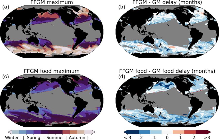
870                                                                 C. Clerc et al.: FFGM impacts on the ocean carbon cycle

change (Richardson et al., 2009; Purcell, 2012). Research ef-       impact and the nature of their carcasses and fecal pellets re-
fort focusing on GZ has increased dramatically over the last        mains very limited (Décima et al., 2019). Intense carcass-fall
2 decades, particularly on cnidarians (“true jellyfish”) that       events have been described as responsible for large carbon
contribute significantly to biological carbon cycling through       exports due to their high carbon content (35 % DW, one of
“jelly falls” (i.e., the accumulation of gelatinous zooplankton     the highest among GZ; Lebrato and Jones, 2009). Although
carcasses in the water column following a swarming event;           their fecal pellets sink 30 times slower than those of large
Lebrato et al., 2012; Sweetman et al., 2014; Sweetman and           salps (70 m d−1 according to Drits et al., 1992), they are able
Chapman, 2015; Luo et al., 2020). Similarly, recent studies         to export a significant amount of carbon in addition to ac-
have also focused on pelagic tunicates (namely salps (e.g.,         tive transport through diurnal vertical migrations (Stenvers
Phillips et al., 2009; Henschke et al., 2021a, b; Lüskow et al.,    et al., 2021; Henschke et al., 2019). Because of their rapidly
2020; Ishak et al., 2020; Stone and Steinberg, 2016), ap-           sinking fecal pellets (over 400 m d−1 ) and high clearance
pendicularians (e.g., Berline et al., 2011) and doliolids (e.g.,    rates, doliolids also affect carbon fluxes (Takahashi et al.,
Stenvers et al., 2021)), revealing their importance in carbon       2013, 2015; Ishak et al., 2020), but their impact remains
cycling and for the ecosystem structure, at least on a regional     poorly documented.
scale. Yet, despite this growing interest, the importance of           Overall, most studies to date have focused on regional
FFGM at the global scale remains uncertain.                         scales. Recently, Luo et al. (2020) have estimated the contri-
   Pelagic tunicates are capable of swarming, which means           bution to the global carbon cycle of three categories of gelati-
that their population can reach a high abundance in a very          nous zooplankton: ctenophores, cnidarians and pelagic tuni-
short time and can therefore represent a significant part of        cates. Using a data-driven carbon cycle model, they found
and even dominate the zooplankton community during mas-             that pelagic tunicates contribute three quarters of the partic-
sive proliferation events (Everett et al., 2011; Henschke et al.,   ulate organic carbon (POC) flux induced by gelatinous zoo-
2016). Three mechanisms have been hypothesized to trig-             plankton or one quarter of the total POC exported at 100 m.
ger these swarms: (i) FFGM use a mucus structure to filter          A more recent study by the same team (Luo et al., 2022)
feed, which gives them access to a wide range of preys, from        revised this estimate to 0.57 Pg C yr−1 , representing 9 % of
bacteria to mesozooplankton (Acuña, 2001; Sutherland et al.,        total export at 100 m, by explicitly representing FFGM in the
2010; Bernard et al., 2012; Ambler et al., 2013; Sutherland         COBALT-v2 biogeochemical model (FFGM refers to large
and Thompson, 2022). This feeding strategy might allow              pelagic tunicates in their study).
them to proliferate in response to the bloom of a wide variety         Marine biogeochemical models have repeatedly shown
of organisms, which is in contrast to typical zooplankton with      their usefulness in understanding marine processes on a
prey-to-predator size ratios ranging from 1 : 10 to 1 : 100         global scale, particularly for the role of plankton in ecosys-
(Hansen et al., 1994); (ii) FFGM generally have high clear-         tem processes (e.g., Sailley et al., 2013; Le Quéré et al.,
ance and growth rates (Alldredge and Madin, 1982; Hen-              2016; Kearney et al., 2021) and biogeochemical fluxes (e.g.,
schke et al., 2016) that promote rapid proliferation. The dens-     Buitenhuis et al., 2006; Kwiatkowski et al., 2018; Aumont
est FFGM swarms can sweep over 200 % of their resident              et al., 2018). Their complexity has been increased by the
water volume per day (Ishak et al., 2020). (iii) Some FFGM,         addition of multiple limiting nutrients and multiple func-
such as salps, have life cycles characterized by the alterna-       tional groups or size classes of phytoplankton and zooplank-
tion between a sexual phase (the blastozooid) and an asexual        ton (e.g., Le Quéré et al., 2005; Follows et al., 2007; Ward
phase (the oozoid). During the asexual phase, oozoids pro-          et al., 2012; Aumont et al., 2015). Notably, plankton func-
duce long chains of blastozooid clones that can number sev-         tional type (PFT) models have been introduced as a way of
eral hundreds of individuals and give rise to swarming pro-         grouping organisms that keeps the overall biological com-
cesses (Loeb and Santora, 2012; Kelly et al., 2020; Groen-          plexity at a manageable level (Moore et al., 2001; Gregg
eveld et al., 2020). Based on their potential to form large         et al., 2003; Le Quéré et al., 2005). Wright et al. (2021)
swarms, FFGM can significantly affect ecological processes,         showed that the introduction of a jellyfish PFT (cnidarians
at least locally.                                                   only) into the PlankTOM model has a large direct influ-
   FFGM could also have an impact on the ocean carbon               ence on the biomass distribution of the crustacean macrozoo-
cycle. Indeed, many FFGM produce fast sinking carcasses             plankton PFT and indirectly influences the biomass distri-
and/or fecal pellets that induce a very efficient carbon ex-        butions of protozooplankton and mesozooplankton through
port, especially during swarming events (Henschke et al.,           a trophic cascade. This influence could be explained by the
2016). Large fecal pellets and carcasses of salps are carbon        specific diet of jellyfish that differs from other zooplankton
rich (more than 30 % of dry weight (DW)) and sink at speeds         PFTs. Similarly, the inclusion of FFGM as a new PFT in a
up to 2700 m d−1 for fecal pellets and 1700 m d−1 for car-          PFT-based model has been recently achieved by Luo et al.
casses (Henschke et al., 2016; Lebrato et al., 2013). In ar-        (2022). In their study, they introduced two tunicates groups
eas where salps proliferate, they can induce a carbon trans-        into the COBALT-v2 model – a large salps and doliolids
fer to the seafloor 10 times faster than that in their absence      (FFGM) group and a small appendicularian group – and esti-
(Henschke et al., 2016). For pyrosomes, knowledge on their

Biogeosciences, 20, 869–895, 2023                                                       https://doi.org/10.5194/bg-20-869-2023
C. Clerc et al.: FFGM impacts on the ocean carbon cycle                                                                            871

mated their impact on the surface carbon cycle, but they did
not consider the impacts on the deeper carbon cycle.
   Here, we use the PISCES-v2 model (Aumont et al., 2015),
which is the standard marine biogeochemistry component
of NEMO (Nucleus for European Modelling of the Ocean).
In this study, a new version of PISCES was developed
(PISCES-FFGM) in which two new PFTs were added: a
generic macrozooplankton (GM) based on an allometric scal-
ing of the existing mesozooplankton and a filter-feeding
gelatinous macrozooplankton (FFGM). Two processes char-
acterize FFGM in this version of the model: access to a wide
range of preys through filter feeding and rapid sinking of car-
casses and fecal pellets. We first examine how the model suc-
ceeds in reproducing the surface distribution of FFGM by
providing a new compilation of abundance observations con-
verted to carbon biomass via taxon-specific conversion func-
tions to make this assessment. Second, because the modeling
study by Luo et al. (2022) focused on the impact of FFGM
on surface processes, we investigated whether our modeling
framework and formulations produce results consistent with
theirs. Our study also provides some new insights: (1) we           Figure 1. Architecture of PISCES-FFGM. This figure only shows
explore the FFGM-specific spatial patterns of organic matter        the organic components of the model, thus omitting oxygen and
production, export and particle composition in the top 100 m;       the carbonate system. This diagram emphasizes trophic interac-
                                                                    tions (turquoise arrows, the width representing the preference of
(2) we investigate the impacts of FFGM on the export of par-
                                                                    the predator for the prey) and particulate organic matter production
ticulate organic carbon to the deep ocean via an explicit rep-      (black arrows), two processes strongly impacted by the introduction
resentation of fast-sinking fecal pellets and carcasses.            of two new zooplankton groups in PISCES-FFGM (pink boxes).
                                                                    FFGM is for filter-feeding gelatinous macrozooplankton; GM is for
                                                                    generic macrozooplankton; POM is for particulate organic matter;
2     Materials and method                                          DOM is for dissolved organic matter.

2.1     Model description
                                                                    spectively (GM carcasses, GM fecal pellets, FFGM carcasses
2.1.1    Model structure                                            and FFGM fecal pellets; see Fig. 1). Because both macro-
                                                                    zooplankton groups have a constant Fe : C stoichiometry and
The marine biogeochemical model used in the present study           feed on phytoplankton that have a flexible Fe : C stoichiome-
is a revised version of PISCES-v2 (gray boxes in Fig. 1). It        try (Eqs. 16 to 20 in Aumont et al., 2015), two compartments
                                                  3−
includes five nutrient pools (Fe, NH+   4 , Si, PO4 and NO3 ),
                                                              −
                                                                    representing the iron content of the fecal pellets of the two
two phytoplankton groups (diatoms and nanophytoplankton,            macrozooplankton groups were added. Figure 1 summarizes
denoted D and N), two zooplankton size classes (micro- and          the tracers and interactions newly introduced into PISCES
mesozooplankton, denoted Z and M) and an explicit repre-            for this study (referred to as PISCES-FFGM hereafter).
sentation of particulate and dissolved organic matter, reach-          In total, the tracers considered for particulate and dis-
ing a total of 24 prognostic variables (tracers). A full descrip-   solved organic matter are as follows (organic particles in
tion of the model is provided in Aumont et al. (2015).              Fig. 1): sPOC, which refers to the carbon content of small
   In the version used here, two groups of macrozooplankton         organic particles; bPOC, which refers to the carbon content
were added, one corresponding to generic macrozooplankton           of large organic particles; DOC, which refers to dissolved or-
organisms (hereafter referred to as GM; see Fig. 1) and the         ganic carbon; CaFFGM , which refers to the carbon content of
other to salp-like filter-feeding gelatinous macrozooplankton       FFGM carcasses; FpFFGM , which refers to the carbon con-
organisms (hereafter referred to as FFGM; see Fig. 1). As           tent of FFGM fecal pellets; CaGM , which refers to the carbon
with micro- and mesozooplankton in the standard version             content of GM carcasses; and FpGM which refers to the car-
of PISCES, the C : N : P stoichiometric composition of the          bon content of GM fecal pellets.
two macrozooplankton groups is assumed to be constant and
equal to the Redfield ratio (Aumont et al., 2015). In addition      2.1.2   Macrozooplankton (FFGM and GM) dynamics
to their carbon biomass, two additional tracers were intro-
duced into the model for each macrozooplankton group, cor-          We first present the generic equation describing the dynamics
responding to fecal pellets and carcasses in carbon units, re-      of the two groups of macrozooplankton, and then we focus

https://doi.org/10.5194/bg-20-869-2023                                                         Biogeosciences, 20, 869–895, 2023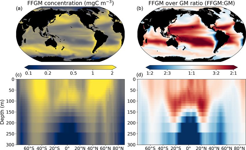
872                                                                   C. Clerc et al.: FFGM impacts on the ocean carbon cycle

Table 1. Variables and parameters used in the set of equations gov-   ity due to predation by unresolved higher trophic levels (with
erning the temporal evolution of the state variables                  a rate mX ) and mortality due to disease (with a rate mX      c ).
                                                                      All terms in this equation were given the same temperature
        Symbol      Description                                       sensitivity fX (T ) using a Q10 of 2.14 (Eqs. 25a and 25b in
                    I. State variables                                Aumont et al., 2015), as for mesozooplankton in PISCES-v2
                                                                      and according to Buitenhuis et al. (2006). Growth rate and
        P           Nanophytoplankton                                 quadratic mortality are reduced, and linear mortality is en-
        D           Diatoms                                           hanced at very low oxygen levels, as we assume that macro-
        Z           Microzooplankton
                                                                      zooplankton are not able to cope with anoxic waters (1(O2 )
        M           Mesozooplankton
        GM          GM
                                                                      varies between 0 in fully oxic conditions and 1 in fully anoxic
        FFGM        FFGM                                              conditions – see Eq. (57) in Aumont et al., 2015).
        CaFFGM      FFGM carcasses                                       The difference between the two macrozooplankton groups
        FpFFGM      FFGM fecal pellets                                lies in the description of the term GX , i.e., the ingested mat-
        CaGM        GM carcasses                                      ter. A full description of the equations describing GX is pro-
        FpGM        GM fecal pellets                                  vided in the Appendix A3 (Eqs. A1 to A12). Below, we
                                                                      present the two different choices of feeding representation
                    II. Physical variables
                                                                      that differentiate the dynamics of the two macrozooplankton
        T           Temperature                                       groups, GM and FFGM.
                    III. Growth                                          GM, namely generic macrozooplankton, is intended
                                                                      to represent non-tunicate macrozooplankton, such as eu-
        eX          Growth efficiency of X                            phausids, pteropods or large copepods. The parametrization
        aX          Unassimilation rate of X                          is similar to that of mesozooplankton (Eqs. 28 to 31 in
         X
        gm          Maximal X grazing rate
          X
                                                                      Aumont et al., 2015), and parameter values have been de-
        KG          Half-saturation constant for X grazing            rived using allometric scaling relationships (see Sect. 2.2.1).
        pYX         X preference for group Y
          X
                                                                      Therefore, in addition to conventional suspension feeding
        Ythresh     Group Y threshold for X                           based on a Michaelis–Menten parameterization with no
          X
        Fthresh     Feeding threshold for X                           switching and a threshold (Eqs. A1, A2 and A3), flux feed-
        wX          Sinking velocity of X particles
                                                                      ing is also represented (Eqs. A4), as has been frequently
        f fmX       X flux-feeding rate
                                                                      observed for both meso- and macrozooplankton (Jackson,
        mX          X quadratic mortality
                                                                      1993; Stukel et al., 2019). GM can flux feed on small and
        mXc         X non-predatory quadratic mortality
                                                                      large particles, as well as on carcasses and fecal pellets pro-
        rX          X linear mortality
        Km          Half-saturation constant for mortality
                                                                      duced by both GM and FFGM (Eq. A6). We assume that the
        α           Remineralization rate                             proportion of flux feeders is proportional to the ratio of po-
                                                                      tential food available for flux feeding to the total available
                                                                      potential food (Eqs. A7 and A8). Suspension feeding is sup-
                                                                      posed to be controlled solely by prey size, which is assumed
on the modeling choices differentiating these two groups. All
                                                                      to be about 1 to 2 orders of magnitude smaller than that of
symbols and definitions are summarized in Table 1.
                                                                      their predators (Fenchel, 1988; Hansen et al., 1994). Thus,
  The temporal evolution of the two compartments of
                                                                      GM preferentially feed on mesozooplankton but also, to a
macrozooplankton is governed by the following equation:
                                                                      lesser extent, on microzooplankton, large phytoplankton and
∂X                                                                    small particles (Eqs. A5 and A10, Fig. 1).
   = eX GX (1 − 1 (O2 )) fX (T )X                                        FFGM represent the large pelagic tunicates (i.e., salps, py-
∂t
   − (mX + mX                             2                           rosomes and doliolids but not appendicularians). Pelagic tu-
                c )fX (T ) (1 − 1(O2 )) X
                                                                    nicates are all highly efficient filter feeders and thus have ac-
                      X                                               cess to a wide range of prey sizes, from bacteria to meso-
   − r X fX (T )             + 31(O2 ) X.                      (1)
                   Km + X                                             zooplankton (Acuña, 2001; Sutherland et al., 2010; Bernard
                                                                      et al., 2012; Ambler et al., 2013). There is no strong evi-
  This equation is similar to the one used for micro- and             dence that FFGM feed on mesozooplankton in the literature.
mesozooplankton in PISCES-v2 (Aumont et al., 2015).                   Although there is some recent evidence for selective feed-
In this equation, X is the considered macrozooplankton                ing behavior in pelagic tunicates (Sutherland and Thomp-
biomass (GM or FFGM), and the three terms on the right-               son, 2022), the lack of quantitative study led to the simpler
hand side represent growth, quadratic and linear mortalities.         representation of FFGM as non-selective feeders (Pakhomov
eX is the growth efficiency. It includes a dependence on food         et al., 2002; Vargas and Madin, 2004; von Harbou et al.,
quality, as presented in PISCES-v2 (Eqs. 27a and 27b in Au-           2011). Therefore, we assume in our model that FFGM are
mont et al., 2015). Quadratic mortality is divided into mortal-       solely suspension feeders (i.e., with concentration-dependent

Biogeosciences, 20, 869–895, 2023                                                          https://doi.org/10.5194/bg-20-869-2023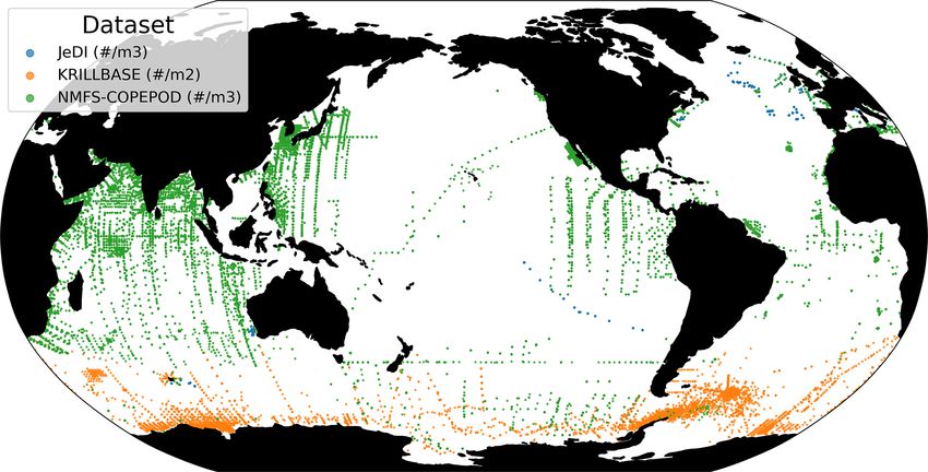
C. Clerc et al.: FFGM impacts on the ocean carbon cycle                                                                         873

grazing based on a Michaelis–Menten parameterization with
no switching and a threshold; see Eqs. A1, A2 and A3), feed-
ing with identical preferences on both phytoplankton groups
(D and N), as well as on microzooplankton (Z; Eqs. A11 and
A12, Fig. 1). They can also feed on small particles (sPOC;
Sutherland et al., 2010; Eq. A11, Fig. 1).

2.1.3    Carcasses and fecal-pellet dynamics

Carcasses CaFFGM and CaGM are produced as a result of non-       Figure 2. Histogram of the preferences of secondary consumers for
predatory quadratic and linear mortalities of GM and FFGM,       their respective prey. Secondary consumers are mesozooplankton,
respectively. The FpFFGM and FpGM are produced as a fixed        FFGM and GM, and prey are nanophytoplankton, diatoms, micro-
fraction of the total food ingested by the two macrozoo-         zooplankton, mesozooplankton, small organic particles and large
                                                                 organic particles. A preference of 1 indicates that any prey reached
plankton groups. Remineralization of fecal pellets and car-
                                                                 is consumed, and a preference of 0 indicates that the prey is never
casses by bacteria is modeled using the same temperature-        consumed.
dependent specific degradation rate with a Q10 of 1.9, iden-
tical to that used for small and large particles. In addition
to remineralization, carcasses and fecal pellets undergo flux    800 m d−1 (resp. 1000 m d−1 ; Henschke et al., 2016). The
feeding by GM as explained in the previous subsection. Note      sinking speeds of GM fecal pellets and carcasses are set
that parasitism is not considered in this study because it is    rather arbitrarily to 100 and 300 m d−1 respectively, within
too poorly documented, but it could represent an important       the wide range of values found in the literature (Small et al.,
source of carcasses (Lavaniegos and Ohman, 1998; Phleger         1979; Fowler and Knauer, 1986; Lebrato et al., 2013; Turner,
et al., 2000; Hereu et al., 2020). The sinking speeds of these   2015). The quadratic mortality rates have been adjusted by
particle pools are assumed to be constant. A complete de-        successive simulations evaluated against the observations
scription of the equations governing the temporal evolution      presented in the next section.
of fecal pellets and carcasses is provided in the Appendix A3
(Eqs. A14 and A15).                                              2.2.2    Reference simulation

2.2     Standard experiment                                      The biogeochemical model is run in an offline mode with
                                                                 dynamical fields identical to those used in Aumont et al.
2.2.1    Model parameters                                        (2015). These climatological dynamic fields (as well as the
                                                                 input files) can be obtained from the NEMO website (https:
Each zooplankton group is characterized by a size range, as-     //www.nemo-ocean.eu, last access: 17 November 2022) and
suming that sizes within the group are distributed along a       were produced using an ORCA2-LIM configuration (Madec,
spectrum of constant slope −3 in log–log space, according to     2008). The spatial resolution is about 2◦ by 2◦ cos(φ) (where
the hypothesis of Sheldon et al. (1972). These ranges are as     φ is the latitude) with a meridional resolution enhanced at
follows: 10–200 µm for microzooplankton, 200–2000 µm for         0.5◦ in the Equator region. The model has 30 vertical lay-
mesozooplankton and 2000–20000 µm for macrozooplank-             ers with increased vertical thickness, from 10 m at the sur-
ton (GM and FFGM).                                               face to 500 m at 5000 m. PISCES-FFGM was initialized from
   All parameters in PISCES-FFGM have identical values to        the quasi-steady-state simulation presented in Aumont et al.
those in Aumont et al. (2015). The only exception is the         (2015). The two macrozooplankton groups, their fecal pel-
mesozooplankton quadratic mortality rate, whose value has        lets and their carcasses were set to a small uniform value
been greatly reduced from its standard value of 3 × 10⁴ to       of 10−9 mol C L−1 . The model was then integrated for the
4×10³ L mol−1 d−1 , since predation by higher trophic levels     equivalent of 600 years, forced with 5 d averaged ocean dy-
is now explicitly represented.                                   namic fields and with a 3 h integration time step.
   The parameter values that were introduced in PISCES-
FFGM to represent the evolution of GM and FFGM are               2.3     Sensitivity experiments
given in Table 2. Metabolic rates are assumed to vary with
size according to the allometric relationship proposed by        Five sensitivity experiments were carried out to assess the
Hansen et al. (1997). Therefore, maximum grazing, respira-       sensitivity of the model to the chosen parameterization.
tion and flux-feeding rates were calculated from their val-         The first experiment, PISCES-GM (“generic macrozoo-
ues for mesozooplankton using a size ratio of 10. The prefer-    plankton”), was designed to investigate the impact of an ex-
ences of GM and FFGM for their different prey are detailed       plicit FFGM representation (with a different grazing param-
in Sect. 2.1.2. Their values are shown in Fig. 2. The sink-      eterization than GM) on the spatial and vertical distribution
ing speed of FFGM carcasses (resp. fecal pellets) is set to      of POC fluxes. In PISCES-GM, the FFGM ingestion rate

https://doi.org/10.5194/bg-20-869-2023                                                      Biogeosciences, 20, 869–895, 2023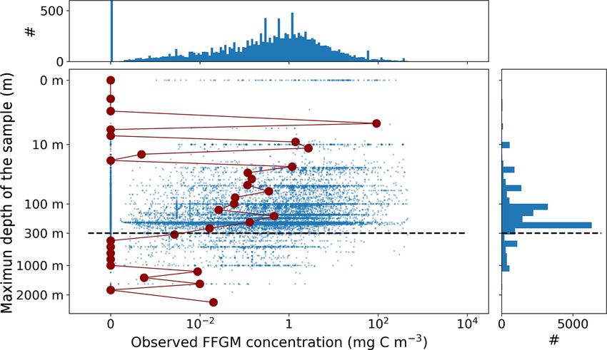
874                                                                   C. Clerc et al.: FFGM impacts on the ocean carbon cycle

Table 2. Parameter values used in PISCES-FFGM. The symbols in the “Source” column indicate how the parameter value was determined:
(?) indicates parameters for which we assumed that both GM and FFGM share the same characteristics as mesozooplankton; (•) indicates
metabolic rates assumed to vary with size, thus scaled using an allometric scaling conversion of mesozooplankton value based on (Hansen
et al., 1997); (†) indicates parameters tuned to fit PISCES-v2 general biology dynamics; and (‡) indicates parameters whose values have
been arbitrarily set based on information available in the literature and/or from the authors expertise.

                            Symbol        Source   GM (X = GM)        FFGM (X = FFGM)          Unit
                             X
                            emax            ?                 0.35                    0.35     –
                            aX              ?                   0.3                    0.3     –
                            gmX             •                 0.28                    0.28     d−1
                            KGX             ?            2 × 10⁻⁵               2 × 10⁻⁵       mol L−1
                            pXP             ‡                     0                   0.55     –
                            pXD             ‡                   0.3                   0.55     –
                            pXZ             ‡                   0.3                   0.55     –
                            pXM             ‡                     1                      0     –
                            pXPOC           ‡                   0.1                    0.4     –
                            pXGOC           ‡                   0.3                      0     –
                              X
                            Pthresh         ?                10−8                   10−8       mol L−1
                              X
                            Dthresh         ?                10−8                   10−8       mol L−1
                              X
                            Zthresh         ?                10−8                   10−8       mol L−1
                               X
                            Mthresh         ?                10−8                   10−8       mol L−1
                            POCX thresh     ?                10−8                   10−8       mol L−1
                              X
                            Fthresh         ?            3 × 10⁻⁷               3 × 10⁻⁷       mol L−1
                            wCaX            ‡                  300                    800      m d−1
                            wFpX            ‡                  100                   1000      m d−1
                            ffH
                              m             •              5 × 10⁵                       –     m2 mol−1
                                                                                                        −
                            mX              †            1.2 × 10⁴              1.2 × 10⁴      L mol−1 d 1
                            mXc             †              4 × 10³                4 × 10³      L mol−1 d−1
                            rX              •                0.003                  0.005      d−1
                            Km              ?            2 × 10⁻⁷               2 × 10⁻⁷       mol L−1
                            α               ?                0.025                  0.025      d−1

  FFGM defined in Table 1 and used in Eq. A3) was set to
(gm                                                                   speeds of particles from GM and FFGM. In PISCES-LOWV,
0, which is equivalent to running the model with a single             the sinking speeds of all fecal pellets and carcasses produced
generic macrozooplankton group.                                       by GM and FFGM (wFpX and wCaX , defined in Table 1 and
   The second experiment, PISCES-HGR (“high growth                    used in Eqs. A14 and A15) were assigned the same values as
rate”), was designed to investigate the impact of the higher          for large particles in PISCES-v2, i.e., 30 m d−1 .
clearance rates observed for FFGM than for GM. In PISCES-                The fifth experiment, PISCES-CLG (“clogging”), was de-
HGR, the FFGM ingestion rate (gm     FFGM defined in Table 1          signed to explore the impacts of clogging. Clogging, de-
and used in Eq. A3) was set to 1.4 d−1 , which corresponds            fined as the saturation of an organism’s filtering appara-
to a high value of the range provided by Luo et al. (2022)            tus with high levels of particulate matter, is a poorly docu-
(0.105–1.85 d−1 ).                                                    mented mechanism for FFGM but has been observed (Har-
   The third experiment, PISCES-HGM (“high growth and                 bison et al., 1986; Perissinotto and Pakhomov, 1997) or
mortality rates”), is similar to PISCES-HGR but tries to              suggested (Perissinotto and Pakhomov, 1998; Pakhomov,
compensate for the unrealistic high biomasses induced by              2004; Kawaguchi et al., 2004) for some salp species. Un-
FFGM high clearance rates in PISCES-HGR. To do so, non-               like other macrozooplankton groups, it has been shown that
predatory (mc ) quadratic mortality was increased so that             salp biomass remains relatively low at high chlorophyll con-
FFGM biomass on the upper 100 m is similar to PISCES-                 centrations (Heneghan et al., 2020). In PISCES-CLG, the
FFGM. The quadratic mortality due to predation was not                achieved ingestion rate of FFGM (GFFGM ; see Eq. A13) is
modified because there is no reason to believe that FFGM              modulated by a clogging function FC (Chl) inspired by the
are subject to a higher predation pressure than GM.                   parameterization proposed by Zeldis et al. (1995):
   The fourth experiment, PISCES-LOWV (“low velocity”),
was designed to evaluate the impact of the high sinking                                1
                                                                      FC (Chl) = 1 −     (1 + ERF (Csh (NCHL + DCHL − Cth ))) .    (2)
                                                                                       2

Biogeosciences, 20, 869–895, 2023                                                            https://doi.org/10.5194/bg-20-869-2023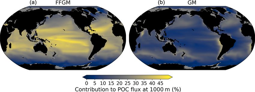
C. Clerc et al.: FFGM impacts on the ocean carbon cycle                                                                       875

In this equation, Cth is the clogging threshold, Csh is the       based on the maximum sampling depth of the corresponding
clogging sharpness, and ERF is the Gauss error function. A        net tows. In KRILLBASE, 5186 observations of thaliaceans
low clogging threshold Cth of 0.5 mg Chl m−3 is chosen to         with missing density values were discarded (35.6 % of the
limit FFGM growth in all moderate- and high-productivity          original 14 543 observations). In COPEPOD, concentrations
regions. Clogging sharpness Csh is set to 5 mg Chl m−3 , the      are standardized as if they were all taken from a plankton net
value proposed by Zeldis et al. (1995).                           equipped with a 330 µ m mesh (Moriarty and O’Brien, 2013).
   Values of the parameters that were changed in the five sen-    A total of 862 point observations with missing concentration
sitivity experiments are presented in Table 3. All five sensi-    values were discarded (3.5 % of the original 24 316 obser-
tivity experiments were initialized with the year 500 output      vations). We examined the composition of the original data
fields from the baseline PISCES-FFGM experiment. They             sources compiled within JeDI and COPEPOD by assessing
were then run for 100 years. All results presented in this        the recorded institution codes and their corresponding spatio-
study are values averaged over the last 20 years of each simu-    temporal distributions to evaluate the observations overlap-
lation. PISCES-CLG, PISCES-HGR and PISCES-HGM help                ping between these two previous data syntheses. We logically
to investigate the modeled distribution of GM and FFGM,           observed a very high overlap between COPEPOD and JeDI,
while PISCES-GM and PISCES-LOWV are used for explor-              as the former dataset was the main data contributor to the lat-
ing the spatial pattern and depth gradient of particulate or-     ter. Therefore, overlapping records were identified based on
ganic carbon fluxes.                                              their sampling metadata, scientific names, concentration val-
                                                                  ues, the recorded institution codes and recorded data sources,
2.4     Observations                                              and they were removed from JeDI. This removed 14 198
                                                                  (74.1 %) of the JeDI’s original thaliacean observations.
2.4.1    FFGM biomass estimates                                      This synthesis of thaliacean concentrations gathered glob-
                                                                  ally distributed 34 566 point observations (Fig. A1), col-
We compiled an exhaustive dataset of in situ pelagic tunicate     lected at a mean (± SD) maximum sampling depth of 193
(i.e., thaliacean) concentrations from large-scale plankton-      (± 198) m over the 1926–2009 time period (mean ± SD
monitoring programs and previous plankton data compila-           of the sampling year is 1975.9 ± 19.3). The range of ob-
tions to derive monthly fields of pelagic tunicates biomass (in   served thaliacean concentrations ranged from 0.0 ind m−3 to
mg C m−3 ). This product can be used as a standard dataset to     10 90 ind m−3 , with an average of 4.2 (± 103) ind m−3 .
evaluate the FFGM biomass estimated by PISCES-FFGM.                  Most of the records showed a fairly precise taxonomic res-
First, three main data sources were retrieved: NOAA’s             olution, as 1.6 % of the data were species resolved (mostly S.
Coastal and Oceanic Plankton Ecology, Production, and Ob-         thompsoni, Soestia zonaria, S. fusiformis and Thalia demo-
servation Database (COPEPOD; O’Brien, 2014); the Jel-             cratica), 42 % of the data were genus resolved (mostly
lyfish Database Initiative (JeDI; Lucas et al., 2014); and        Thalia, Doliolum and Salpa), and 83 % of the data were
KRILLBASE (Atkinson et al., 2017). The Australian Con-            family resolved (mostly Salpidae and Doliolidae). There-
tinuous Plankton Recorder (CPR) survey (AusCPR; IMOS,             fore, we were able to perform taxon-specific conversions
2021) and the Southern Ocean CPR survey (SO-CPR; Hosie,           from individual concentrations to biomass concentrations (in
2021) were excluded because they were found to not quan-          mg C m−3 ) for each point observation (see Table A1). We
titatively sample thaliaceans (see Appendix Text A1). This        used the taxon-specific carbon weights (mg C ind−1 ) summa-
compilation gathered planetary-scale plankton concentration       rized by Lucas et al. (2014), which were based on the group-
measurements collected through a broad variety of sampling        specific length–mass or mass–mass linear- and logistic-
devices over the last 100 years, with taxonomic identifica-       regression equations of Lucas et al. (2011). Not all the ob-
tion of varying precision and scientific names, some of which     servations had a precise counterpart in the carbon weights
changed through time. Therefore, we curated the scientific        compilation of Lucas et al. (2014) because they were not
names and the taxonomic classification of each observation        identified at the species or the genus level (e.g., class-level,
to harmonize names across all datasets and to correct dep-        order-level or family-level observations). In these cases, we
recated names and synonyms based on the backbone classi-          computed the median carbon weight of those taxa reported
fication of the World Register of Marine Species (WoRMS;          in Lucas et al. (2014) and which composed the higher-
WoRMS Editorial Board, 2023), using the “worms” R pack-           level taxonomic group (i.e., the carbon weight of Salpidae
age version 0.2.2 (Holstein, 2018). Then, only those obser-       corresponded to the average carbon weight of all Salpidae
vations corresponding to an organism belonging to the class       species), and we used this average carbon weight to con-
Thaliacea were kept. Observations without a precise sam-          vert the individual concentrations to carbon concentrations.
pling date and at least one sampling depth indicator (usu-        Biomass observations larger than 2 times the standard devia-
ally maximum sampling depth, in meters) were discarded.           tion were considered as outliers and were excluded. Then, we
All datasets provided concentrations in ind m−3 , except for      only retained observations from the upper 300 m to exclude
KRILLBASE, which provided salp (mostly Salpa thomp-               deep-water samples and to focus on zooplankton communi-
soni) densities in ind m−2 , which we converted to ind m−3        ties that inhabit the epipelagic layer – this is because mea-

https://doi.org/10.5194/bg-20-869-2023                                                      Biogeosciences, 20, 869–895, 2023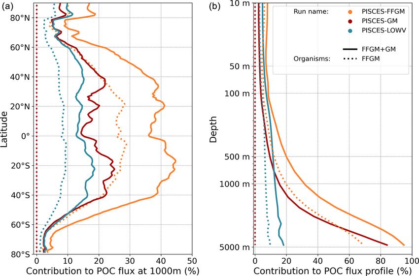
876                                                                                  C. Clerc et al.: FFGM impacts on the ocean carbon cycle

Table 3. Sensitivity experiments parameterization. A dash indicates that the parameter value is the same as in the standard PISCES-FFGM
experiment.

   Experiment                                       PISCES-FFGM (Standard)   PISCES-GM    PISCES-HGR   PISCES-HGM        PISCES-LOWV   PISCES-CLG
   FFGM maximal growth rate                         0.28 d−1                 0 d−1        1.4 d−1      1.4 d−1           –             –
   FFGM non-predatory quadratic mortality           4 × 10³ L mol−1 d−1      –            –            105 L mol−1 d−1   –             –
   Carcasses and Fecal pellets sinking velocities   100–1000 m d−1           –            –            –                 30 m d−1      –
   Clogging threshold                               ∞                        –            –            –                 –             0.5 mg Chl m−3

sured biomasses and sample numbers are low below 300 m                               with a mean size of 6.3 mm (the geometric mean of the
(see Fig. A2). The biomass levels of this subset ranged be-                          macrozooplankton size class) and applying the relationship
tween 0.0 and 488 mg C m−3 (4.9 ± 25.7 mg C m−3 ). Thali-                            proposed for copepods by Watkins et al. (2011).
acean concentrations issued from single-net samples were                                Monthly observation fields were binned on a 360 × 180
summed when necessary (e.g., when species and/or gen-                                grid to validate other modeled distributions. The mesozoo-
era counts were sorted within one plankton sample) to be                             plankton field (mmol m−3 , vertically integrated between 0
representative of a Thaliacea-level point measurement. At                            and 300 m to ensure that most of the organisms present in
this point, the dataset contains 18 875 single observations of                       the epipelagic zone are included) from MARine Ecosystem
thaliacean biomass. Hereafter, we will refer to this dataset as                      DATa (MAREDAT; Moriarty and O’Brien, 2013) is used to
“AtlantECO dataset”.                                                                 evaluate our modeled total mesozooplankton biomass distri-
   Ultimately, monthly thaliacean biomass fields were com-                           bution. The PO3−            −
                                                                                                     4 and NO3 surface fields from the World
puted for validating the monthly FFGM biomass fields of                              Ocean Atlas (Garcia et al., 2019) are used to evaluate our
PISCES-FFGM. Thaliacea biomass concentrations were av-                               modeled nutrient distributions. The long-term multi-sensor
eraged per month on a 72 × 36 grid to obtain the 12 monthly                          time series OC-CCI (Ocean Colour project of the ESA Cli-
climatological fields of Thaliacea biomass needed for eval-                          mate Change Initiative; Sathyendranath et al., 2019) of satel-
uating our model. Although some pelagic tunicate species                             lite phytoplankton chlorophyll a sea surface concentration
show a large extent of diel vertical migration (Pascual et al.,                      converted into mg Chl m−3 is used to evaluate our modeled
2017; Henschke et al., 2021b), the present observational                             total chlorophyll distribution. The same product regridded
data were averaged per month regardless of sampling time                             on a 72 × 36 grid is used to compare observed and mod-
due to the lack of precise quantitative information on the                           eled relationships between chlorophyll and FFGM abun-
taxon-specific magnitude and spatial heterogeneity of these                          dance (Fig. 5).
diel vertical migrations. Also, a low-resolution grid (5◦ × 5◦ )
has been used to counterbalance patchiness of data, as sug-                          2.4.3   Model evaluation
gested by Lilley et al. (2011). After this final step, the
monthly climatological values of Thaliacea biomass con-                              The model evaluation is based on monthly fields averaged
centrations ranged between 0.0 and 454 mg C m−3 (6.53 ±                              over the last 20 years of the PISCES-FFGM reference simu-
26.21 mg C m−3 ). Hereafter, we will refer to this climatology                       lation.
as “AtlantECO climatology”.                                                             For each unique observation in the AtlantECO dataset,
                                                                                     we sampled the modeled FFGM biomass from the PISCES-
2.4.2   Additional datasets                                                          FFGM climatology at the corresponding coordinates (lati-
                                                                                     tude, longitude), month and depth range (minimal depth and
We also used the monthly fields derived from observations                            maximal depth) so that each observed biomass can be com-
as a standard dataset to evaluate some of the other PISCES-                          pared to a “model-sampled” biomass. When compared to the
FFGM compartments: total macrozooplankton, mesozoo-                                  AtlantECO climatology, the annual mean FFGM biomass
plankton, total chlorophyll, nutrients and oxygen.                                   fields and the statistics (Table 4) are calculated from these
   As with FFGM, for total macrozooplankton observations,                            “model-sampled” biomasses to avoid bias due to sampling.
                                                                                                                                             3−
a low-resolution grid has been used. We use monthly macro-                              For other variables, model outputs (NO−       3 , PO4 , Chl,
zooplankton abundances binned on a 72 × 36 grid (ind m−3 ,                           mesozooplankton and GM+FFGM) were regridded horizon-
vertically integrated between 0 and 300 m to ensure that                             tally and vertically on the same grid as the corresponding
most of the organisms present in the epipelagic zone are in-                         observations (see previous section). The macrozooplankton
cluded) from MARine Ecosystem DATa (MAREDAT; Mo-                                     and mesozooplankton fields were integrated vertically on the
riarty et al., 2013) and then convert abundances to carbon-                          appropriate vertical range. When compared to observations,
based concentrations to evaluate our modeled distribution                            model outputs are sampled at exactly the same location and
of total macrozooplankton biomass (i.e., FFGM and GM).                               in the same month as the observations. Annually averaged
To convert to carbon concentration, an average individual                            fields, as well as statistics (Table 4), are computed from these
weight of 588 µg was chosen by considering an individual                             sampled fields to avoid bias due to sampling.

Biogeosciences, 20, 869–895, 2023                                                                        https://doi.org/10.5194/bg-20-869-2023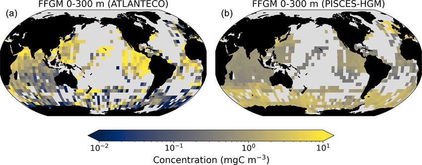
C. Clerc et al.: FFGM impacts on the ocean carbon cycle 877
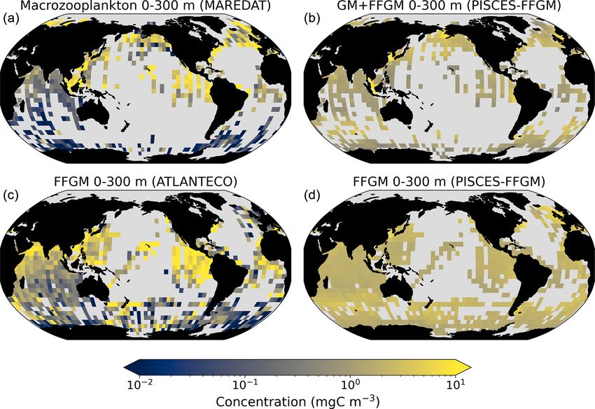
Figure 3. FFGM and FFGM : GM ratio. Annual mean of FFGM
carbon concentrations (mg C m−3 , log scale) averaged over the top
300 m (a) and zonally averaged (c). Annual of mean FFGM : GM Figure 4. Comparison between observed and modeled macro-
ratio, averaged over the top 300 m (b) and zonally averaged (d). zooplankton biomasses. Annual means of carbon concentrations
Red tones indicate FFGM dominance, and blue tones indicate GM (mg C m−3 , log scale) averaged over the top 300 m on a 5◦ reso-
dominance. lution grid. (a) Macrozooplankton from MAREDAT; (b) “model-
sampled” total macrozooplankton (GM + FFGM); (c) FFGM from
AtlantECO climatology; (d) “model-sampled” FFGM. As de-
scribed in Sect. 2.4.3, modeled biomasses were sampled where ob-
3 Results servations were available.
3.1 Macrozooplankton biomass
the subtropical domain, where deep chlorophyll maxima are
3.1.1 Simulated biomass located.
We first analyze the simulated living compartments of 3.1.2 Comparison to observations
PISCES-FFGM. The total integrated biomass of all living
compartments simulated by PISCES-FFGM is 1.4 Pg C for Next, we focus on the evaluation of the new components
the upper 300 m of the global ocean. Primary producers ac- added in this version of PISCES, i.e., GM and FFGM. In
count for 51 % of this biomass. Total macrozooplankton ac- the appendices, we present an evaluation of nitrate, chloro-
counts for 12 % of the total biomass. Our model predicts phyll and mesozooplankton (see Text A2 and Fig. A3). For
that FFGM and GM contribute roughly equally to macrozoo- these tracers, note that the performance of PISCES-FFGM is
plankton biomass, each having a biomass of about 0.08 Pg C. similar to that of PISCES-v2 (Aumont et al., 2015).
Figure 3 displays the annual mean FFGM carbon concentra- The annual mean distributions of total macrozooplank-
tion and the FFGM-to-GM ratio averaged over the top 300 m ton (FFGM and GM) and FFGM only, averaged over the
of the ocean. It also shows the zonally averaged distribu- top 300 m of the ocean, are compared to available obser-
tion of this concentration and of this ratio. Simulated FFGM vations (Fig. 4). A quantitative statistical evaluation of the
concentration is high (> 1 mg C m−3 ) in the subpolar regions model performance for these two fields is presented in Ta-
and close to the Equator and low (< 1 mg C m−3 ) in the olig- ble 4. The Spearman correlation coefficient between ob-
otrophic gyres and at extreme latitudes. The most striking served and modeled total macrozooplankton biomasses is
feature is the reverse distribution of the ratio as compared to 0.26 (p value < 0.001). Regions of high macrozooplank-
the simulated absolute biomass of both GM and FFGM. The ton biomass are correctly simulated in the Northern Hemi-
ratio exceeds 2 in oligotrophic subtropical gyres, while it is sphere by our model: 94 % of the area in which ob-
minimal in the most productive regions. In eastern-boundary served concentrations are greater than 0.5 mg C m−3 cor-
upwelling systems, FFGM biomass can be more than 2 times respond to areas in which the simulated concentration is
lower than GM biomass. Vertically, the ratio is, on aver- greater than 0.5 mg C m−3 . On the other hand, observations
age, larger than 1 in the euphotic zone. Below the euphotic suggest moderate biomass in the Indian Ocean (between
zone, it sharply decreases as GM become dominant. In the 0.05 and 0.5 mg C m−3 ) and low biomass in the Southern
mesopelagic domain, flux feeding has been shown to be a Ocean (lower than 0.05 mg C m−3 ). These low and moder-
very efficient mode of predation (Jackson, 1993; Stukel et ate biomasses are not captured by our model, which simu-
al., 2019). Since FFGM are not able to practice this feeding lates values greater than 0.5 mg C m−3 in both areas: 98 %
mode, they are out-competed by GM. The FFGM : GM ratio of the area in which observed concentrations are lower than
is at its maximum in the lower part of the euphotic zone in 0.5 mg C m−3 correspond to areas in which modeled con-
https://doi.org/10.5194/bg-20-869-2023 Biogeosciences, 20, 869–895, 2023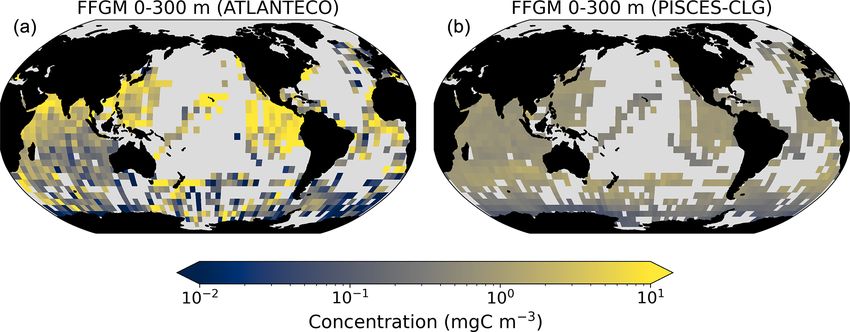
878                                                                     C. Clerc et al.: FFGM impacts on the ocean carbon cycle

Table 4. Macrozooplankton model vs. observation statistics. “Mean”, “median” and “standard deviation” are computed on all the non-zero
biomass values of the annual climatologies (as defined in Sect. 2.4.3) weighted by their respective cell areas. “Bias” is computed as the
difference between modeled and observed means. “Bias (log10)” is computed on log10-converted observed and modeled climatologies. “R
Spearman” is the Spearman correlation coefficient computed on non-zero values of the climatologies. “High biomasses match” is the percent-
age of observed area where biomasses greater than 0.5 mg C m−3 correspond to area where model biomasses are greater than 0.5 mg C m−3 .
“Low biomasses match” is the percentage of observed area where biomasses lower than 0.5 mg C m−3 correspond to area where model
biomasses are lower than 0.5 mg C m−3 . The cut-off value of 0.5 mg C m−3 , used for defining high- and low-biomass regions, corresponds
to the rounded median value of the macrozooplankton observations from MAREDAT (see Sect. 2.4.2).

                                      Total macrozooplankton           FFGM               FFGM                FFGM                 FFGM
               Experiment                     PISCES-FFGM       PISCES-FFGM          PISCES-CLG          PISCES-HGR          PISCES-HGM
 Model         Mean (mg C m−3 )                         1.65               1.18               0.69                 5.02                1.24
               Median (mg C m−3 )                       1.56               0.80               0.30                 4.59                0.98
               SD (mg C m−3 )                           1.29               0.96               0.69                 3.00                0.86
 Observation   Mean (mg C m−3 )                        11.01               8.22               8.22                 8.22                8.22
               Median (mg C m−3 )                       0.52               1.11               1.11                 1.11                1.11
               SD (mg C m−3 )                            128               26.9               26.9                 26.9                26.9
 Comparison    Bias (mg C m−3 )                        −9.36              −7.04              −7.53               −3.20                6.98
               Bias (log10)                             0.57               0.04              −0.18                0.60                0.02
               R Spearman                    0.26 (p < 10−5 )   0.17 (p < 10−5 )   0.34 (p < 10−5 )   −0.28 (p < 10−5 )   −0.22 (p < 10−5 )
               High biomasses match                    94 %               91 %               84 %                100 %                85 %
               Low biomasses match                      2 %               14 %               41 %                  0%                 18 %

centrations are greater than 0.5 mg C m−3 . Overall, the sim-
ulated distribution of macrozooplankton is too homogeneous
with respect to what the observations suggest. This is con-
firmed by the much smaller standard deviation in our model
simulation compared to that in the observations: 1.3 and
128 mg C m−3 respectively.
   Our model simulates a distribution of FFGM in the up-
per ocean that correlates with observations with a Spearman
correlation coefficient of 0.17 (p value < 0.001). The simu-
lated FFGM biomass is high (> 0.5 mg C m−3 ) in the equa-
torial domain of the Pacific and Atlantic oceans and in the
middle latitudes of both hemispheres. Conversely, FFGM
biomass is moderate (between 0.05 and 0.5 mg C m−3 ) in
the oligotrophic subtropical gyres and in the high lati-
tudes (> 60◦ ). Compared to observations, the spatial pat-
terns of high biomasses are better reproduced than for to-
tal macrozooplankton: 91 % of the area in which observed                Figure 5. Chlorophyll–FFGM relationship. Log–log scatter plot
concentrations are greater than 0.5 mg C m−3 correspond                 showing FFGM concentration versus total chlorophyll concentra-
to areas in which modeled concentrations are greater than               tion for PISCES-FFGM, PISCES-CLG clogging run, and the At-
0.5 mg C m−3 . However, the maximum observed values are                 lantECO vs. OC-CCI chlorophyll datasets. The datasets were grid-
strongly underestimated: the 95th percentile of the mod-                ded into an annual climatology with a spatial resolution of 5◦ . Each
eled values is 2.6 mg C m−3 , while it is 32 mg C m−3 in the            small dot corresponds to one grid cell of these climatologies. Large
observations. In the Southern Ocean, the simulated distri-              dots connected by a line represent the median per 0.07-wide log
bution is much more zonally homogeneous than that sug-                  bins of chlorophyll; dashed lines represent standard deviations be-
                                                                        low and above the median for each bin.
gested by observations (Fig. 4). Overall, the predicted me-
dian biomass of FFGM is similar to that of observations:
0.80 vs. 1.11 mg C m−3 . As with macrozooplankton, but to a
lesser extent, the simulated standard deviation is significantly           We also compared the observed and modeled relationships
lower than in the observations: 0.96 and 26.9 mg C m−3 re-              between FFGM biomass distributions and chlorophyll lev-
spectively. The standard and log10 biases are closer to 0 than          els. The dotted black lines and points in Fig. 5 show the
those calculated for macrozooplankton (Table 4).                        FFGM biomass from the AtlantECO database plotted against
                                                                        the corresponding chlorophyll concentrations from OC-CCI

Biogeosciences, 20, 869–895, 2023                                                              https://doi.org/10.5194/bg-20-869-2023
C. Clerc et al.: FFGM impacts on the ocean carbon cycle 879
(see Sect. 2.4.2). Despite considerable scatter, this data-
based analysis suggests a modest decrease of FFGM biomass
for chlorophyll concentrations above about 0.3 mg Chl m−3 .
Yet, this decrease is far from systematic, since even at high
chlorophyll concentrations, FFGM biomass can be very high
(> 10 mg C m−3 ). In our reference PISCES-FFGM simula-
tion (dotted blue line and points in Fig. 5), the median values
of FFGM biomass appear to be consistent with observations
at intermediate chlorophyll concentrations between 0.08 and
0.3 mg Chl m−3 . However, as already mentioned in the previ-
ous section, our model predicts a much weaker variability of
FFGM biomass. For higher chlorophyll concentrations, me-
dian FFGM levels become significantly larger than in the ob-
servations (up to 1 order of magnitude larger; see Fig. 5).
3.1.3 Sensitivity experiments
Here, we present the PISCES-HGR, PISCES-HGM and Figure 6. Schematic representation of carbon fluxes induced by pro-
PISCES-CLG sensitivity experiments and their influence on cesses related to FFGM. Values are in Pg C yr−1 . The upper part of
the FFGM modeled distributions. the diagram represents the sources and sinks of FFGM integrated
A 5-fold increase in the maximum growth rate in the globally over the first 100 m. The source is the grazing on the dif-
PISCES-HGR experiment leads to a 4-fold and 5-fold in- ferent prey. The arrow going from FFGM to FFGM corresponds to
the flux related to growth due to assimilated food. The sinks are as
crease in the mean and median FFGM concentrations, re-
follows: (i) the remineralization, non-assimilation and linear mor-
spectively (see Table 4). While the mean is closer to the tality that go into the dissolved organic carbon (DOC) and dissolved
observed mean than in the standard experiment, the nega- inorganic carbon (DIC); (ii) the quadratic predatory mortality term
tive Spearman coefficient shows the unrealistic nature of this (directly remineralized in PISCES-FFGM because of the lack of
simulation and the need to correct mortality accordingly (see explicit representation of upper-level predators); and (iii) the pro-
Table 4 and Fig. A4). The increase in mortality rate in the duction of particulate organic carbon (POC) via carcasses and fecal
PISCES-HGM experiment results in similar mean and me- pellets. The lower part of the diagram corresponds to the export of
dian FFGM biomass to that of the standard PISCES-FFGM POC linked to the fall of carcasses and fecal pellets of FFGM. The
experiment (see Table 4 and Fig. A5) but a worse data–model values in blue correspond to the global annual FFGM-driven POC
fit (see Table 4 and Fig. A7). Given the large range sug- flux through the corresponding depth, the values in parenthesis rep-
gested for the growth rate of FFGM (0.105–1.85 d−1 accord- resenting the total POC flux (i.e., related to FFGM, GM, bPOC and
sPOC).
ing to Luo et al., 2022), these results support the choice of a
conservative approach in our reference experiment (PISCES-
FFGM), where the FFGM maximal growth rate is identical
None of the sensitivity experiments reproduce the ob-
to that of GM (i.e., 0.28 d−1 ).
served spatial variability, which remains much higher than
The addition of clogging in PISCES-CLG increases the
the modeled spatial variability, similarly to the standard
model–data spatial correlation (Spearman’s correlation co-
experiment, and the distribution of observed biomasses is
efficient is 0.34 compared to 0.17 previously; see Table 4
consequently much more spread out than the model (see
and Fig. A7). This improvement is explained by a better
Fig. A7).
representation of areas with moderate and low biomass in
PISCES-CLG (concentrations < 0.5 mg m−3 ), especially in 3.2 Carbon cycle
the southern part of the Southern Ocean (see Fig. A6). In-
deed, 41 % of the areas where observations give values be- 3.2.1 Carbon export from the surface ocean
low 0.5 mg C m−3 correspond to areas where the model pre-
dicts values below 0.5 mg C m−3 (vs. only 14 % in PISCES- We first discuss the role of macrozooplankton in shaping the
FFGM). Also, as shown in Fig. 5, the addition of clogging carbon cycle in the upper ocean, focusing on differences be-
(dotted gold line and points) reduces the bias and thus re- tween GM- and FFGM-related surface processes. Table 5
produces the observed relationship between FFGM biomass shows the globally integrated sinking flux of organic car-
and chlorophyll a concentration better than the standard ex- bon particles at 100 and 1000 m, while Fig. 6 focuses on
periment. However, the simulated spatial variability remains the FFGM-driven carbon fluxes. The total export flux from
strongly underestimated (SD = 0.69 mg C m−3 in PISCES- the upper ocean (at 100 m) is 7.55 Pg C yr−1 (Table 5). This
CLG and 26.9 mg C m−3 in the AtlantECO climatology), and value is relatively similar to previous estimates using differ-
biases are increased when clogging is added (see Table 4). ent versions of PISCES (Aumont et al., 2015, 2017, 2018).
https://doi.org/10.5194/bg-20-869-2023 Biogeosciences, 20, 869–895, 2023880 C. Clerc et al.: FFGM impacts on the ocean carbon cycle
Table 5. Particulate carbon flux composition at 100 and 1000 m. Units are in Pg C yr−1 . sPOC (resp. bPOC) is for small (resp. large)
particulate organic carbon. CaGM (resp. CaFFGM ) is for GM (resp. FFGM) carcasses. FpGM (resp. FpFFGM ) is for GM (resp. FFGM) fecal
pellets.
Experiment Depth bPOC sPOC FpGM CaGM FpFFGM CaFFGM Total GM + FFGM FFGM
(m) (Pg C yr−1 ) (Pg C yr−1 ) (Pg C yr−1 ) (Pg C yr−1 ) (Pg C yr−1 ) (Pg C yr−1 ) (Pg C yr−1 ) contribution contribution
PISCES-FFGM 100 4.49 2.37 0.09 0.17 0.29 0.14 7.55 9% 6%
PISCES-GM 100 4.92 2.49 0.11 0.20 0.00 0.00 7.73 4% 0%
PISCES-LOWV 100 4.72 2.41 0.08 0.15 0.24 0.12 7.71 8% 5%
PISCES-FFGM 1000 1.18 0.12 0.11 0.14 0.27 0.15 1.97 34 % 21 %
PISCES-GM 1000 1.27 0.13 0.12 0.16 0.00 0.00 1.68 17 % 0%
PISCES-LOWV 1000 1.23 0.13 0.04 0.06 0.07 0.04 1.56 13 % 7%
It is also within the range of published estimates, i.e., 4– organic carbon at 100 m increases slightly to 7.71 Pg C yr−1 ,
12 Pg C yr−1 (e.g., Laws et al., 2000; Dunne et al., 2007; it is reduced by 20 % at 1000 m compared to the stan-
Henson et al., 2011; DeVries and Weber, 2017). Small and dard PISCES-FFGM run (1.56 Pg C yr−1 ; see Table 5). The
large particles produced by phytoplankton, microzooplank- macrozooplankton contribution is similar to that found in the
ton and mesozooplankton account for 91 % of this carbon standard model at 100 m (8 %), but the contribution is re-
flux. The remaining 9 % (0.69 Pg C yr−1 ; Table 5) is due duced to 13 % at 1000 m and to 20 % at 5000 m (Fig. 7). This
to macrozooplankton (FFGM+GM), with one third of this confirms that the strong contribution of macrozooplankton to
amount coming from carcasses and the remaining amount POC fluxes at depth in the standard run is explained by the
coming from fecal pellets. FFGM are responsible for an ex- very high sinking speeds of carcasses and fecal pellets. These
port of 0.43 Pg C yr−1 (Table 5), which represents 62 % of high sinking speeds prevent any significant remineralization
the total macrozooplankton contribution. of these particles as they sink to the seafloor.
The particularly large contribution from FFGM com- The PISCES-GM sensitivity experiment, in which FFGM
pared to GM comes from higher production (grazing of are not allowed to grow, shows a similar depth gradient of
0.94 Pg C yr−1 compared to 0.63 Pg C yr−1 for GM; Figs. 6 the macrozooplankton contribution (Fig. 7, red curve) com-
and S7), while both groups shows similar export efficiency. pared to the standard run but a lower contribution at each
A total of 45 % of the grazed matter is exported at 100 m, depth (by 10 %). Indeed, the transfer efficiency from 100
while the remaining 55 % is split between implicit predation to 1000 m differs by only 2 % between the two groups in
by upper trophic levels and loss to dissolved inorganic and the standard model (97 % for FFGM and 95 % for GM) so
organic carbon. that particles produced at the surface by both groups have a
similar fate towards the deep ocean. However, the estimated
3.2.2 Carbon transfer efficiency to the deep ocean transfer efficiency is biased, as both groups of organisms pro-
duce particles below 100 m. Because they can adopt a flux-
We then analyze how the representation of the two new feeding strategy of predation, GM occupy the whole water
macrozooplankton groups influences the fate of particulate column, whereas FFGM remain confined to the upper ocean
organic carbon in the deep ocean. At 1000 m, the total sim- (see Sect. 3.1 and Fig. 3). As a result, GM also produce par-
ulated POC flux is 1.97 Pg C yr−1 (Table 5). Thus, the flux ticles below 100 m, which contributes to the flux at 1000 m
transfer efficiency from 100 to 1000 m is 26 %. Most of this and explains the computed higher transfer efficiency. This is
strong flux reduction is due to the loss of small and large or- confirmed by the PISCES-LOWV experiment: the efficiency
ganic particles. Macrozooplankton-driven export is very ef- of FFGM is reduced to 30 % in this simulation, while that of
fective because it remains almost unchanged from 100 to GM is only reduced to 40 %, even though the carcass and fe-
1000 m – 0.69 and 0.67 Pg C yr−1 , respectively (Table 5). cal pellet sinking velocities of both groups are identical. As
Therefore, the contribution of macrozooplankton increases the remineralization processes are identical in the two runs,
strongly with depth to 34 % of the total carbon export at we can reasonably assume that the difference comes from the
1000 m (Fig. 7). The respective contribution of particles pro- relatively higher productivity below 100 m of GM compared
duced by GM and FFGM (carcasses and fecal pellets) to this to FFGM.
flux is almost identical at both depth horizons. At 5000 m,
more than 90 % of the carbon flux is due to macrozooplank-
3.2.3 POC flux spatial patterns
ton (Fig. 7).
The PISCES-LOWV sensitivity experiment, in which car-
cass and fecal pellet sinking speeds of both macrozooplank- Although the processes underlying the efficient sequestra-
ton groups are reduced to 30 m d−1 , shows a much greater at- tion of the particulate carbon issued from the two groups of
tenuation of POC fluxes with depth: while the total export of macrozooplankton are similar, we investigate how the spatial
Biogeosciences, 20, 869–895, 2023 https://doi.org/10.5194/bg-20-869-2023You can also read