Impacts of fertilization on grassland productivity and water quality across the European Alps under current and warming climate: insights from a ...
←
→
Page content transcription
If your browser does not render page correctly, please read the page content below

Biogeosciences, 18, 1917–1939, 2021
https://doi.org/10.5194/bg-18-1917-2021
© Author(s) 2021. This work is distributed under
the Creative Commons Attribution 4.0 License.

Impacts of fertilization on grassland productivity and water quality
across the European Alps under current and warming climate:
insights from a mechanistic model
Martina Botter1 , Matthias Zeeman2 , Paolo Burlando1 , and Simone Fatichi3
1 Institute
         of Environmental Engineering, ETH Zurich, Zurich, Switzerland
2 KarlsruheInstitute of Technology, Institute of Meteorology and Climate Research, Atmospheric Environmental Research,
Garmisch-Partenkirchen, Germany
3 Department of Civil and Environmental Engineering, National University of Singapore, Singapore

Correspondence: Martina Botter (botter@ifu.baug.ethz.ch)

Received: 29 July 2020 – Discussion started: 26 August 2020
Revised: 12 January 2021 – Accepted: 13 January 2021 – Published: 19 March 2021

Abstract. Alpine grasslands sustain local economy by pro-             The local soil hydrology has a crucial role in driving the
viding fodder for livestock. Intensive fertilization is common     NO− 3 use efficiency. The commonly applied fixed thresh-
to enhance their yields, thus creating negative externalities      old limit on fertilizer N input is suboptimal. We suggest
on water quality that are difficult to evaluate without reliable   that major hydrological and soil property differences across
estimates of nutrient fluxes. We apply a mechanistic ecosys-       sites should be considered in the delineation of best prac-
tem model, seamlessly integrating land-surface energy bal-         tices or regulations for management. Using distributed maps
ance, soil hydrology, vegetation dynamics, and soil biogeo-        informed with key soil and climatic attributes or systemat-
chemistry, aiming at assessing the grassland response to fer-      ically implementing integrated ecosystem models as shown
tilization. We simulate the major water, carbon, nutrient, and     here can contribute to achieving more sustainable practices.
energy fluxes of nine grassland plots across the broad Euro-
pean Alpine region. We provide an interdisciplinary model
evaluation by confirming its performance against observed
variables from different datasets. Subsequently, we apply the      1   Introduction
model to test the influence of fertilization practices on grass-
land yields and nitrate (NO− 3 ) losses through leaching under
                                                                   Alpine grasslands are a vital resource for the European econ-
both current and modified climate scenarios.                       omy. They provide a variety of ecosystem services such as
    Despite the generally low NO−   3 concentration in ground-
                                                                   maintaining biodiversity, protecting soil, and offering recre-
water recharge, the variability across sites is remarkable,        ational functions (Sala and Paruelo, 1997; Lamarque et al.,
which is mostly (but not exclusively) dictated by elevation.       2011; Schirpke et al., 2017). Above all, they sustain econ-
In high-Alpine sites, short growing seasons lead to less effi-     omy by providing fodder for livestock. To this purpose, high
cient nitrogen (N) uptake for biomass production. This com-        yields are desired, as they correspond to increasing income
bined with lower evapotranspiration rates results in higher        for farmers; hence, large amounts of fertilizers are applied
amounts of drainage and NO−    3 leaching to groundwater. Sce-
                                                                   every year. One of the most important components of fer-
narios with increased temperature lead to a longer growing         tilizers is nitrogen. On the one hand, nitrogen plays a cru-
season characterized by higher biomass production and, con-        cial role as a nutrient contributing to the grassland growth.
sequently, to a reduction of water leakage and N leaching.         On the other hand, it is one of the main responsible com-
While the intersite variability is maintained, climate change      ponents for environmental pollution from agriculture. Nitro-
impacts are stronger on sites at higher elevations.                gen is lost into the environment either through gaseous emis-
                                                                   sions of N2 O, N2 , and NH3 (Amon et al., 2006; Ibraim et al.,

Published by Copernicus Publications on behalf of the European Geosciences Union.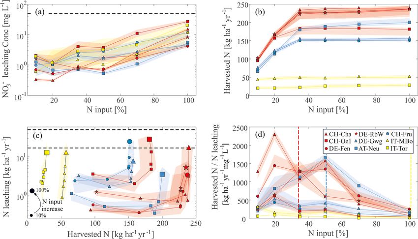
1918                                   M. Botter et al.: Impacts of fertilization and warming climate on Alpine grasslands

2019; Schlingmann et al., 2020) or as NO−     3 , either through   pose of supporting management, because they are thought to
surface runoff or as leaching to groundwater. Well-known           be difficult to operate, require a large amount of input data,
water quality issues, such as eutrophication, result directly      and require complex parameterization (see also discussions
from intensive management of grasslands (e.g., Heathwaite,         in Fatichi et al., 2019). However, when the above limita-
1995; Peukert et al., 2014). In order to tackle the problem of     tions are overcome, mechanistic models could provide in-
NO−  3 losses to the environment, the European Union (EU)          sights into biomass and nutrient budget quantification that
approved the Nitrate Directive 91/676/EEC (EEC, 1991),             would be too difficult to obtain otherwise. They can constrain
which imposes limits on the yearly load of fertilizers and re-     the description of soil biogeochemical processes by means of
stricts the fertilization season. In this frame, EU countries      mass and stoichiometric constraints better than empirical ap-
should pursue grassland management strategies designed             proaches, providing a larger predictive power (Moorhead et
with the intention of maximizing the grassland yields without      al., 1996; Wieder et al., 2013; Manzoni et al., 2016).
damaging the environment. The task is particularly daunt-             The NO−  3 leaching depends on the overall N cycle, which
ing given the spatial heterogeneity across the wide Alpine         results from the interplay of various processes. Hence, mech-
grassland areas and given the threat of climate change, which      anistic models reproducing the whole N cycle require a
is likely to remarkably impact the nitrogen cycle (Wang et         tight integration with models or modules dealing with land-
al., 2016). Elevation is often a major constraint for man-         surface exchanges of energy and water, vegetation dynamics,
agement in the Alpine environment, with low-elevation sites        soil hydrological and biogeochemical processes, and hydro-
generally being more prone to intensive management than            logical transport, in other words what are called ecosystem
high-elevation sites, for both climatological and pragmatic        or terrestrial biosphere models (Fatichi et al., 2016).
reasons. Since the EU Nitrate Directive has been in effect,           Different ecosystem models have been developed, but they
many studies attempted to quantify the NO−   3 fluxes with var-    rarely integrate all the abovementioned modules or treat them
ious methods (e.g., Kronvang et al., 2009; Groenendijk et al.,     with a similar level of complexity. For example, models that
2014). However, according to a questionnaire submitted to          were born as tools for the estimation of the greenhouse gas
grassland experts across EU countries, Norway, and Switzer-        emissions tend to simplify the soil hydrology using bucket-
land (Velthof et al., 2014), “non-academic” quantification of      type approaches. Some examples of this kind of models are
NO−  3 fluxes is still mainly based on expert estimates or on      CERES-EGC (Gabrielle et al., 1995; Gabrielle and Kengni,
prescribed values. Rarely models are applied. When they are,       1996; Hénault et al., 2005), DAYCENT (Parton et al., 1998,
the most common approach is the simple empirical feed bal-         2015; Del Grosso et al., 2000, 2002), STICS (Brisson et al.,
ance method, where grassland yields are estimated using sta-       1998, 2002, 2003), and DNDC (Li, 2000; Li et al., 2012),
tistical data on feed availability for ruminants and their feed    although efforts have recently been made to enhance the hy-
requirements. The nutrient balance is consequently estimated       drological module of the latter (Smith et al., 2020). In other
by applying values derived from literature or direct measure-      models, the soil hydrology module is represented with much
ments of nitrogen content in sampled grass.                        higher detail than the soil biogeochemistry module, as is the
   More complex modeling approaches for the quantifica-            case for HYDRUS-1D/2D/3D (Tafteh and Sepaskhah, 2012;
tion of nitrate losses from agricultural activity are emerging.    Phogat et al., 2013) or DAISY (Hansen et al., 1990; Hansen,
Some European projects have been promoted with the goal of         2002). More recently, ecosystem models were built by com-
assessing the state-of-the-art modeling tools in view of a har-    bining different models, each highly specialized in a spe-
monized assessment procedure across Europe. For example,           cific compartment of the ecosystem. The result leads to fully
the EUROHARP project (Kronvang et al., 2009) compares              integrated models such as ARMOSA (Perego et al., 2013),
available distributed models applied in different European         which is the combination SWAP (Van Dam, 2000) for the
countries. The analyzed models span from conceptual mod-           hydrological model, STAMINA (Ferrara et al., 2010; Richter
els such as NLES_CAT (Simmelsgaard and Djurhuus, 1998)             et al., 2010) for simulating the crop dynamics, and SOILN
and MONERIS (Behrendt et al., 2003) to more complex and            (Bergström et al., 1991) to represent the soil carbon and ni-
process-oriented models like SWAT and NL-CAT, which are            trogen cycles. The model SIM-STO (Pütz et al., 2018) was
born from the integration of ANIMO (Groenendijk et al.,            also created from the merging of SIMWASER (Stenitzer,
2005), SWAP (Kroes and Dam, 2003), SWQN (Smit et al.,              1988) and STOTRASIM (Feichtinger, 1998), which are fo-
2009), and SWQL (Siderius et al., 2008). Another example is        cused on water fluxes and nitrogen dynamics, respectively.
the GENESIS Project (Groenendijk et al., 2014), which com-         RT-Flux-PIHM (Bao et al., 2017) combines a reactive trans-
pares 1-D mechanistic models integrating hydrology, vegeta-        port (RT) model, a land-surface model (Noah LSM; Chen
tion dynamics, and soil biogeochemistry. The performance of        and Dudhia, 2001; Shi et al., 2013), and the hydrological
some models such as ARMOSA (Perego et al., 2013), Coup-            model PIHM (Shi et al., 2013). These models are usually
Model (Jansson, 2012), and EPIC (Williams et al., 1984; So-        performing well when applied with targeted applications. In
hier et al., 2009) are compared to simulated nitrate leaching      most of the cases they are validated only against the data
rates from lysimeters. What emerges from these studies is          concerning one specific module that is the most important to
that mechanistic models are currently not used for the pur-        solve the problem at hand. The models are hardly ever con-

Biogeosciences, 18, 1917–1939, 2021                                                  https://doi.org/10.5194/bg-18-1917-2021

M. Botter et al.: Impacts of fertilization and warming climate on Alpine grasslands                                          1919

currently evaluated against vegetation and soil water dynam-       (IT-MBo) in Italy; Oensingen (CH-Oe1), Chamau (CH-Cha),
ics or energy and biogeochemical fluxes. Here, we push the         and Früebüel (CH-Fru) in Switzerland; Neustift (AT-Neu) in
envelope of integrated models by applying the mechanistic          Austria; and Fendt (DE-Fen), Rottenbuch (DE-RbW), and
ecosystem model T&C-BG, which simulates the interactions           Graswang (DE-Gwg) in Germany. The mean annual precipi-
among vegetation dynamics, soil biogeochemistry, and hy-           tation (MAP) across sites ranges between 850 and 1627 mm,
drological fluxes. T&C-BG was recently developed (Fatichi          while mean annual temperature varies between 2.9 and 9.5
et al., 2019) as a single fully integrated model and there-        ◦ C following the elevation gradient (Table 1). All these sites

fore does not require many of the pragmatic simplifications        are permanent grassland ecosystems, mainly used for fodder
necessary to externally couple different models. We evaluate       production (Ammann et al., 2007; Hammerle et al., 2008;
the model capabilities by applying a “common” (non-site-           Vescovo and Gianelle, 2008; Kiese et al., 2018). Apart from
specific) parametrization to nine managed grassland sites          the site IT-Tor, which is unmanaged, the other grassland
across the broad Alpine region, derived from previous plot-        sites are managed with regular fertilizer applications and har-
scale studies (Fatichi et al., 2014; Fatichi and Pappas, 2017).    vested with grass cuts at standard height (0.07 m).
First, we evaluate the model against hydrological, energy,            Each site is equipped with a flux tower providing time se-
vegetation, and soil biogeochemical observations according         ries of micrometeorological variables, as well as energy (e.g.,
to the available data. Then, we run numerical experiments to       net radiation, latent heat, sensible heat) and carbon diox-
estimate the grass yields and the losses of NO−  3 under differ-   ide fluxes by means of the eddy covariance (EC) method
ent fertilization regimes and compare results across the sites.    (Aubinet et al., 2012). The flux tower data for all the sites
Ultimately, we simulate a climate change sensitivity test for      except the German ones are retrieved from the FLUXNET-
each management scenario by modifying atmospheric CO2              2015 database (Pastorello et al., 2020). German sites (DE-
concentrations by +250 ppm and air temperature by +3 ◦ C,          Fen, DE-RbW, DE-Gwg) belong to the Pre-Alpine Observa-
to compare results with outcomes from the simulations under        tory of the TERENO network (Zacharias et al., 2011; Pütz
present climate. Specifically, we investigate and answer the       et al., 2016; Kiese et al., 2018), where lysimeters are also
following questions:                                               installed in proximity to the flux tower site (Fu et al., 2017,
                                                                   2019; Zeeman et al., 2017; 2019).
    1. Is a mechanistic ecosystem model provided with a               For the stations DE-Fen, DE-RbW, and DE-Gwg, annual
       common parameterization for Alpine managed grass-           totals of lysimeter evapotranspiration (ET) and water leakage
       lands able to reliably represent the ecosystem dynamics     are retrieved for the years 2012–2014 from Fu et al. (2017,
       across nine sites?                                          2019). The same study provides annual DOC-C (dissolved
    2. How do grass productivity and leaching NO−                  organic carbon) and nitrate-N (N-NO−   3 ) concentrations in the
                                                     3 change
       in response to different fertilization scenarios and to     water leached at the bottom of the lysimeter. The ScaleX
       warming climate across the broad Alpine region?             campaign of 2015 (Wolf et al., 2017; Zeeman et al., 2019)
                                                                   provided additional data concerning harvested biomass and
    3. Can mechanistic models provide insights for legisla-        its carbon and N content.
       tors setting guidelines for management also in view of
       changing climatic conditions?                               2.2   T&C-BG model
Answering these questions, beyond allowing the assessment          We simulate the grassland ecosystem dynamics in each site
of a state-of-the-art ecosystem model in reproducing multi-        with the fully coupled terrestrial biosphere and ecosystem
ple aspects of ecosystem functioning, also provides quantita-      model T&C-BG, introduced by Fatichi et al. (2019), who
tive information that can be used to delineate best grassland      provided a complete model description. T&C-BG combines
management practices.                                              a well-tested ecohydrological model (T&C, e.g., Fatichi
                                                                   et al., 2012a, b, 2014, 2015; Manoli et al., 2018; Mas-
2     Study sites and methods                                      trotheodoros et al., 2020) with a soil biogeochemistry mod-
                                                                   ule, which represents soil carbon and nutrient dynamics as
2.1    Study sites and instrumentation                             well as plant mineral nutrition and multiple feedbacks be-
                                                                   tween nutrient availability, plant growth, and soil mineraliza-
The study sites are located in the European Alps and cover         tion processes. The T&C-BG model inputs include hourly lo-
an elevation gradient ranging between 393 and 2160 m a.s.l.        cal observations of microclimate (i.e., precipitation, air tem-
We used grassland sites in the Alpine region for which at          perature, wind speed, relative humidity, incoming shortwave
least eddy covariance flux tower observations were avail-          and longwave radiation, atmospheric pressure) and resolves
able. For a subset of sites, additional observations about         the principal land-surface energy exchanges (i.e., net radia-
leaf area index, soil moisture, grass productivity, and wa-        tion, sensible and latent heat), which are interconnected with
ter and nitrogen leaching were also available. Specifically,       hydrological processes, such as evaporation and transpira-
we used the sites of Torgnon (IT-Tor) and Monte Bondone            tion, infiltration, runoff, saturated and unsaturated zone water

https://doi.org/10.5194/bg-18-1917-2021                                                   Biogeosciences, 18, 1917–1939, 2021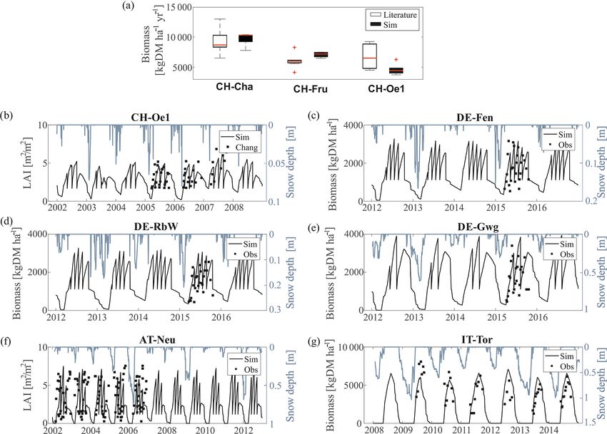
M. Botter et al.: Impacts of fertilization and warming climate on Alpine grasslands
https://doi.org/10.5194/bg-18-1917-2021
Table 1. Site characteristics. The following main site characteristics are reported: elevation, latitude, longitude, period for which measurements are available, mean annual precipitation
(MAP), mean air temperature (mean Ta ), number of grass cuts per year, and main references to original studies referring to the study sites. The values of MAP and mean Ta are computed
from the available time series.
Site Elevation Lati- Longi- Years of MAP Mean No. of Soil sand Dominant References
(m a.s.l.) tude tude available (mm) Ta cuts per and clay species
data (◦ C) year content
CH-Cha 393 47◦ 120 8◦ 240 2006–2014 1134 9.4 6 24 % clay Lolium multiflorum, Trifolium repens Gilgen and Buchmann (2009);
25 % sand Zeeman et al. (2010)
CH-Oe1 450 47◦ 170 7◦ 440 2002–2008 1222 9.2 3 20 % clay Lolium perenne, Alopecurus pratensis, Ammann et al. (2007, 2009)
60 % sand Trifolium repens
DE-Fen 600 47◦ 570 11◦ 060 2012–2016 850 7.8 5 30 % clay Lolium multiflorum Lam., Trifolium Kiese et al. (2018)
27 % sand repens L.
DE-RbW 770 47◦ 700 10◦ 980 2012–2016 955 7.4 5 29 % clay Lolium multiflorum Lam., Trifolium Kiese et al. (2018)
26 % sand repens L.
DE-Gwg 864 47◦ 570 11◦ 030 2012–2016 1114 5.3 2 52 % clay Lolium multiflorum Lam., Trifolium Kiese et al. (2018)
9 % sand repens L.
AT-Neu 970 47◦ 120 11◦ 320 2002–2012 856 6.8 3 11 % clay Dactylis glomerata, Festuca pratensis, Hammerle et al. (2008);
42 % sand Arrhenatherum elatius, Trifolium sp., Wohlfahrt et al. (2008a, 2010)
Taraxacum officinalis, Ranunculus
acris
CH-Fru 982 47◦ 600 8◦ 320 2005–2014 1627 7.6 4 22 % clay Alopecurus pratensis, Dactylis glom- Gilgen and Buchmann (2009);
29 % sand erata, Taraxacum officinalis, Ranuncu- Zeeman et al. (2010)
lus sp., Trifolium repens
Biogeosciences, 18, 1917–1939, 2021
IT-MBo 1550 46◦ 000 11◦ 020 2003–2013 1268 5.2 1 22 % clay Nardetum alpigenum Gilmanov et al. (2007);
29 % sand Vescovo and Gianelle (2008);
Gianelle et al. (2009); Marcolla
et al. (2011)
IT-Tor 2160 45◦ 500 7◦ 340 2008–2015 870 2.9 0 10 % clay Nardus stricta L., Festuca nigrescens Migliavacca et al. (2011);
45 % sand All., Arnica montana L. Galvagno et al. (2013);
Filippa et al. (2015)
1920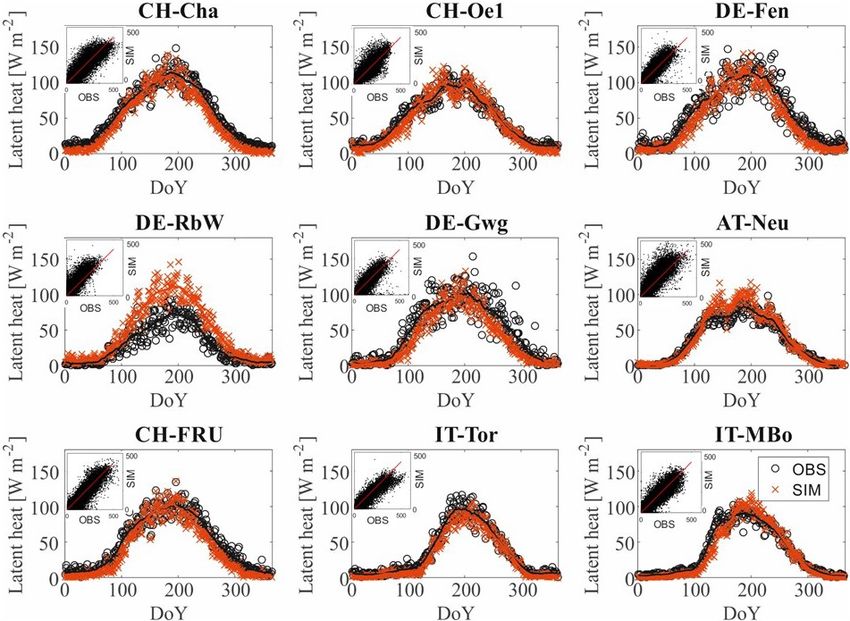
M. Botter et al.: Impacts of fertilization and warming climate on Alpine grasslands                                             1921

dynamics, groundwater recharge, and snow and ice hydrol-           1.4 m, corresponding to the depth of lysimeters, which is dis-
ogy dynamics. The soil hydrology module solves the 1-D             cretized into 16 soil layers of increasing depth from the sur-
Richard’s equation in the vertical direction and uses a heat       face to the bedrock. The biogeochemistry active zone is fixed
diffusion solution to compute the soil temperature profile. A      at 25 cm depth, and the grass roots are assumed to be expo-
soil-freezing module has also been recently introduced (Yu et      nentially distributed with a maximum rooting depth of also
al., 2020). The vegetation module computes photosynthesis,         25 cm. We do not simulate the groundwater dynamics, but
respiration, vegetation phenology, and carbon and nutrient         we compute the groundwater recharge as the water leakage
budgets including allocation to different plant compartments       at 1.40 m depth. The parameters selected for all simulations
and tissue turnover.                                               are detailed in Table S1 in the Supplement where the few
    The management of vegetation such as grass cuts and fer-       site-specific parameters are highlighted in bold.
tilization can be prescribed as part of model inputs. The soil         In each site we force the model with the local meteorolog-
biogeochemistry module accounts for the carbon and nutri-          ical conditions, while atmospheric CO2 concentrations are
ent budgets of litter and soil organic matter. Mineral nitro-      assumed to follow the observed historical global trend (Keel-
gen (N), phosphorous (P), and potassium (K) budgets and            ing et al., 2009). Nutrient depositions in the absence of local
the nutrient leaching are also simulated. This study is partic-    specific information for each site are set using global maps of
ularly focused on NO−   3 . Nitrate pool in the soil depends on    recently observed values for nitrogen and phosphorus (Gal-
the net immobilization and/or mineralization fluxes, nitrogen      loway et al., 2004; Mahowald et al., 2008; Vet et al., 2014).
uptake, nitrogen leaching, and nitrification and/or denitrifica-       Simulations corresponding to the described setup are used
tion fluxes, with the latter that are simulated with empirical     for evaluating the model performance before running the sce-
functions of the amount of NO−     3 and environmental condi-      nario analysis, and they represent the reference simulations.
tions (detailed description in Fatichi et al., 2019). The NO− 3    We evaluate the model performance against an ensemble of
transport process is not solved within the soil column, but        diverse variables. First, we compare simulated and observed
leaching is assumed to occur at the bottom of the soil col-        net radiation, latent heat, sensible heat, gross primary pro-
umn and is proportional to the water leakage and bulk NO−     3    duction (GPP), and net ecosystem exchange (NEE) using
concentration in soil water in the soil biogeochemical active      flux tower data. Second, we test the hydrological module
zone (Fatichi et al., 2019).                                       by comparing the effective soil saturation (e.g., normalized
    The model can be run in a distributed topographically          soil moisture) from the model and from local measurements.
complex domain (e.g., Mastrotheodoros et al., 2019, 2020),         Third, we evaluate the vegetation module comparing the sim-
but here it is employed in its plot-scale version, which simply    ulated biomass and/or leaf area index (LAI) dynamics with
solves 1-D vertical exchanges. In summary, based solely on         data retrieved from literature wherever available (Ammann
meteorological inputs, soil, and vegetation parameters, T&C-       et al., 2007; 2009; Hammerle et al., 2008; Gilgen and Buch-
BG simulates prognostically all the other variables, from en-      mann, 2009; Zeeman et al., 2010; Chang et al., 2013; Finger
ergy, carbon, and water fluxes via vegetation biomass up to        et al., 2013; Filippa et al., 2015; Prechsl et al., 2015). Finally,
soil nutrient mineralization and leaching. All these processes     we compare biogeochemical fluxes in terms of harvested ni-
interact with each other.                                          trogen and carbon, as well as leaching of NO−    3 and DOC. The
                                                                   evaluation of the soil biogeochemistry module is possible
2.3   Model parametrization                                        only for the sites DE-Fen, DE-RbW, and DE-Gwg (equipped
                                                                   with lysimeters); however, differences in scale, soil proper-
The model allows the simulation of different vegetation            ties, and timing of management between flux tower footprint
types, but in this case only grass is included. In order to        and lysimeters exist (Oberholzer et al., 2017; Mauder et al.,
keep results general enough and maximize future model              2018).
transferability across grassland sites, we adopt a common              Detailed manure input data for all the case studies were
parametrization for all of the nine sites with a few excep-        not available. To bypass this problem, whenever we did not
tions justified by elevation-dependent parameters such as          have information about fertilization (i.e., in all sites except in
threshold temperature for leaf onset. Vegetation parameter         the German ones), we assume that the cut grass is left on the
selection was based on previous experience with European           ground only for the reference simulations. Such a hypothesis
grasslands (Fatichi et al., 2014; Fatichi and Pappas, 2017);       is clearly unrealistic, because it opposes the purpose of the
soil biogeochemistry parameters are currently fixed for all        grassland management (i.e., producing yields), but it guaran-
sites in the absence of more specific information (see discus-     tees a nearly closed nutrient cycle, thus performing the same
sion in Fatichi et al., 2019). The site-specific soil content of   function of fertilizers, but providing the most targeted fer-
clay, sand, and organic matter in each site is provided as in-     tilization possible. While aiming at testing the model per-
put parameter to the model, which internally computes the          formance on the baseline scenario, such a hypothesis is pre-
hydraulic soil parameters by means of pedo-transfer func-          ferred to assuming a fertilization rate for each site to avoid
tions (Saxton and Rawls 2006). To make results compara-            excessive or insufficient nutrient addition.
ble, across all the sites, we assume a soil depth equal to

https://doi.org/10.5194/bg-18-1917-2021                                                    Biogeosciences, 18, 1917–1939, 2021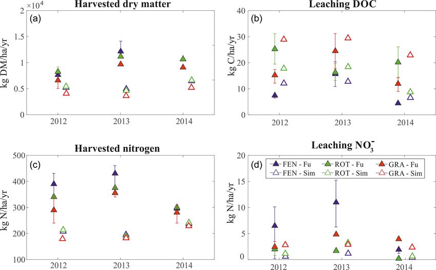
1922                                   M. Botter et al.: Impacts of fertilization and warming climate on Alpine grasslands

   In DE-Fen, DE-RbW, and DE-Gwg, the sites where both             500 kg ha−1 yr−1 (highly intensive management). This up-
the flux tower and the lysimeters are co-located, grassland        per limit intentionally exceeds the actual management prac-
is managed slightly differently above the lysimeters and in        tices and allows us to analyze what can happen if fertilization
the flux tower footprint. To validate model results, we ran        loads are increased. We computed the corresponding single
multiple simulations, each fed with the corresponding man-         application amount of manure based on C : N ratio of ma-
agement of either flux tower or lysimeter plots.                   nure equal to 8.9, which is reported for the sites of DE-Fen,
   Since the current initial conditions of the carbon and nutri-   DE-RbW, and DE-Gwg (Fu et al., 2017) and is also similar to
ent pools in the soil are unknown, as is common in modeling        values suggested in literature (Sommerfeldt et al., 1988; Nya-
studies, we spin up carbon and nutrient pools running only         mangara et al., 1999) or slightly lower (Zhu, 2007; Kumar et
the soil-biogeochemistry module for 1000 years using av-           al., 2010). The input of P and K is assumed to be propor-
erage climatic conditions with prescribed litter inputs taken      tional to the N input based on assigned N : P and N : K val-
from preliminary simulations with the soil-biogeochemistry         ues, guaranteeing non P- or K-limited conditions to the sys-
module inactive. Then we used the spun-up carbon and nutri-        tem. The specific manure amount computed for pre-Alpine
ent pools as initial conditions for the hourly scale fully cou-    sites is applied for Alpine and high-Alpine sites at the cor-
pled simulation over the period for which hourly observa-          responding lower frequencies. The resulting annual loads in
tions are available. This last operation is repeated two times,    all the scenarios are reported in Table 2. For each fertiliza-
which allows for reaching a dynamic equilibrium. We com-           tion scenario, in each site, we spin up the system running the
pare available observation of soil C : N values retrieved from     soil-biogeochemistry module for 1000 years under average
literature with the values resulting from such a spin-up pro-      climatic conditions and the specific management scenario.
cess.                                                              Thus, the initial conditions of each simulation correspond to
                                                                   the final state of the spin-up simulation run for each specific
2.4    Numerical fertilization experiments and climate             site and management scenario. Finally, we run each manage-
       change scenario                                             ment scenario in each site under both historical and modified
                                                                   climate scenario, representing the latter with an increase in
We set up numerical experiments to test the response of            atmospheric CO2 concentration of 250 ppm and an increase
the study sites to different manure application regimes un-        in air temperature of +3 ◦ C.
der historical climate and with modified temperature and              In the results analysis, we focus our attention on the re-
atmospheric CO2 conditions potentially representative of           sulting N contribution to grass productivity and on the N
the future. First, we classify the sites based on elevation        lost as leaching at the bottom of the soil profile. The for-
and management. We defined pre-Alpine/Intensive sites as           mer represents one of the positive gains from agriculture as
those located at elevations lower than 800 m a.s.l. and in-        economic activity and the latter a negative externality into
tensively managed (CH-Cha, CH-Oe1, DE-Fen, DE-RbW),                the environment, as most NO−   3 leaching will ultimately reach
Alpine/Extensive for sites with an altitude between 800 and        the groundwater storage and the rivers. We evaluate the dif-
1000 m a.s.l. and extensively managed (DE-Gwg, AT-Neu,             ferent management strategies by bringing together the two
CH-Fru), and high-Alpine/Extensive sites as those above            indicators in an index computed as the ratio of harvested N
1000 m a.s.l. and extensively managed, which include the           to N-NO−  3 leachate. The higher the value of the index, the
two grasslands of IT-MBo and IT-Tor. It is common prac-            most favorable is the management strategy for both farm-
tice among farmers to fertilize at the beginning of the grow-      ers and the environment. Thus, we interpret this index as a
ing season and after each cut. The numbers of cuts and ma-         proxy of the efficiency of the grassland in profiting from the
nure applications during the year decrease with elevation. Al-     N added in fertilization. We also analyze potential relations
though the time intervals between cuts can be similar, the         between such an efficiency index and site-specific character-
length of the winter dormant period ultimately determines          istics, such as the elevation and the percentage of precipita-
growing season length and, in turn, the number of cuts, the        tion that becomes groundwater recharge. We further assess
volume of locally needed organic fertilizer, and the opportu-      the impact of increased atmospheric CO2 concentration and
nity to bring that out into the field. We aligned the manage-      temperature on the short term by comparing the results of the
ment strategy of our numerical experiments to these notions        historic and modified climate scenarios. We compare vari-
and used a classification of the sites into three groups. In our   ables such as water leakage, harvested N, and N leaching,
simulations, manure is applied 6, 4, and 2 times, and the grass    and we analyze their implications for the efficiency index.
is cut 5, 3, and 1 times, respectively, in pre-Alpine, Alpine,
and high-Alpine sites. Grass is cut at a height of 0.07 m, fol-
lowing common practice. Referring to literature (Ammann
et al., 2007, 2012; Merbold et al., 2014; Fu et al., 2017), we
identified a broad range of possible N yearly loads applied in
grasslands. For pre-Alpine sites, the simulated range spans
between 50 kg ha−1 yr−1 (i.e., extensive management) and

Biogeosciences, 18, 1917–1939, 2021                                                  https://doi.org/10.5194/bg-18-1917-2021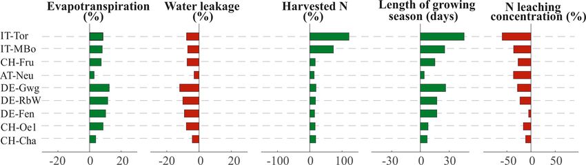
M. Botter et al.: Impacts of fertilization and warming climate on Alpine grasslands                                                      1923

Table 2. Numerical experiments. The sites are divided into pre-Alpine, Alpine, and high-Alpine sites based on the elevation in which they
are located. For each class, the numbers of cuts and manure applications as well as the yearly N load injected in the different modeling
experiments are reported. The specific manure application is the same for each site class, but the total amount varies across classes as the
number of yearly applications is different. The results are presented as a function of the percentage of max N input, reported in the table for
each experimental setup.

      Pre-Alpine/Intensive         Alpine/Extensive              High-Alpine/Extensive
      CH-Cha, CH-Oe1,              DE-Gwg, AT-Neu,               IT-MBo, IT-Tor
      DE-Fen, DE-RbW               CH-Fru
      5 cuts, 6 fertilizations     3 cuts, 4 fertilizations      1 cut, 2 fertilizations
      Yearly N load                Yearly N load                 Yearly N load               Specific manure     Percent of max N input
      (kg N ha−1 yr−1 )            (kg N ha−1 yr−1 )             (kg N ha−1 yr−1 )           application
                                                                                             (kg C ha−1 yr−1 )
      50                           33                            17                          74                  10 %
      100                          67                            33                          148                 20 %
      175                          117                           58                          260                 35 %
      250                          167                           83                          371                 50 %
      350                          233                           117                         519                 70 %
      500                          333                           167                         742                 100 %

Table 3. Coefficient of determination (R 2 ) of the simulated vs. ob-           We show the comparison between the observed and the
served energy and carbon fluxes from flux tower data.                        simulated effective saturation of the soil (Fig. 3) to evaluate
                                                                             the hydrological dynamics. The intra-annual pattern is gen-
                            Net    Sensible    Latent     GPP                erally well captured by the model. The average coefficient
                       radiation       heat      heat                        of determination R 2 equals 0.49, and the average RMSE is
                                                                             0.10. Results highlight the pedo-climatic differences across
         CH-Cha             0.98       0.63      0.86     0.78
         CH-Oe1             0.98       0.66      0.82     0.69               the Alpine region. Some sites tend to reach field capacity
         DE-Fen             0.97       0.51      0.79     0.66               quite easily (e.g., DE-Fen, DE-RbW, and DE-Gwg); in other
         DE-RbW             0.74       0.48      0.76     0.63               sites effective saturation is often below 50 % (CH-Cha, CH-
         DE-Gwg             0.74       0.39      0.70     0.59               Oe1, AT-Neu, and CH-Fru). The high-Alpine sites IT-Tor and
         AT-Neu             0.95       0.53      0.85     0.83               IT-MBo fall into this second case but with pronounced peaks
         CH-Fru             0.96       0.72      0.87     0.85               of saturation when snowmelt occurs.
         IT-MBo             0.93       0.75      0.88     0.79                  A summary of the simulated site-specific variables in
         IT-Tor             0.94       0.69      0.87     0.72               terms of water, energy, and carbon fluxes is shown in Ta-
                                                                             ble 4. The total net radiation does not vary consistently with
                                                                             elevation. As a result of temperature constraints, latent heat
3     Results                                                                decreases with increasing elevation, leading to lower ET in
                                                                             high-Alpine sites, as the higher values of the Bowen ratio for
3.1    Model evaluation                                                      the high-Alpine sites indicates. Phenology is also affected by
                                                                             elevation, and the average day of the year when the simu-
The performance of the model in representing the energy and                  lated growing season starts (taken as the mean day when the
carbon fluxes measured from the flux towers is good across                   biomass is higher than the biomass threshold at cut height)
all the sites. The R 2 values of the model and observations                  increases with increasing elevation. It spans from mid-March
comparison are reported in Table 3, and further goodness                     in the pre-Alpine site CH-Cha to mid-May in the high-Alpine
of fit metrics are reported in Table S2 in the Supplement.                   sites of IT-MBo and IT-Tor. Consequently, the mean yearly
The seasonality of the energy and carbon fluxes is well rep-                 GPP is higher when the growing season starts earlier. For in-
resented across all the study sites, as illustrated by the pattern           stance, the resulting mean annual GPP in CH-Cha is more
of latent heat shown in Fig. 2 and the patterns of sensible heat             than double compared to IT-Tor. However, the average GPP
H , GPP, and NEE reported in Figs. S1, S2, and S3 in the Sup-                of the month July only, intended as a proxy for the GPP in
plement, respectively. One exception is the NEE seasonality                  the maximum growth period, does not differ much across the
in sites where top soil freezing is simulated as IT-MBo, with                sites, and lower values are rather indicative of water limita-
NEE peaking later in the model.                                              tions, testifying to similar levels of productivity in the peak
                                                                             of the summer regardless of the site elevation.

https://doi.org/10.5194/bg-18-1917-2021                                                             Biogeosciences, 18, 1917–1939, 2021
1924                                     M. Botter et al.: Impacts of fertilization and warming climate on Alpine grasslands

Figure 1. Location of the study sites. The nine sites are located across the European Alps in Italy (IT-Tor, IT-MBo), Switzerland (CH-Cha,
CH-Oe1, CH-Fru), Austria (AT-Neu), and Germany (DE-Fen, DE-RbW, DE-Gwg). The map was produced by the authors, the map with
country borders was retrieved from “Made with Natural Earth”, and the DTM (digital terrain model) is from SwissTopo.ch.

Table 4. Simulated energy, water, and carbon fluxes at each site. The mean annual evapotranspiration (ET), mean annual net radiation (Rn),
mean annual Bowen ratio (Bo), mean annual gross primary production (GPP), mean gross primary production in the month of July (July
GPP), and the mean day of the year in which the growing season starts (Start growing season) are reported. The values are reported as
mean ± standard deviation of the interannual variability.

                             ET            Rn              Bo             GPP                July GPP         Start growing
                          (mm yr−1 )     (W m−2 )          (/)       (g C m−2 yr−1 )    (g C m−2 month−1 )    season (DoY)
             CH-Cha         599 ± 35     67.7 ± 3.8    0.35 ± 0.05       2177 ± 169               327 ± 39          76 ± 14
             CH-Oe1         584 ± 62     74.8 ± 7.5    0.47 ± 0.14       1856 ± 290               275 ± 56          75 ± 13
             DE-Fen         630 ± 31     69.1 ± 3.8    0.30 ± 0.02       1752 ± 124               309 ± 24          88 ± 24
             DE-RbW         635 ± 46    72.1 ± 10.9    0.26 ± 0.03       1702 ± 138               310 ± 24          97 ± 20
             DE-Gwg         507 ± 27     60.4 ± 2.1    0.40 ± 0.03      1422 ± 73.5               284 ± 21         113 ± 14
             AT-Neu         496 ± 36     53.1 ± 3.7    0.33 ± 0.05       1574 ± 121               353 ± 49          99 ± 11
             CH-Fru         503 ± 56     59.6 ± 6.2    0.36 ± 0.06       1701 ± 153               361 ± 40         106 ± 22
             IT-MBo         407 ± 42     61.9 ± 8.6    0.62 ± 0.06       1326 ± 188               222 ± 12         174 ± 18
             IT-Tor         394 ± 60    68.6 ± 11.2    0.72 ± 0.12        946 ± 129               317 ± 40         160 ± 25

   The model evaluation against grass biomass dynamics                 and delayed in both simulations and observations, respec-
clearly shows that snow presence on the ground limits the              tively.
growing season at higher altitudes (Fig. 4). The model re-                In CH-Cha, CH-Fru, and CH-Oe1 the total simulated har-
sponds to the interannual variability of the snow cover. In            vested biomass falls within (or is very close to) the range
years with large snow accumulation, the growing season                 reported by observational studies. Considering the large vari-
starts later compared to years with a less persistent snow             ability in published biomass estimates across sites and even
pack. For instance, the years 2011 and 2013 in IT-Tor are              within the same site, it is difficult to conclude if such dif-
characterized by lower and higher than average snow depth,             ferences are a model shortcoming or simply dictated by ob-
respectively. The following growing seasons are anticipated            servation uncertainty. In CH-Oe1 the LAI dynamics are also

Biogeosciences, 18, 1917–1939, 2021                                                        https://doi.org/10.5194/bg-18-1917-2021
M. Botter et al.: Impacts of fertilization and warming climate on Alpine grasslands 1925 Figure 2. Observed versus simulated seasonal daily latent heat fluxes. We compare the observed (black circles) and simulated (red crosses) seasonal pattern of latent heat computing the average value for every day of the year (DoY) considering all the years for which observations are available. We also apply a moving average with a centered window of 30 d (continuous lines). In the upper left corner of each subplot, a scatter plot comparison of the hourly values of observed and simulated latent heat is shown. In red is plotted the 1 : 1 line. well captured. The simulated biomass and LAI patterns in simulated mean annual leaching of DOC in the years 2012– DE-Fen, DE-RbW, and DE-Gwg fit the more detailed field 2014 shows values of the same magnitude of observations data for 2015 (Fig. S4 in the Supplement). Also, the LAI across all the three sites. The model estimates accurately N- in AT-Neu is simulated well, and the length of growing sea- NO− 3 leaching in DE-RbW and DE-Gwg, while it underesti- son and the range of variability of available observations are mates it in DE-Fen, where observations vary more than for matched. However, there are discrepancies on the exact dy- the other sites (Fig. 5). namics of grass cuts in several sites, most pronounced at AT- Since the information required to initialize the model car- Neu. These are expected as grass cuts are prescribed at regu- bon and nutrient pools is not available, we a posteriori com- lar intervals in the model, while they may occur irregularly in pare the C : N values obtained through the spin-up process reality (for instance dictated by specific weather conditions), with the values reported in literature for each site (Table S3 and they might also vary from year to year. The simulation in in the Supplement). Although measurements might be af- IT-Tor matches quite well the magnitude of the grass biomass fected by considerable uncertainty, it is clear that the model and the beginning of the growing season but overestimates its underestimate the observed C : N ratio (Table S3). In the sites length by approximately 1 month, which explains the major of DE-Fen and DE-RbW, simulated C : N soil ratio are 5.29 discrepancy between simulated and observed LAI and leaf and 5.00, respectively, while the observed values are much biomass. higher (8.8 and 8.9, respectively). Such discrepancy might Simulations of the lysimeter data in DE-Fen, DE-RbW, be due to the combination of the relatively low C : N of litter and DE-Gwg provide the opportunity to test the soil biogeo- and the low C : N of manure used in the simulations, which chemical dynamics and especially nutrient leaching as well is fixed to 8.9 as suggested by literature (Fu et al., 2017). as biomass productivity. The harvested dry matter and, con- To ensure that this assumption is not problematic, we per- sequently, also harvested nitrogen are considerably underes- form a series of simulations for the site DE-RbW, fertilizing timated by the model compared to the lysimeters data. The the system with manure characterized by an increasing C : N https://doi.org/10.5194/bg-18-1917-2021 Biogeosciences, 18, 1917–1939, 2021
1926                                      M. Botter et al.: Impacts of fertilization and warming climate on Alpine grasslands

Figure 3. Observed vs. simulated daily effective saturation. We compare the observed (black) and measured (red) pattern of the effective
saturation across all the sites. In CH-Cha, AT-Neu, CH-Fru, and IT-Tor soil water content is measured at 5 cm depth; in CH-Oe1 and IT-MBo
it is at 10 cm depth; and in DE-Fen, DE-RbW, and DE-Gwg it is at 12 cm depth. The goodness of fit metrics room-mean-square error (RMSE)
and coefficient of determination (R 2 ) are reported for each station in each subplot. Gray areas represent the growing seasons for each year
and site.

spanning from 10 to 25 but preserving the absolute amount                other sites, the NO−3 concentration in leaching does not in-
of N introduced in the ecosystem. As expected, the soil C : N            crease monotonically with the input in the range of N in-
increases with increasing manure C : N (Fig. S7a in the Sup-             puts between 30 % and 50 % of the maximum fertilization
plement), while the simulated leaching of N and net primary              (Fig. 6a).
production (NPP) do not remarkably change across the ex-                    The variability of NO−3 leaching concentration is remark-
periments (Fig. S7b and c). These results highlight the im-              able not only across sites belonging to different elevation
portance of the site’s history for the determination of the ex-          classes but also within the same elevation range. The largest
act C : N value, but at the same time they suggest that this             variability among sites of similar elevation is in the N in-
is not particularly critical in the model to determine nitrogen          put range of 30 % to 50 % of the maximum N fertilization.
leaching and grassland productivity, which are controlled by             For example, the difference in NO−   3 leaching concentration
the actual amount of N, rather than by C : N.                            between AT-Neu and CH-Fru at 50 % of maximum fertiliza-
                                                                         tion is comparable to the difference between the leaching ob-
3.2    Numerical fertilization experiments                               tained in AT-Neu increasing the N load from 50 % to 100 %.
                                                                         The same observation applies to the pre-Alpine sites of DE-
The simulated NO−  3 concentrations in the leaching flux span            Fen and CH-Oe1.
2 orders of magnitude, ranging between 0.03 and 12 mg L−1                   Harvested N as a function of the nitrogen fertilization in
(Fig. 6a), compared to an environmental limit of 50 mg L−1               the high-Alpine sites IT-MBo and IT-Tor differs remarkably
in Europe (EEC, 1998). In this case we prefer comparing                  from the other sites (Fig. 6b). At these high-Alpine sites, the
NO−                  −
    3 rather than NO3 -N concentrations to the widely known              harvested N does not considerably increase with increasing
threshold of 50 mg NO−  3 L
                           −1 imposed by the European Di-
                                                                         N inputs, as grass productivity is likely constrained by other
rective. The high-Alpine site IT-Tor exhibits the highest NO− 3          factors than N. For the other sites, a clear increase in har-
concentration, increasing almost monotonically with increas-             vested N emerges for N fertilization spanning from 10 % to
ing nitrogen input (Fig. 6a). The other high-Alpine site IT-             about 40 % of the maximum. For values higher than 40 %,
MBo shows concentrations comparable to the other sites but
with higher interannual variability. Except for IT-Tor, for the

Biogeosciences, 18, 1917–1939, 2021                                                          https://doi.org/10.5194/bg-18-1917-2021
M. Botter et al.: Impacts of fertilization and warming climate on Alpine grasslands 1927 Figure 4. Observed versus simulated leaf biomass and LAI. (a) The simulated mean yearly harvested biomass in CH-Cha, CH-Fru, and CH-Oe1 are compared with published values. For CH-Cha, data are extracted from Gilgen and Buchmann (2009), Zeeman et al. (2010), and Prechsl et al. (2015). For CH-Fru, we compare with data from Gilgen and Buchmann (2009) and Zeeman et al. (2010). For the site CH-Oe1, we compare simulated values with data reported by Ammann et al. (2009). (b) LAI in CH-Oe1 is compared with observations from Chang et al. (2013). (c–e) Biomass data for the sites in Germany (DE-Fen, DE-RbW, and DE-Gwg) were provided by the ScaleX campaign 2015 (Zeeman et al., 2019). (f) LAI data in AT-Neu were digitalized from Wohlfahrt et al. (2008b). (g) For biomass data in IT-Tor, observations were provided by the Environmental Protection Agency of Aosta Valley (Filippa et al., 2015). In all the subplots, we compare the simulated biomass or LAI (black line) with observations (black dots), and simulated snow depth (gray line) is also shown. there is not much gain in simulated harvested N (and thus When the harvested N and the N concentration in ground- biomass) regardless of the increased nutrient availability. water recharge are combined into a ratio, we obtain an in- When results are summarized in the harvested N versus N dex, which depicts the efficiency of the fertilization practice leaching space, this difference is more pronounced (Fig. 6c). (Fig. 6d). Ideally, this index should be maximized to obtain Patterns of pre-Alpine and Alpine sites partly overlap but a win-win situation which maximizes grass yield and mini- occupy a distinct space away from high-Alpine sites. High- mizes water quality issues. When plotting the index as a func- Alpine sites show a limited range of variability of harvested tion of the percentage fertilization, the pre-Alpine and Alpine N compared to the range of leaching NO− 3 . Beyond a certain sites exhibit a range where the index is maximum. This range threshold of N input, also the other pre-Alpine and Alpine is between 20 % and 60 %. Specifically, CH-Cha, CH-Oe1, sites show limited increase in harvested N. Also note that for DE-Fen, DE-Gwg, and CH-Fru exhibit the highest value at lower N input the NO− 3 leaching is relatively stable, while 20 % of the fertilization input (67–100 kg N ha−1 yr−1 ), DE- harvested N and thus grass biomass increase. The N con- RbW at 35 % of the maximum load (175 kg N ha−1 yr−1 ), and tributing to grass growth is 1 order of magnitude higher AT-Neu at 50 % of the maximum load (167 kg N ha−1 yr−1 ). than the leaching N in the high-Alpine sites. In comparison, The high-Alpine sites do not exhibit any optimum but only for pre-Alpine and Alpine sites it is 2 orders of magnitude a monotonically decreasing line, as N fertilization does not higher, testifying to a closer N cycle despite more intensive stimulate growth but rather increases NO− 3 leaching. fertilization. https://doi.org/10.5194/bg-18-1917-2021 Biogeosciences, 18, 1917–1939, 2021
1928                                        M. Botter et al.: Impacts of fertilization and warming climate on Alpine grasslands

Figure 5. Biogeochemistry module evaluation. Observed versus simulated (a) harvested dry matter, (b) leaching of DOC, (c) harvested
nitrogen, and (d) leaching of NO−
                                3 . Simulated annual totals (empty triangles) are compared with annual totals (full triangles) reported by Fu
et al. (2017, 2019) in DE-Fen (blue), DE-RbW (green), and DE-Gwg (red). The uncertainty bars represent the 25th and 75th percentiles of
observations.

Figure 6. Results of the fertilization experiments. (a) NO− 3 concentration in groundwater recharge as a function of different nitrogen fertiliza-
tion scenarios (percentage of the maximum) in each site. (b) Harvested N in each site as a function of different nitrogen fertilization scenarios.
(c) Harvested N vs. N leaching in each site. Moving counterclockwise follows the increase in N input. As a reference, the biggest marker
indicates N input of 100 %. The dotted lines represent the estimate of maximum NO−        3 losses assumed by EU regulations or nearby countries.
They correspond to the values 17 and 51 kg N ha−1 yr−1 , i.e., 10 % and 30 % of the maximum allowed input of 170 kg N ha−1 yr−1 . (d) N
fertilization efficiency index computed as the ratio between the harvested N and N concentration in groundwater recharge as a function of
nitrogen input. In all the subplots the colors represent the elevation class, i.e., pre-Alpine (red), Alpine (blue), and high-Alpine (yellow) sites.
The colored area around the markers and lines represent the 25th and 75th percentiles of the interannual variability of the simulated variables,
while the colored lines connecting data points represent the median values. The vertical dashed bars represent the limit of 170 kg N ha−1 yr−1
imposed by the EU Nitrate Directive in each of the three classes.

Biogeosciences, 18, 1917–1939, 2021                                                               https://doi.org/10.5194/bg-18-1917-2021
M. Botter et al.: Impacts of fertilization and warming climate on Alpine grasslands 1929
As a matter of fact, correlating the efficiency index with although the correlation is weaker (R = −0.53, p = 0.14)
the elevation (R = −0.66, p = 0.05) of each site shows compared to the historical climate, while the fraction of
a predominant decreasing trend with increasing elevation precipitation which is lost through groundwater recharge is
(Fig. 7a). However, there are exceptions such as CH-Oe1, still confirmed to be a very good descriptor (R = −0.74,
DE-Gwg, and CH-Fru showing low index despite relatively p = 0.02) of the fertilization efficiency (Fig. 7b).
low elevation. The correlation of the index with the fraction
of precipitation, which is lost through groundwater recharge,
provides an even better descriptor (R = −0.75, p = 0.02) of 4 Discussion
the fertilization efficiency. We also correlate the index to the
soil hydraulic conductivity (Fig. S6), but the correlation is 4.1 Fully integrated mechanistic ecosystem modeling:
not significant (R = −0.28, p = 0.47). Low water leakage successes and limitations
fractions are associated with a higher value of the N effi-
ciency index (CH-Cha, DE-Fen, DE-RbW, AT-Neu), while While many ecosystem modeling applications have been dis-
sites characterized by higher groundwater recharge have a cussed in the literature, including detailed ecohydrological
low index (CH-Oe1, DE-Gwg, CH-Fru, IT-MBo, IT-Tor), (e.g., Ivanov et al., 2008; Tague et al., 2013; Millar et al.,
highlighting a dominant hydrological control beyond soil- 2017) and soil biogeochemistry applications (e.g., Parton et
element biogeochemistry. In the sites CH-Oe1, CH-Fru, IT- al., 1998; Kraus et al., 2014; Robertson et al., 2019), rarely,
MBo, and IT-Tor the high groundwater recharge also cor- if ever, has a single integrated model been tested across dif-
responds to high soil hydraulic conductivity (Ks), while in ferent compartments and disciplines for concurrently repro-
DE-Gwg Ks is relatively small (Fig. S6). On the contrary, in ducing surface energy budget, hydrological dynamics, vege-
AT-Neu the groundwater recharge fraction is relatively small, tation productivity, and nitrogen budget. Here, we raise the
and the N efficiency index is high despite a high hydraulic bar to challenge T&C-BG, in reproducing these processes
conductivity (Fig. S6). across nine grassland sites in the broad Alpine region. Fur-
thermore, to ensure future model transferability and to avoid
3.3 Numerical climate change experiments local tuning, we also use the same vegetation and soil bio-
geochemistry parameters across all sites, with few exceptions
An increase in air temperature of +3 ◦ C and CO2 of where an elevation or latitudinal dependence of a parameter
+250 ppm result in higher grassland productivity and a should be preserved. Despite such an “average” parameteri-
change in the water balance with higher ET. Specifically, ET zation, the model responds surprisingly well to the challenge
increases on average across all the sites of 88 mm (8.2 %), as energy and carbon fluxes, soil hydrology, vegetation dy-
while water leakage decreases by a corresponding quantity in namics, and NO− 3 and DOC leaching fluxes are all with real-
millimeters to close the water budget (Fig. 8). The enhanced istic magnitude and similar to observations with few notable
productivity of grasslands leads to higher yields, which, how- exceptions discussed below. Also feedbacks between com-
ever, do not increase at the same rate across the different partments are realistic in the model, as it is the case of grow-
sites. While pre-Alpine and Alpine sites are simulated to ex- ing season length varying depending on the date of complete
perience an average yield increase of 17 % compared to the snow cover disappearance or the limitations in grass growth
current climate scenario, grasslands in high-Alpine sites are and thus LAI at low nitrogen availability (Fig. 6a). Overall,
expected to produce up to +73 % (IT-MBo) and +120 % in simulations suggest that a correct representation of phenol-
(IT-Tor) (Fig. 8). The reason for such a variability resides ogy (and thus length of the growing season) is a fundamental
in the different increases in the length of the growing sea- aspect of model performance as peak of the season GPP is
son. With higher temperature, the sites IT-MBo and IT-Tor much more similar across sites than annual GPP values (Ta-
would benefit from a 25 and 45 d longer growing season, ble 4).
respectively, while the other sites would experience a 13 d Despite such a positive outcome, there are a number of
longer growing season on average. Despite such a high rela- uncertainties in both the observations and model simulation
tive increase, the absolute yields in high-Alpine sites would that are relevant to highlight. It is well known that flux tow-
still be remarkably lower than in pre-Alpine and Alpine sites ers do not close the energy budget (e.g., Foken, 1998, 2008;
(Fig. S5a in the Supplement). For the same N input, the N Wilson et al., 2002; Widmoser and Wohlfahrt, 2018; Mauder
losses to the environment through leaching are expected to et al., 2020). The model generally overestimates the sensi-
decrease for modified climate conditions compared to the ble heat compared to observations, thus suggesting that the
historical climate (Fig. 8). missing energy is most likely attributable to sensible heat as
As a result, the efficiency index generally increases, high- supported by other studies (Mauder et al., 2006; Wohlfahrt et
lighting a more efficient use of N (Fig. S5b) and in some al., 2010; Liu et al., 2011) and justifies the lower R 2 for sen-
cases (i.e., DE-Fen, DE-Gwg, CH-Fru) the optimal N input sible heat compared to the other fluxes. Observations of soil
may also increase. The efficiency index still shows a predom- water content depend on the specific soil hydraulic properties
inant decreasing trend with increasing elevation (Fig. 7a), and microtopography in the location where the sensor is in-
https://doi.org/10.5194/bg-18-1917-2021 Biogeosciences, 18, 1917–1939, 20211930 M. Botter et al.: Impacts of fertilization and warming climate on Alpine grasslands Figure 7. Ratio between harvested N and N leaching concentration as a function of site characteristics. (a) Harvested N to N leaching concentration as a function of elevation in each site. (b) Harvested N to N leaching concentration as a function of the percentage of yearly water recharge to groundwater over the yearly precipitation. In both plots the whiskers span the 25th and 75th percentiles of the interannual variability. Full markers refer to management scenarios (MNG in the legend) with the historical climate, while empty markers refer to management plus climate change (MNG + CC in the legend) scenarios. Figure 8. Changes in evapotranspiration, water leakage, harvested N, length of the growing season, and N concentration in leaching under the influence of modified climate (+3 ◦ C and +250 ppm). The bar plots indicate the average percentage change of the management scenarios when run under historical and modified climate scenario. The variation in the length of growing season is expressed in days. Red bars refer to a decrease in the variable under modified climate, while green bars represent an increase. stalled and are also often subject to temporal drifts (Takruri the model captures well the pattern of biomass and carbon et al., 2011; Mittelbach et al., 2012). The model represents fluxes in the flux tower locations, it would be difficult to jus- a vertically explicit but spatially implicit average soil mois- tify why biomass productivity should be much more differ- ture over the tower footprint. For this reason, even though we ent a few hundred meters apart in the lysimeters under simi- normalize soil moisture using effective saturation, the com- lar management (Fu et al., 2017). The model does not prop- parison should be seen more in qualitative terms rather than erly represent the interannual variability of harvested carbon attempting to reproduce exactly the observed soil moisture and N, e.g., not capturing the higher productivity of 2013, a values. Most important, in terms of vegetation productivity, particularly productive year due to the reduced snow cover biomass data reported from different articles present a re- (Zeeman et al., 2017). One explanation could be that we in- markable variability despite referring to the same study site. put to the model the same management strategy every year, This might depend on differences in sampling protocol and while local management varies from year to year (see SI in instrumentation (Zeeman et al., 2019) as well as natural spa- Fu et al., 2019). Inconsistencies in the number of manure ap- tial variability. In light of these uncertainties we do not dwell plications or grass cuts as well as a discrepancy on the or- on explaining model to data differences as far as the long- der of weeks on the day of the actual manure application or term magnitude of observed biomass is similar. The only ex- grass cut might occur in the simulations in a given year. More ception is the very significant underestimation of the sim- generally, simulation results can be affected by the spin-up ulated biomass compared to lysimeters measurements. We process performed to initialize the carbon and nutrient pools attribute a large portion of this inconsistency to the well- in the system in the absence of historical information. The documented lysimeter oasis or border effect, which generates induced stationarity might influence the soil organic carbon crop yields and evapotranspiration fluxes 10 %–20 % larger and nitrogen pool enrichment or depletion and can gener- than larger-field observations (Oberholzer et al., 2017). As ate discrepancies with observations. For instance, simulated Biogeosciences, 18, 1917–1939, 2021 https://doi.org/10.5194/bg-18-1917-2021
You can also read