Hywind Scotland Floating Offshore Wind Farm - JASCO Applied ...

Hywind Scotland Floating Offshore Wind
Farm
Sound Source Characterisation of Operational Floating Turbines

JASCO Applied Sciences (UK) Ltd

17 March 2022

Submitted to:
Kari Mette Murvoll
Jürgen Weissenberger
Equinor Energy AS
Contract 4590220628

Authors:
Robin D.J. Burns, MSc
S. Bruce Martin, PhD
Michael A. Wood, PhD
Colleen C. Wilson, MSc
C. Eric Lumsden, MM
Federica Pace, PhD

P001562-001
Document 02521
Version 3.0 FINAL

JASCO Applied Sciences Hywind Scotland Floating Offshore Wind Farm

 Suggested citation:
 Burns, R.D.J., S.B. Martin, M.A. Wood, C.C. Wilson, C.E. Lumsden, and F. Pace. 2022. Hywind
 Scotland Floating Offshore Wind Farm: Sound Source Characterisation of Operational Floating
 Turbines. Document 02521, Version 3.0 FINAL. Technical report by JASCO Applied Sciences for
 Equinor Energy AS.

The results presented herein are relevant within the specific context described in this report. They could be
misinterpreted if not considered in the light of all the information contained in this report. Accordingly, if information
from this report is used in documents released to the public or to regulatory bodies, such documents must clearly
cite the original report, which shall be made readily available to the recipients in integral and unedited form.

 Document 02521 Version 3.0 FINAL i

JASCO Applied Sciences Hywind Scotland Floating Offshore Wind Farm

Contents
Executive Summary 1
1. Introduction 2
2. Methods 4
 2.1. Acoustic Data Acquisition 4
 2.1.1. Deployment 4
 2.1.2. Recording Parameters 6
 2.1.3. Retrieval 7
 2.2. Acoustic Data Analysis 8

3. Results 10
 3.1. Total Sound Levels 10
 3.2. Comparison with Environmental Conditions 12
 3.3. Acoustic Analysis of Recorded Noise 16
 3.3.1. Turbine Related Noise – Spectral Content 16
 3.3.2. Mooring System Noise 20
 3.3.3. Unattributed Noise 23
 3.4. Directional Detection Hywind Noise 24
 3.4.1. Methodology and Presentation of Directional Data 24
 3.4.2. Mooring Noise Directional Analysis 26
 3.5. Marine Strategy Framework Directive Descriptor 11 (MSFD D11) 31
 3.6. Marine Mammal Exposure Levels 32
 3.7. Impulsive Characterization of the Hywind Site 32

4. Source Levels 36
 4.1. Metrics 36
 4.2. Modelled Environment 37
 4.3. Modelling Parameters 38
 4.4. Propagation Loss Results 39
 4.5. Received Sound Levels 40
 4.6. Back-propagated Source Levels 41
 4.7. Modelled Sound Fields 44
 4.7.1. Sound Pressure Level 44
 4.7.2. Weighted Sound Exposure Levels 45
 4.8. Source Levels of Tonal Features 47

5. Discussion and Conclusion 48
Literature Cited 50
Appendix A. Acoustic Data Analysis Methods A-1
Appendix B. Ambient Noise Analysis Results B-1
Appendix C. Directional Analysis C-1

Document 02521 Version 3.0 FINAL ii

JASCO Applied Sciences Hywind Scotland Floating Offshore Wind Farm

Appendix D. Hydrophone Technical Specifications D-1
Appendix E. Back-propagated Source Levels and Energy Source Levels E-1
Appendix F. Decidecade Percentile Values F-1

Document 02521 Version 3.0 FINAL iii

JASCO Applied Sciences Hywind Scotland Floating Offshore Wind Farm

Figures
Figure 1. Location of the Hywind Scotland offshore floating wind farm. ............................................. 2
Figure 2. Image of the Hywind floating wind turbine, mooring and power transfer cables............... 3
Figure 3. Baseplate mooring design with the deployment assembly shown. ..................................... 4
Figure 4. Map showing the Hywind and Control site locations. ............................................................ 5
Figure 5. AMAR position within the Hywind OWF. ................................................................................. 5
Figure 6. Photo of the Hywind baseplate before deployment ............................................................... 6
Figure 7. GRAS 42 AC Pistonphone, sleeve coupler and hydrophone ............................................... 7
Figure 8. Acoustic summary at the control (left) and Hywind (right, channel 0) monitoring stations.
 ............................................................................................................................................................... 10
Figure 9. (Bottom) Power spectral density levels and (top) decidecade-octave-band sound
 pressure level (SPL) (left) at the control (left) and Hywind (right) monitoring stations. ............ 11
Figure 10. Amplitude (top) and spectrogram (bottom) of a 30 s section of a recording from the
 Hywind site from 7 Dec 2020 showing the dominant 25 and 75 Hz tones. ................................. 12
Figure 11. Correlograms comparing decidecade sound levels with environmental parameters for
 the Control site. ................................................................................................................................... 13
Figure 12. Correlograms comparing decidecade sound levels with environmental parameters for
 the Hywind stations. ............................................................................................................................ 14
Figure 13. Wenz curves describing pressure spectral density levels of marine ambient sound
 from weather, wind, geologic activity, and commercial shipping. ................................................ 15
Figure 14. Primary tonal noise features below 100 Hz of the Hywind site showing overlap of the
 25 and 74 Hz sources from at least two (possibly three) different Hywind turbines. ................. 17
Figure 15. Narrowband analysis of the meandering tone at ~71 Hz. ................................................. 17
Figure 16. Additional higher frequency tones displaying a regular oscillation in intensity over a
 1 min period. ........................................................................................................................................ 18
Figure 17. Additional tonal content evident during power generation mode. Centroid frequency
 13.46 Hz. ............................................................................................................................................... 19
Figure 18. A 20 min time series in power generation mode showing the dominant tonal noise
 elements of the overall wind farm signature. ................................................................................... 19
Figure 19. Amplitude (top) and spectrogram (bottom) of a 30 s section of a recording from the
 Hywind site from 7 Dec 2020 showing four impulsive mooring transients. ................................. 20
Figure 20. Example of a repetitive broadband ‘creak’ transient with a temporal period of between
 0.8 and 1.0 s. ........................................................................................................................................ 21
Figure 21. Repetitive broadband mooring transients in moderate wind conditions. ....................... 22
Figure 22. Two, loud, protracted-broadband, rattle transients detected amongst a series of
 repetitive lower intensity creaks. ....................................................................................................... 22
Figure 23. A 20 min spectrogram showing several unstable rotational tonals and several
 unidentified narrowband ‘saw-tooth’ features. ................................................................................ 23
Figure 24. A 10 min spectrogram showing probably active acoustic transmissions from a vessel-
 mounted echo-sounder, sub-bottom profiler or similar active system and separate positioning
 system ‘ticks’. ....................................................................................................................................... 24
Figure 25. Colour wheel orientation relative to North and the layout of the Hywind structures. ... 25
Figure 26. A 2 min directogram from 1 Jan 2021 showing audible mooring transients during a
 period of high winds. ........................................................................................................................... 25
Figure 27. Manually annotated directogram identifying mooring transients for a 2 min window on
 1 Jan 2021. ........................................................................................................................................... 25
Figure 28. Directogram of 20 min of data during winds greater than 20 kn on 1 Jan 2021. .......... 26
Figure 29. Directogram showing only transients received from the direction of HS-1. .................. 26

Document 02521 Version 3.0 FINAL iv

JASCO Applied Sciences Hywind Scotland Floating Offshore Wind Farm

Figure 30. Fine temporal scale view of a transient from HS-1. ........................................................... 27
Figure 31. Directogram showing only transients received from the direction of HS-2. .................. 27
Figure 32. Fine temporal-scale view of a transient from HS-2. ........................................................... 28
Figure 33. Directogram showing only transients received from HS-4 turbine. ................................ 28
Figure 34. Finer temporal-scale view of a transient from HS-4. ......................................................... 29
Figure 35. Plot of transient bearing from the AMAR against sound pressure level (SPL) for a
 20 min period on 1 Jan 2021. ............................................................................................................ 29
Figure 36. Directogram showing turbine related tonals from two different Hywind systems,
 predominantly HS1 and HS4 and several mooring transients from HS2. ................................... 30
Figure 37. Directogram of a period with a 5 kn wind speed. .............................................................. 30
Figure 38. Directogram of a period with a 10 kn wind speed. ............................................................ 30
Figure 39. Directogram of a period with 15 kn wind speed. ............................................................... 30
Figure 40. Directogram of a period with 20 kn wind speed. ............................................................... 31
Figure 41. Distribution of 1 min decidecade sound pressure levels at the Control and Hywind
 sites at 63 and 125 Hz. ....................................................................................................................... 31
Figure 42. Control station (left) and Hywind station (right): NMFS (2018) auditory frequency
 weighted daily sound exposure levels .............................................................................................. 32
Figure 43. Scatterplot of the number of impulse detections per 3 h versus the significant wave
 heights at Control (left) and Hywind (right). ..................................................................................... 33
Figure 44. Mean, median, and 90th percentile decidecade sound exposure levels (SEL) of the
 impulses detected at Hywind. ............................................................................................................ 34
Figure 45. Daily auditory frequency weighted sound exposure level (SEL) for the impulsive events
 detected at the Control site (Left) and Hywind (right) .................................................................... 34
Figure 46. Empirical cumulative distribution functions for the 1 min kurtosis at the Hywind and
 Control sites. ........................................................................................................................................ 35
Figure 47. Bathymetric transect between HS1 and the monitoring station. ..................................... 37
Figure 48. The sound speed profile used in the back propagation modelling. ................................ 37
Figure 49. Propagation loss between the point source midway down the spar and the recorder for
 varying wind conditions. ..................................................................................................................... 39
Figure 50. Received sound pressure levels (SPL) in decidecade bands at the Hywind and Control
 sites for periods where the wind speed was within 1 kn of the target value. .............................. 40
Figure 51. Back-propagated source levels for the turbines based on a point source assumption
 and median received sound levels.................................................................................................... 42
Figure 52. Back-propagated source levels for the turbines based on a point source assumption
 and 95th percentile received sound levels. ...................................................................................... 42
Figure 53. Broadband source levels as function of windspeed for 5 th, 25th, 50th, 75th, and 95th
 percentile ranges. ................................................................................................................................ 43
Figure 54. Broadband source levels as function of windspeed for 5th, 25th, 50th, 75th, and 95th
 percentile ranges. ................................................................................................................................ 43
Figure 55. Modelled radiated sound field from the Hywind site presuming the 50th percentile
 source levels at a wind speed of 10 kn. ........................................................................................... 44
Figure 56. Modelled radiated sound field from the Hywind site presuming the 95th percentile
 source levels at a wind speed of 25 kn. ........................................................................................... 45

Figure A-1. Decidecade frequency bands (vertical lines) shown on a linear frequency scale and a
 logarithmic scale. ............................................................................................................................... A-3
Figure A-2. Sound pressure spectral density levels and the corresponding decidecade band
 sound pressure levels of example ambient sound shown on a logarithmic frequency scale. A-3
Figure B-1. Acoustic summary of the Hywind recorder for channels 0 (upper left), 1 (upper right),
 2 (bottom left), and 3 (bottom right). ................................................................................................B-1

Document 02521 Version 3.0 FINAL v

JASCO Applied Sciences Hywind Scotland Floating Offshore Wind Farm

Figure B-2. Decidecade band SPL and power spectral densities with percentiles for the Hywind
 recorder for channels 0 (upper left), 1 (upper right), 2 (bottom left), and 3 (bottom right). ....B-2
Figure B-3. Example of high-frequency transients above 20 kHz at Hywind station. .....................B-2
Figure B-4. Example of high-frequency transients above 20 kHz at the Control station. ...............B-3

Tables
Table 1. Relative distances of the four hydrophones (as labelled in Figure 6) mounted on the
 Hywind monitoring station. ................................................................................................................... 6
Table 2. AMAR deployment and retrieval dates and locations. ............................................................ 7
Table 3. Distances and bearings of each of the Hywind wind turbine generators (WTGs) from the
 Autonomous Multichannel Acoustic Recorder (AMAR) deployed within the wind farm. ............ 8
Table 4. Metrics used in this section from or based on ISO 18405 as used in this section. .......... 36
Table 5. Geoacoustic model for Hywind ................................................................................................ 38
Table 6. Back-propagated broadband source levels for different percentiles. ................................ 42
Table 7. Back-propagated broadband sound exposure source levels for different percentiles. ... 43
Table 8. Back-propagated frequency-weighted sound exposure source levels for auditory groups
 for wind speeds of 15 kn. ................................................................................................................... 46
Table 9. Modelled median and 75th percentile SEL24h presuming 15 kn wind speed. Auditory
 group frequency weightings from Southall et al. (2019). ............................................................... 46
Table 10. Modelled maximum distances to TTS threshold levels (Southall et al. 2019) for 15 kn
 wind speed. .......................................................................................................................................... 46
Table 11. Received power spectral density levels of the two dominant low-frequency tones. ...... 47
Table 12. Propagation losses for the two tones: 24 and 71 Hz........................................................... 47
Table 13. Back-propagated source power spectral density levels of the two dominant low-
 frequency tones. .................................................................................................................................. 47

Table A-1. Decidecade-band frequencies (Hz). .................................................................................. A-4
Table A-2. Decade-band frequencies (Hz). ......................................................................................... A-4
Table C-1. Locations (in meters) of the Hywind hydrophones. ........................................................ C-1
Table E-1. Back-propagated decidecade-band source levels (SL; dB re 1 µPa²m²) for the turbine
 during periods of 5 kn windspeed. ................................................................................................... E-1
Table E-2. Back-propagated decidecade-band source levels (SL; dB re 1 µPa²m²) for the turbine
 during periods of 10 kn windspeed. ................................................................................................ E-2
Table E-3. Back-propagated decidecade-band source levels (SL; dB re 1 µPa²m²) for the turbine
 during periods of 15 kn windspeed. ................................................................................................ E-3
Table E-4. Back-propagated decidecade-band source levels (SL; dB re 1 µPa²m²) for the turbine
 during periods of 20 kn windspeed. ................................................................................................ E-4
Table E-5. Back-propagated decidecade-band source levels (SL; dB re 1 µPa²m²) for the turbine
 during periods of 25 kn windspeed. ................................................................................................ E-5
Table E-6. Simulated back-propagated decidecade-band 24 h sound exposure source levels
 (ESL; dB re 1 µPa²m²s) for the turbine during periods of 5 kn windspeed. ............................... E-6
Table E-7. Simulated back-propagated decidecade-band 24 h sound exposure source levels
 (ESL; dB re 1 µPa²m²s) for the turbine during periods of 10 kn windspeed. ............................. E-7
Table E-8. Simulated back-propagated decidecade-band 24 h sound exposure source levels
 (ESL; dB re 1 µPa²m²s) for the turbine during periods of 15 kn windspeed. ............................. E-8
Table E-9. Simulated back-propagated decidecade-band 24 h sound exposure source levels
 (ESL; dB re 1 µPa²m²s) for the turbine during periods of 20 kn windspeed. ............................. E-9

Document 02521 Version 3.0 FINAL vi

JASCO Applied Sciences Hywind Scotland Floating Offshore Wind Farm

Table E-10. Simulated back-propagated decidecade-band 24 h sound exposure source levels
 (ESL; dB re 1 µPa²m²s) for the turbine during periods of 25 kn windspeed. ...........................E-10
Table F-1. Values used for decidecade percentiles in Figure 9 for the Hywind station. ................ F-1
Table F-2. Values used for decidecade percentiles in Figure 9 for the Control station. ................ F-2

Document 02521 Version 3.0 FINAL vii

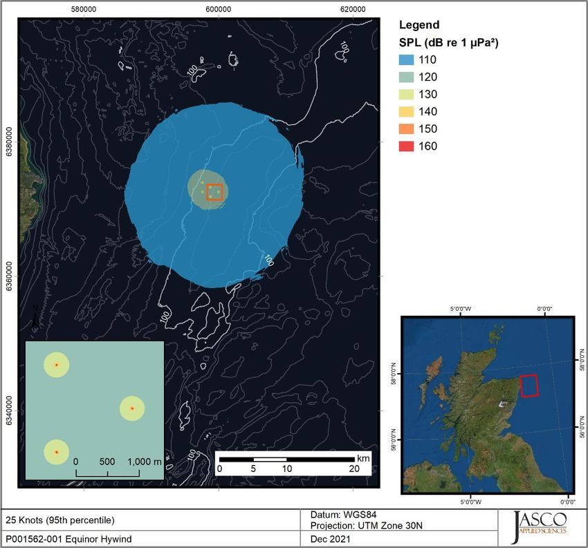
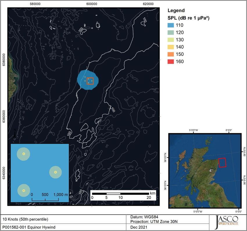
JASCO Applied Sciences Hywind Scotland Floating Offshore Wind Farm

Executive Summary
JASCO Applied Sciences conducted a sound source characterisation study of the Hywind Scotland
floating offshore wind farm, involving in situ acoustic recording over three winter months
(October 2020 to January 2021) at the Hywind site and at a Control site 14 km away. JASCO field
engineers conducted the deployment and retrieval of the recording instrumentation from the Hywind
support vessel, MCS SWATH 1 (out of Peterhead) under the oversight of the Hywind Operations
Room.
The recording instrument at the Hywind site employed a four-hydrophone tetrahedral array to provide
bearing discrimination between sounds from different directions. The location of the recorder was
selected to enable the acoustic isolation of one Hywind structure such that a noise signature from that
unit could be extracted without contamination from the four other floating turbines in the farm. One
further purpose of the directional array was to allow for an analysis of the location of transient noises
from the Hywind mooring system. In a previous study of the Hywind prototype off Norway in 2011,
occasional high amplitude mooring transients were detected but their precise origin was unknown.
The recording program was completed successfully with recovery of a continuously recorded, 24-bit,
acoustic data set (10 Hz to 32 kHz) from each site, a total of approximately 6.6 TB data.
Analysis of the recorded data was conducted to assess the spectral content of the sound signature
from the Hywind structures. Continuous tonal noise, associated with rotating rotor and generator
components below 500 Hz, was clearly evident and showed corelation with wind speed. Temporal
variability in similar frequency tones was suggestive of different concurrent signature for individual
Hywind turbines arriving simultaneously. The other key feature of the overall Hywind noise was the
presence of frequent broadband transient sounds with a median duration of 1.5 s. These transients
were audibly associated with strain and friction in the mooring system and showed a strong positive
corelation in occurrence with wave height. Directional analysis of transient noise from three of the
HYWIDND turbines indicates that the mooring noise is predominantly being generated in mooring
components close to the floating spar and not from components farther down each mooring cable.
A quantitative analysis of the impulsiveness of the soundscape at Hywind was undertaken using an
impulse detector as well as studying the distribution of the per-minute kurtosis. The SEL of each
detected impulse was summed, which showed that the impulsive SEL was generally 6 dB below the
daily total SEL. The mean duration of the impulses was on the order of 1.5 s, longer than the 1.0 s
typically used to identify impulses for the purposes of assessing the effects of sound on hearing. The
soundscape at Hywind had a greater kurtosis than at the Control site; however, the kurtosis was not
high enough to be considered impulsive. Based on these three measures, it is recommended that the
non-impulsive temporary threshold shift (TTS) sound exposure level (SEL) thresholds be applied to
the wind farm sounds.
The total noise levels (tonal and transient) from HS1were extracted and back propagated to derive
decidecade band source levels for a single Hywind Scotland system at five winds speeds between 5
and 25 kn. Unexpectedly, the total noise level from HS1 was higher in 5 kn of wind than at 10 kn of
wind. The resulting median broadband source levels ranged from 162.5 to 167.2 dB re 1 µPa²m² with
the maximum 95th percentile at 25 kn of 172 dB re 1 µPa²m². The HS1 source levels were used to
model a basic noise footprint for the entire five turbine windfarm. The modelling shows that the
distance to the averaged background SPL level (110 dB re1µPa) from the centre of the OWF (i.e.,
where the radiating noise decays to approximately the broadband ambient level) at the quietest state
in 10 kn of wind, was approximately 4 km and in 25 kn of wind it was 13 km. A high-frequency
cetacean (porpoise) would need to remain within 50 m of a turbine for 24 h before there would be a
risk of temporary hearing threshold shift (15 kn wind).

Document 02521 Version 3.0 FINAL 1

JASCO Applied Sciences Hywind Scotland Floating Offshore Wind Farm

1. Introduction
JASCO Applied Sciences (JASCO) was contracted by Equinor Energy AS (Equinor) to undertake a
sound source characterisation (SSC) study for the Hywind floating wind turbine generators (WTG),
located in the North Sea, 25 km to the East of Peterhead, Scotland (Figure 1). Hywind Scotland is the
world’s first operational floating Offshore Wind Farm (OWF) and comprises five WTGs, each mounted
on a spar buoy/pillar that is moored to the seabed by an unballasted catenary system employing three
mooring cables (Figure 2).

Figure 1. Location of the Hywind Scotland offshore floating wind farm.

The diameter of the spar at the water line is approximately 9–10 m, while the diameter of the
submerged section is 14–15 m (Figure 2).
JASCO conducted a similar SSC study for Equinor (Statoil) in 2011 on the Hywind DEMO system off
the coast of Stavanger, Norway. That study identified several tonal elements to the sound signature
and an additional transient ‘snapping/clicking’ noise, potentially associated with the mooring system
(Martin et al. 2011). The principal aim of this 2020 study was to record an operational noise profile for
the larger Hywind Scotland system and back-propagate this data to extract a source spectrum for an
individual Hywind unit. A secondary aim was to determine whether the broadband mooring transients
that were detected from the Hywind DEMO system, were still present.

Document 02521 Version 3.0 FINAL 2

JASCO Applied Sciences Hywind Scotland Floating Offshore Wind Farm

Figure 2. Image of the Hywind floating wind turbine, mooring and power transfer cables.

This SSC study employed two JASCO recording instruments on the seabed for three months over
autumn to winter 2020–2021 to continuously capture noise from the windfarm site and a control site
remote to the wind farm. The recorder located in the wind farm was fitted with a directional array of
four hydrophones to provide acoustic discrimination in bearing and elevation between the
considerable number and spatial distribution of possible noise sources.
The control recorder was retrieved in January 2021 and the Hywind mooring in July 2021. A detailed
analysis of the data was carried out in autumn that year. A bespoke automated code, tailored to the
frequency range and environmental conditions at the wind farm, was developed to process the
directional data because the wide distribution of potential noise sources within the wind farm was
considerable (notably the spread of each mooring system).

Document 02521 Version 3.0 FINAL 3

JASCO Applied Sciences Hywind Scotland Floating Offshore Wind Farm

2. Methods

2.1. Acoustic Data Acquisition
Underwater sound was recorded with two JASCO Autonomous Multichannel Acoustic Recorders
(AMAR) mounted on simple baseplate moorings. A single AMAR G4 with a quad-hydrophone
directional array on a static frame, was deployed within the Hywind site and a second AMAR G3 with a
single omni-directional hydrophone was deployed at a remote location to gather ‘control’ ambient
noise.

2.1.1. Deployment
Both moorings were lowered to the seabed from the Hywind service vessel (MCS SWATH 1), and the
lowering line was disconnected from the mooring’s lifting ring by activation of an acoustic release. The
omni-directional control site recorder did not require any specific orientation, but the Hywind site
recorder, with its four-hydrophone array, did require orientation to enable bearing alignment and
accuracy. The orientation process was applied retrospectively during post-processing of the data by
aligning known positions from the AIS track of the SWATH 1 with the directional vessel noise as well
as corroborating the alignment with the known positions of the Hywind turbines

Figure 3. Baseplate mooring design with the deployment assembly shown.

Document 02521 Version 3.0 FINAL 4

JASCO Applied Sciences Hywind Scotland Floating Offshore Wind Farm

The Control site was selected to be sufficiently distant from the Hywind OWF (~13 km to the
northeast) to exclude significant levels of noise from the turbines and moorings but close enough to
provide representative ambient noise levels for that depth and region of the North Sea. The control
location was also close to the intersection of two seabed pipelines to reduce the risk of trawling loss of
the instrument (Figure 4).

Figure 4. Map showing the Hywind and Control site locations.

The Hywind site recording location was selected specifically to isolate one Hywind turbine east of the
recording instrument such that the array’s directional properties could be used to extract the noise
signature from a single Hywind system without contamination from the other turbines in the farm. The
isolated system selected was HS1 and the mooring was deployed to the west northwest at a 642 m
distance (Figure 5). The exact distance between the AMAR and HS1 did not have to be pre-defined
for back-propagation purposes, as long as it was known. This simplified the deployment process for
the mooring.

Figure 5. AMAR position within the Hywind OWF. Red dashed lines identify the bearing isolation of HS1 and its
mooring system to the East

Document 02521 Version 3.0 FINAL 5

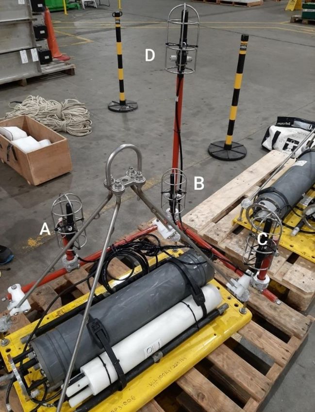
JASCO Applied Sciences Hywind Scotland Floating Offshore Wind Farm

2.1.2. Recording Parameters
Both AMARs were fitted with M36-V35-100 omni-directional hydrophones (with a nominal sensitivity of
−165 dBV with preamp) from GeoSpectrum Technologies Inc. (GTI). Each hydrophone was protected
by a cage covered with a shroud to minimize any flow noise. For the Hywind station, the four
hydrophones were fixed in a tetrahedral arrangement to allow determination of the time of arrivals
from different directions (Figure 6). The relative distance of each hydrophone on the support structure
was calculated and precisely set to support post-processing directional calculations (Table 1).

Table 1. Relative distances of the four hydrophones (as labelled in Figure 6) mounted on the Hywind monitoring
station.

 Hydrophone ID Length (mm)
 A-B 481
 A-D 724
 B-D 595
 B-C 482
 C-A 647
 C-D 717

Figure 6. Photo of the Hywind baseplate before deployment with fitted AMAR G4 (white tube), battery back (grey
tube) and tetrahedral hydrophone array mounted on a static frame (red tubes).

Document 02521 Version 3.0 FINAL 6

JASCO Applied Sciences Hywind Scotland Floating Offshore Wind Farm

The AMARs recorded continuously at a sample rate of 64,000 Hz to return a recorded bandwidth of
10 to 32,000 Hz. The recording channel had 24-bit resolution with a spectral noise floor of 20 dB re
1 µPa2/Hz and a nominal ceiling of 165 dB re 1 µPa. Acoustic data were stored on 512 GB of internal
solid-state flash memory.
Each AMAR was calibrated before deployment and after retrieval with a pistonphone type 42AC
precision sound source (G.R.A.S. Sound & Vibration A/S) (Figure 7). The pistonphone calibrator
produces a constant tone at 250 Hz at a fixed distance from the hydrophone sensor in an airtight
space with known volume. The recorded level of the reference tone on the AMAR yields the system
gain for the AMAR and hydrophone. To determine absolute sound pressure levels, this gain is applied
during data analysis. Typical calibration variance using this method is less than 0.7 dB absolute
pressure.

Figure 7. GRAS 42 AC Pistonphone, sleeve coupler and hydrophone

Data was recorded continuously (i.e., 24 h per day) from 21 Oct 2020 to 24 Jan 2021 at both sites, for
the required monitoring duration of 96 days (Table 2) after which the solid-state memory in each
system was full. The remaining power in the battery pack would have depleted slowly thereafter until
exhausted. The total volume of data collected was approximately 6.6 TB.

Table 2. AMAR deployment and retrieval dates and locations. Retrieval time indicates the time at which the
retrieval procedure was initiated.

 Water
Location Deployment† Retrieval† Latitude Longitude Easting* Northing*
 depth (m)
 21 Oct 2020 15 Jul 2021
 Hywind 57° 29.109’ N 001° 20.571’ E 599348.894 6372604.308 112
 13:44 10.30
 21 Oct 2020 24 Jan 2021
 Control 57° 31.801’ N 001° 07.580’ E 612189.991 6377935.635 95
 11:43 13:05
†
 Time in UTC
* UTM 30N (WGS84)

2.1.3. Retrieval
Retrieval of this mooring design is typically achieved through activation of the separate pop-up
acoustic assembly, connected by ground line to the baseplate. The pop-up float is recovered on board
the vessel and the secondary anchor lifted to access the ground line which, in turn, is used to lift the
baseplate to the surface.
The Control site mooring was retrieved on 24 Jan 2021 (Table 2) by a JASCO field team aboard the
SWATH 1 exactly in line with this procedure. However, during retrieval of the Hywind site mooring on
the same day the ground line became entangled in a hull fitting below the waterline of the SWATH 1
as the baseplate was being winched to the surface and the vessel moved astern from the mooring
position. When the line could not be freed, it had to be cut for vessel safety reasons and the baseplate
mooring fell back to the seabed. The position was recorded at the time. Recovery of the mooring was
finally achieved on 15 Jul 2021 by a Remotely Operated Vehicle (ROV) deployed from the Havila
Venus, on task for Equinor. The mooring had remained upright and inert on the seabed, exactly where
it had fallen from below the SWATH 1. The AMAR was undamaged, and the all the data were
recovered from the on-board memory.

Document 02521 Version 3.0 FINAL 7

JASCO Applied Sciences Hywind Scotland Floating Offshore Wind Farm

2.2. Acoustic Data Analysis
The acoustic data analysis methods for basic metrics are contained in Appendix A. Acoustic
terminology and analysis are in accordance with ISO standard 18405 (ISO 2017).
Bearings and distances between the Hywind recording instrument and each of the turbines were
calculated using mapping software Global Mapper (Table 3) and used as a reference to calculate the
bearing angles of each of the four hydrophones deployed on the tetrahedral structure. Additionally,
the acoustic signature of the SWATH 1 was tracked on the Hywind array immediately after
deployment and correlated with actual bearings derived from positions in the vessel’s GPS track log.
This provided additional directional confirmation of the orientation of the hydrophone array. A
description of the directional analysis is contained in Appendix B.

Table 3. Distances and bearings of each of the Hywind wind turbine generators (WTGs) from the Autonomous
Multichannel Acoustic Recorder (AMAR) deployed within the wind farm.

 Location Distance (m) Bearing ()
 HS-1 605 095
 HS-2 880 318
 HS-3 2242 308
 HS-4 951 1799
 HS-5 1799 269

Impulses were detected in the data to quantify the number of impulses per hour for comparison to the
mean hourly wind speed, as well as to quantify the impulsive daily SEL (with auditory frequency
weighting). The analysis of continuous sounds from the floating turbines indicated that there were two
strong tonal sounds below 100 Hz (see Section 4) whose energy would both affect the impulse
detector’s performance and should not be included with an analysis of impulsive energy. Therefore,
the data were pre-filtered with a high-pass filter before impulse analysis. This finite impulse response
filter was designed using MATLAB’s filter designer application with the Kaiser Window method, a stop
band frequency of 85 Hz, passband frequency of 100 Hz, and stopband attenuation of 80 dB. The
impulse detector is based on a Teager-Kaiser energy detector. The filtered time-series were squared,
summed over a 100 ms window, divided by the number of samples in the window to generate a
100 ms energy time series. The 100 ms time series was divided by its mean value for each 20 s buffer
of data that is passed to the Teager-Kaiser operator (Kaiser 1990, Kandia and Stylianou 2006).
Normalising the 20 s buffer by its mean value allows us to use a fixed threshold that is independent of
the absolute magnitude of the raw time-series data. When the Teager-Kaiser operator exceeded the
detector threshold, set empirically to 15, an impulse was detected. The processing then selected a
2.0 s window from the filtered time series centred on the impulse detection time and computed the
decidecade sound exposure levels for the impulse. The detector was configured with a ‘lock-out’ of
1.0 s after a strike was identified to minimize false alarms on multipath arrivals.

Kurtosis is another approach used in this study to characterize impulsive sounds. Kurtosis ( β) is
defined as the ratio of the fourth moment to the squared second moment of the instantaneous sound
pressure:
 1
 ∑ ( − )4
 = (1)
 2
 1
 [ ∑ ( − )2 ]
where pi is the ith sample of instantaneous sound pressure, p is the arithmetic mean of sound
pressure, and N is the number of data samples in the analysis window that affects resulting value for β.
As suggested in Martin et al. (2020), 1 min analysis window was used for this project. Kurtosis of 3
represents random Gaussian noise, while kurtosis of 40 is used as a threshold for determining if a
soundscape is impulsive for purposes of determining if an impulsive or non-impulsive hearing

Document 02521 Version 3.0 FINAL 8

JASCO Applied Sciences Hywind Scotland Floating Offshore Wind Farm

threshold shift threshold is exceeded (NFMS 2018). Kurtosis for wind driven underwater ambient
noise is also ~3.

Document 02521 Version 3.0 FINAL 9

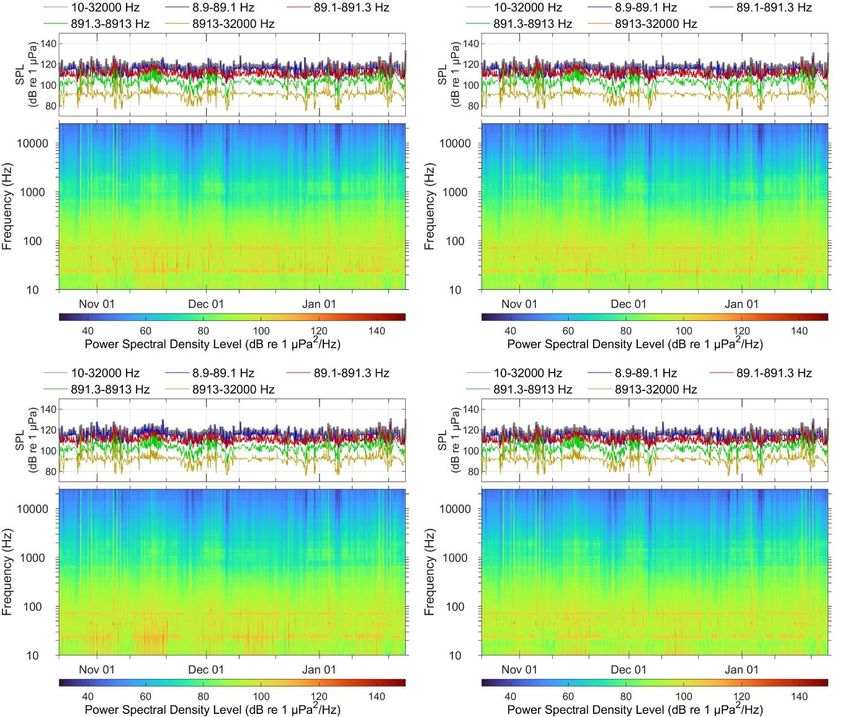
JASCO Applied Sciences Hywind Scotland Floating Offshore Wind Farm

3. Results

3.1. Total Sound Levels
This section presents the total sound levels (non-directional) from each of the sites to verify the quality
of the recordings and as a summary of the received sound levels. We present the results in four ways:
1. Band-level plots: These strip charts show the averaged received sound levels as a function of
 time within a given frequency band. We show the total sound level (10–32000 Hz) and the decade
 bands for 8.9–89.1, 89–891, 891–8913, and 8913–32000 Hz. The 8.9–89.1 Hz band is associated
 with fin, sei, and blue whales, large shipping vessels, seismic surveys, and mooring noise. The 89–
 891 Hz band is generally associated with wind and wave noise, but can also include sounds from
 minke, right, and humpback whales, nearby vessels, and seismic surveys. Sounds above 1000 Hz
 include humpback whales, pilot whale and dolphin whistles, and wind and wave noise.
2. Long-term Spectral Averages (LTSAs): LTSAs use colour to show power spectral density levels
 as a function of time (x-axis) and frequency (y-axis). The LTSAs are excellent summaries of the
 temporal and frequency variability in the data.
3. Distribution of decidecade band SPL: These box-and-whisker plots shows the average and
 extreme sound levels in each decidecade-band. As discussed in Appendix A, decidecade-bands
 are representative of the hearing bands of many mammals. They are often used as the
 bandwidths for expressing the source level of broadband sounds like shipping and seismic
 surveys. The distribution of decidecade noise levels can be used as the noise floor for modelling
 the detection of vessels or marine mammal calls.
4. Power Spectral Densities (PSDs): PSDs show the statistical sound levels in 1 Hz frequency bins.
 These levels can be directly compared to the Wenz curves. We also plot the spectral probability
 density (Merchant et al. 2013) to assess whether the distribution is multi-modal.
Figures for the Hywind site are presented for one of the four hydrophone channels in this section (i.e.,
omni-directional) for ease of comparison with the control site. The data recorded on all four channels
of the Hywind station produced very similar results. Individual results for all channels are presented in
Appendix B.1.
Figure 8 presents band levels and LTSAs for each site. The control site’s LTSA shows lower levels
across the full frequency spectrum and, in particular, below 1kHz. At the Hywind site, sound levels
between 100–120 dB are noticeable throughout the deployment between 8.9–300 Hz.
Transient broadband increases in energy, associated with marine vessels are noticeable at both the
control and the Hywind site. The two obvious horizontal bands (at 25 and 79 Hz) present for almost
the entire deployment at the Hywind site are also noticeable characteristics.

Figure 8. Acoustic summary at the control (left) and Hywind (right, channel 0) monitoring stations.

Document 02521 Version 3.0 FINAL 10

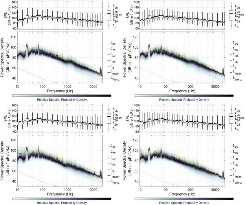
JASCO Applied Sciences Hywind Scotland Floating Offshore Wind Farm

The most obvious differentiating feature of the PSD and decidecade-band analysis (Figure 9) are the
two large peaks at 25 and 75 Hz seen at the Hywind site but mostly absent at the Control site. Median
PSD levels in these two bands were 10–20 dB higher than at the adjacent frequencies, indicating a
very significant increase in sound pressure levels. These noises are therefore important contributors
and features of the soundscape, and they are most likely related to Hywind turbine and electricity
transmission system noise (Figure 10) in combination with the relatively regular mooring noise. A
small peak at 25 Hz is visible in the PSD of the control site, which may indicate a degree of residual
audibility of this component of the Hywind noise at that distance.
At the Hywind site, several additional peaks can be seen between 100–400 Hz. These are believed to
be associated with regular but transient sounds described as ‘creaks’, ‘snaps’ and ‘rattles’ thought to
be associated with components of the Hywind mooring system. The occurrence of these generally
broadband transients is irregular, and their duration also shows some variability with typical durations
between 0.2 and 1.0 s.
Several distinct peaks are noticeable at both sites between 20–32 kHz. These sounds were manually
investigated by generating spectrograms for selected recordings and were confirmed as matching the
frequency peaks seen in the PSD, as shown in Appendix B.1. Given both the high-frequency, regular
transmission characteristics and equal presence at both sites, in addition to evidence of concurrent
vessel noise, it is thought that they are unrelated specifically to Hywind operational noise and are most
likely to be some form of vessel mounted echo sounder or similar transmitting device.
Generally, the shape of the PSD percentiles was similar at both stations, except for those identified
peaks, and below 20 Hz where the control site has a wider statistical spread of levels, visible in the
spectral probability density shading. This is most likely due to the proximity of passing vessels that
would navigate around the Hywind site but were able to transit directly over the control site recorder.

Figure 9. (Bottom) Power spectral density levels and (top) decidecade-octave-band sound pressure level (SPL)
(left) at the control (left) and Hywind (right) monitoring stations. Values for each percentile appear in Tables F-1
and F-2.

Document 02521 Version 3.0 FINAL 11

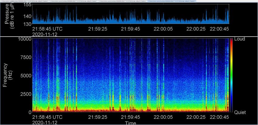
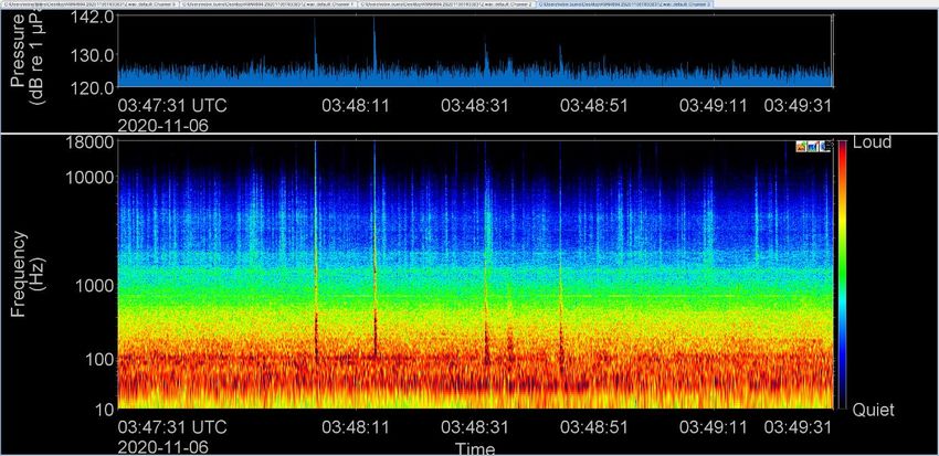
JASCO Applied Sciences Hywind Scotland Floating Offshore Wind Farm

Figure 10. Amplitude (top) and spectrogram (bottom) of a 30 s section of a recording from the Hywind site from
7 Dec 2020 showing the dominant 25 and 75 Hz tones. A fainter harmonic is also visible between these two
primary frequencies.

3.2. Comparison with Environmental Conditions
Sound levels in representative decidecade bands (Ddec) from the Control and Hywind stations were
compared to NORA10 (operated by the Norwegian Meteorological Institute) environmental conditions
at the P2 location (Figure 12), including wind speed, wind direction, and significant wave height (Hs) to
assess for compliance with averaged ocean conditions. From the environmental parameters, the wind
speed and wave height have a strong positive correlation, which reflect natural conditions of wind
generated waves. For the Control site, the strongest positive relationships are at the highest two
decidecade bands, when compared to either the wind speed or wave height. These correspond with
the frequencies impacted by sea state, as per the Wenz curves (Figure 13). There is also a moderate
positive correlation with the lowest frequency band, which is within the range impacted by surface
waves. At the Hywind station, there are strong-moderate positive correlations with all frequency
bands. The most substantial changes are the increase in correlation between wind speed and the
lowest two decidecade bands. These increases are attributed to the finding that turbine and mooring
noise increases with wind speed. There are slight decreases at Hywind in correlation strength of either
wind speed or wave height at the highest two decidecade bands compared to the Control, for which a
possible explanation could be a difference in sea state at the two stations, but the difference is small
and there is unlikely to be a significant increase in sea state at the control site, despite the slightly
longer fetch for the prevailing wind to the control site.
The correlograms below present a corelation analysis for each of the environmental factors and noise
bands shown. The variable names on the diagonal become the vertical and horizontal axis labels for
each grid panel. The scatter plots in the upper right compare each variable. The circles in the bottom
left show the strength of the correlation of variable pairs simultaneously by amount of circle filled
(clockwise from top if positive, anti-clockwise if negative), and darkness of colour (pale-to-dark
blue/red). Blue indicates a positive correlation, and red a negative. For example, wind speed and wave
height have a strong positive correlation represented by the dark blue colour and ~80% fill. The darker
the blue colour, the greater the positive correlation, based on an automated colour scale set by the
range of data. Wind direction and the 80 Hz decidecade have a weakly negative correlation
exemplified by the small fraction of pale red fill.

Document 02521 Version 3.0 FINAL 12

JASCO Applied Sciences Hywind Scotland Floating Offshore Wind Farm

Figure 11. Correlograms comparing decidecade sound levels with environmental parameters for the Control site.

Document 02521 Version 3.0 FINAL 13

JASCO Applied Sciences Hywind Scotland Floating Offshore Wind Farm

Figure 12. Correlograms comparing decidecade sound levels with environmental parameters for the Hywind
stations.

Document 02521 Version 3.0 FINAL 14

JASCO Applied Sciences Hywind Scotland Floating Offshore Wind Farm

Figure 13. Wenz curves describing pressure spectral density levels of marine ambient sound from weather, wind,
geologic activity, and commercial shipping. Thick lines indicate limits of prevailing noise. Figure reproduced from
National Research Council (2003) and Wenz (1962).

Document 02521 Version 3.0 FINAL 15

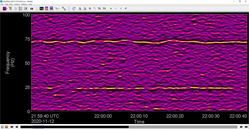
JASCO Applied Sciences Hywind Scotland Floating Offshore Wind Farm

3.3. Acoustic Analysis of Recorded Noise
Acoustic analysis of the recorded data was carried out using a combination of auto-processed event
detection, manual spectral analysis of events, and Passive Aural Listening. Operational logs for the
Hywind turbines were received towards the end of this analysis work, which provided some context
regarding operating modes for the turbines.
Three separate categories of noise were determined from the analysis—firstly mechanical and
electrical noise from the turbines, secondly ‘mooring’ noise and thirdly, noise which could not be
definitively attributed to either category. More detailed directional analysis was conducted following
directional processing of the four array channels, and this is presented separately in Section 3.4.

3.3.1. Turbine Related Noise – Spectral Content
The dominant operational noise from the Hywind turbine system appears to be distinct tonal sounds
(i.e., relatively narrowband, continuous sounds typically associated with running machinery). Two
dominant tones were evident below 100 Hz, and a further set of tones was evident between
approximately 350 and 460 Hz. These tones were moderately stable in frequency, but, at times,
displayed significant instability that is likely to reflect the variability in the RPM of the rotating turbine
as the wind speed fluctuates.
The Hywind generator is understood to be directly linked (i.e., not geared) to the rotating hub of the
turbine blades and that operational rotation speeds are typically in the region of 10 to 15 RPM.
Interestingly, no corresponding fundamental tonal or harmonically related tones, at the converted
cycles per second frequency, is visible in the data, and it remains unclear exactly which rotating
component of the generator, or other system component, is creating this noise. Unsurprisingly, there
was no evidence of any relatable gearing tones in the recordings.
Figure 14 shows two pairs of the dominant lower-frequency tones (below 100 Hz) indicating that there
are at least two audible Hywind turbines at this time, although there is a potentially third but
considerably weaker tone visible at one or two very short time periods. The analysis comb (at set of
harmonically related lines, in this case separate by 23.84 Hz) is suggestive of a harmonic relationship
between the ~24 and ~74 Hz primary tones (as well as a weaker tone close to 50 Hz), but the
symmetry in oscillation is poor and the significant difference in intensity between what would be the
second harmonic (close to 50 Hz) and the third harmonic (close to 74 Hz) is so significant that this
serves to undermine the harmonic association theory, and it is concluded that these two dominant
tones have separate but closely related origins.
Weaker secondary tonals are evident in Figure 14 between 30 and 50 Hz, and these are explored
further below. Precise correlation of specific tonal features with a specific turbine operational mode
was complicated by the presence of five turbines in the wind farm and the potential for several modes
to be in operation at any one time. Additionally, occasional low-frequency tones from passing vessels
were also routinely seen and had to be identified and excluded. Analysis below was conducted as far
as possible when all five turbines were operating in the same mode.
Directional frequency analysis from the array data indicates that there is often quite a difference
between the acoustic signature for each Hywind system, despite functioning in close proximity to each
other. Significantly, different rotation rates are seen in the analysis that may be due to either small-
scale variability in the wind pressure field, different loading on each generator or different blade pitch
settings (if indeed the blades are controlled), or a combination of these and other factors. Therefore,
no single Hywind noise signature would be representative of all turbines at any one time, and an
overall aggregate noise assessment is necessary to determine the total radiated noise field for the
whole site. This is the approach taken in Section 4 to determine source levels.

Document 02521 Version 3.0 FINAL 16

JASCO Applied Sciences Hywind Scotland Floating Offshore Wind Farm

Figure 14. Primary tonal noise features below 100 Hz of the Hywind site showing overlap of the 25 and 74 Hz
sources from at least two (possibly three) different Hywind turbines.

Figure 15 shows a narrowband analysis over a 2.8 s window of the low-frequency tone at ~74 Hz. The
marked intensity of these tones against the background highlights their dominance in the overall
soundscape.

Figure 15. Narrowband analysis of the meandering tone at ~71 Hz.

Farther up in the acoustic spectrum, between ~350 Hz and 460 Hz, are several additional pronounced
tonal sounds that are also evident in the long-term PSD values for the Hywind site (Figure 9). These
tones are clearly visible in Figure 16 along with the primary tones below 100 Hz but showing little
direct association with them. There is a temporal oscillation in intensity that is not mirrored with the
lower frequency tones and no direct harmonic association again suggesting a different but still related
origin. It is unknown if there is additional machinery on the Hywind structure, such as a bilge pump or

Document 02521 Version 3.0 FINAL 17

JASCO Applied Sciences Hywind Scotland Floating Offshore Wind Farm

any other rotational machinery but given that there is no gearing in the turbine drive train, it is thought
that these higher frequency tones are either related to another mechanical system in the Hywind
structure or peripherally related elements of the generator. A fuller understanding of the rotation
speed of all the components within the turbine may allow for a closer understanding of the precise
source of each noise.

Figure 16. Additional higher frequency tones displaying a regular oscillation in intensity over a 1 min period.

Weaker, but still relatively persistent, tones within the noise field have also been identified but appear
to be unrelated directly to the primary rotational tones that dominate the signature and are not always
visible even when the sets of primary dominant tones are. These additional elements are possibly
associated with the power generation mode, as they are not continuously present but do display a
degree of intensity correlation with wind speed (Figure 17). They have no obvious harmonic
relationship with the rotational primary tones and could be more related to electrical transformer or
other power handling equipment. This additional noise is sufficiently loud in the measured band levels
at different wind speeds to be a significant contributor to the overall radiated noise field and features
again in the source level derivation work in Section 4.

Document 02521 Version 3.0 FINAL 18

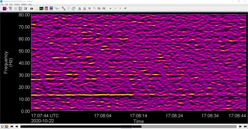
JASCO Applied Sciences Hywind Scotland Floating Offshore Wind Farm

Figure 17. Additional tonal content evident during power generation mode. Centroid frequency 13.46 Hz.
Emissions are strong with harmonic structure

A longer time series over 20 minutes (Figure 18) in power generation mode, shows the relative
stability of the dominant tonal noise and also highlights what is likely to be a small degree of variability
in frequency between two different turbines in the higher frequency tones (~380–460 Hz). At this
relatively low wind speed, evidence of the weaker power generation tones, seen mostly below 100 Hz,
is somewhat masked due to significant shading from the very strong ~24 and ~75 Hz primary tones.
As wind speed increases, these secondary, low-frequency tones start to become more apparent.

Figure 18. A 20 min time series in power generation mode showing the dominant tonal noise elements of the
overall wind farm signature.

Document 02521 Version 3.0 FINAL 19

JASCO Applied Sciences Hywind Scotland Floating Offshore Wind Farm

3.3.2. Mooring System Noise
One of the aims of the project was to understand whether the ‘snapping’ transients, believed to be
caused by the prototype mooring system, were still present. Analysis of the acoustic data revealed a
significant amount of mooring noise, but there was very little evidence of the intense, very sharp,
impulsive ‘snap’ sound that was previously detected.
However, there was considerably more mooring-related noise than had been found in the Hywind
Demo recordings, notwithstanding the fact that there are five Hywind systems at the site rather than
just one. The new mooring transients are typically broadband, repetitive, and considerably less
impulsive and fall into three distinct types, described from aural analysis as ‘creaks’, ‘bangs’, and
‘rattles’. Figure 19 shows an example of four ‘bang’ transients of varying duration from 0.3 to 1.0 s.
There is a sense from audio analysis of tension release in many of these noises, supported by the
rapid onset and significant intensity of the sound seen in the spectrograms. Figure 20 shows an
example of a ‘creak’ transient.
Further detailed directional analysis was conducted on the transient noises resulting in
characterisation and assignment of specific noise types to individual Hywind systems within the wind
farm. The directional noise analysis provides an additional insight into the nature and source of
mooring noise and is presented in Section 3.4. An analysis of the impulsiveness of the sounds is
presented in Section 3.7.

Figure 19. Amplitude (top) and spectrogram (bottom) of a 30 s section of a recording from the Hywind site from
7 Dec 2020 showing four impulsive mooring transients.

Document 02521 Version 3.0 FINAL 20