Global human-made mass exceeds all living biomass - MIT
←
→
Page content transcription
If your browser does not render page correctly, please read the page content below
Article

Global human-made mass exceeds all living
biomass

https://doi.org/10.1038/s41586-020-3010-5                     Emily Elhacham1, Liad Ben-Uri1, Jonathan Grozovski1, Yinon M. Bar-On1 & Ron Milo1 ✉

Received: 1 November 2019

Accepted: 9 October 2020                                      Humanity has become a dominant force in shaping the face of Earth1–9. An emerging
Published online: 9 December 2020                             question is how the overall material output of human activities compares to the
                                                              overall natural biomass. Here we quantify the human-made mass, referred to as
    Check for updates
                                                              ‘anthropogenic mass’, and compare it to the overall living biomass on Earth, which
                                                              currently equals approximately 1.1 teratonnes10,11. We find that Earth is exactly at the
                                                              crossover point; in the year 2020 (± 6), the anthropogenic mass, which has recently
                                                              doubled roughly every 20 years, will surpass all global living biomass. On average,
                                                              for each person on the globe, anthropogenic mass equal to more than his or her
                                                              bodyweight is produced every week. This quantification of the human enterprise
                                                              gives a mass-based quantitative and symbolic characterization of the human-induced
                                                              epoch of the Anthropocene.

The face of Earth in the twenty-first century is affected in an unprec-                       input and output material flows. A recent study used and expanded the
edented manner by the activities of humanity and the production                               framework to quantify global values for the human-made mass flows
and accumulation of human-made objects. Given the limitations of                              and standing stocks21,22 (objects that have been built by humans and
human cognition in the face of the immensity of the globe and the                             are still in use: buildings, roads, machines and so on).
seeming infinity of the natural world, it is desirable to provide a rigor-                        These advances in the global quantification of both living biomass
ous and objective measure of the overall balance between the living                           and human-made mass provide an opportunity to conduct an inte-
and human-made. However, in spite of pioneering efforts1–8, we lack a                         grated comparison of the two, which is the primary focus of this paper.
holistic picture that quantifies and compares the composition of the                          Comparing biomass with human-made mass necessitates bringing
world in terms of both biological and human-made mass.                                        together objects with different attributes, going beyond comparing
   A case in point is our planet’s biomass. While the mass of humans is                       apples and oranges to compare apples and mobile phones. However,
only about 0.01% of global biomass, our civilization had already had                          we find that because living biomass surrounds and supports humanity,
a substantial and diverse impact on it by 3,000 years ago9. Since the                         it is a natural logical reference point to give a quantitative perspective
first agricultural revolution, humanity has roughly halved the mass                           on the mass that humanity has produced. By contrasting human-made
of plants, from approximately two teratonnes (Tt, units of 1012 tonne;                        mass and biomass over time, we present an additional dimension to the
where estimates are on a dry-mass basis) down to the current value10 of                       ongoing assessment of the evolving human dominance on Earth and
approximately 1 Tt. While modern agriculture utilizes an increasing land                      provide a visual and symbolic characterization of the Anthropocene.
area for growing crops, the total mass of domesticated crops (about                               We estimate the global biomass and human-made mass from 1900
0.01 Tt)11 is vastly outweighed by the loss of plant mass resulting from                      in units of teratonnes (which equal 1018 grams) of dry weight (that
deforestation, forest management and other land-use changes10. These                          is, excluding water). Biomass represents the overall global mass of
trends in global biomass have affected the carbon cycle and human                             all living taxa11. Anthropogenic mass is defined as the mass embed-
health12,13. Additional human actions, including livestock husbandry,                         ded in inanimate solid objects made by humans (that have not been
hunting and overfishing, have also strongly affected the masses of                            demolished or taken out of service, which we define as ‘anthropogenic
various other taxa11,14,15. A recent survey of Earth’s remaining living                       mass waste’). The mass of humans themselves (and their livestock)
biomass11 has found that, on a mass basis, plants constitute the vast                         is naturally accounted for as part of the global biomass. In any case
majority (about 90%)16, followed by bacteria, fungi, archaea, protists,                       their mass contribution is negligible. Figure 1 shows changes in bio-
and animals.                                                                                  mass and anthropogenic mass over the studied period. It is clear that
   Beyond biomass, as the global effect of humanity accelerates, it is                        the two exhibit markedly different temporal dynamics. Over the past
becoming ever more imperative to quantitatively assess and monitor                            100 years, anthropogenic mass has increased rapidly—doubling in
the material flows of our socioeconomic system, also known as the                             a Moore-law-like fashion approximately every 20 years—in contrast
socioeconomic metabolism17,18. This quantification is at the heart of                         to total biomass, which has not changed as markedly (affected by a
the economy-wide material flow analysis framework, under the field of                         complex interplay of deforestation, afforestation and the rising CO2
industrial ecology, which is based on mass balance accounting19,20. This                      fertilization effect, among other things). The accumulation of anthro-
extensively developed framework enables researchers to investigate                            pogenic mass has now reached 30 Gt per year, based on the average for
the material basis of society, on local and global scales. It includes the                    the past 5 years. This corresponds to each person on the globe produc-
mass and composition of socioeconomic material stocks as well as                              ing more than his or her body weight in anthropogenic mass every

Department of Plant and Environmental Sciences, Weizmann Institute of Science, Rehovot, Israel. ✉e-mail: ron.milo@weizmann.ac.il
1

442 | Nature | Vol 588 | 17 December 2020
1.6
                                                                                                               3
                  1.4

                  1.2                                             Biomass            2020 ± 6
                                                                                                                      Biomass (wet)                                       2037 ± 10
Dry weight (Tt)

                  1.0
                                                                                                                                                                        2031 ± 9
                                                                                                               2
                  0.8

                                                                                                 Weight (Tt)
                  0.6      Other (for example, plastic)
                           Metals
                                                              Anthropogenic                                           Biomass (dry)                                 2020 ± 6
                  0.4      Asphalt
                                                                  mass
                           Bricks
                                                                                                               1                                             2013 ± 5
                  0.2      Aggregates (for example, gravel)
                           Concrete
                   0                                                                                                  Anthropogenic mass waste
                    1900     1920          1940           1960       1980     2000        2020
                                                                                                                      Anthropogenic mass
                                                           Year
                                                                                                               0
Fig. 1 | Biomass and anthropogenic mass estimates since the beginning of                                       1900   1920     1940     1960          1980   2000        2020
the twentieth century on a dry-mass basis. The green line shows the total
                                                                                                                                               Year
weight of the biomass (dashed green lines, ±1 s.d.). Anthropogenic mass weight
is plotted as an area chart, where the heights of the coloured areas represent                   Fig. 2 | Biomass (dry and wet), anthropogenic mass and anthropogenic
the mass of the corresponding category accumulated until that year. The                          mass waste estimates since the beginning of the twentieth century. Green
anthropogenic mass presented here is grouped into six major categories. The                      lines show the total weight of biomass (± 1 s.d.). Anthropogenic mass weight is
year 2020 ± 6 marks the time at which biomass is exceeded by anthropogenic                       plotted as an area chart. The wet-weight estimate is based on the results
mass. Anthropogenic mass data since 1900 were obtained from ref. 22, at a                        presented in Fig. 1 and the respective water content of major components
single-year resolution. The current biomass value is based on ref. 11, which for                 (see Methods). The year 2013 ± 5 marks the time at which the dry biomass is
plants relies on the estimate of ref. 10, which updates earlier, mostly higher                   exceeded by the anthropogenic mass, including waste. The years 2037 ± 10 and
estimates. The uncertainty of the year of intersection was derived using a                       2031 ± 9 mark the times at which the wet biomass is exceeded by the
Monte Carlo simulation, with 10,000 repeats (see Methods). Data were                             anthropogenic mass and the total produced anthropogenic mass, respectively.
extrapolated for the years 2015–2025 (lighter area; see Methods). For a detailed                 The uncertainties of the years of intersection were derived using a Monte Carlo
view of the stock accumulation for the ‘metals’ and ‘other’ groups, see                          simulation, with 10,000 repeats (see Methods). Weights are extrapolated for
Extended Data Figs. 4, 5.                                                                        the years 2015–2037 (lighter area; see Methods).

week. As a result, the gap between anthropogenic mass and overall                                of produced plastic is greater than the overall mass of all terrestrial and
biomass has quickly shrunk. We find that the two curves intersect in                             marine animals combined.
the year 2020 ± 6 years (1 s.d.), at which point anthropogenic mass will
surpass biomass.
   The anthropogenic mass is divided into sub-groups, which constitute                           Discussion
human-made objects22 (Extended Data Table 1): concrete, aggregates,                              At the beginning of the twentieth century, anthropogenic mass was
bricks, asphalt, metals and ‘other’ components (wood used for paper                              equal to only 3% of global biomass, with a massive difference of about 1.1
and industry, glass and plastic). As shown in Fig. 1, the anthropogenic                          Tt on a dry-weight basis. About 120 years later, in 2020, anthropogenic
mass is dominated by concrete and aggregates (such as gravel). The                               mass is exceeding overall biomass in the world. As shown above, the
crossover year has an uncertainty that arises from an uncertainty                                exact timing of the point at which anthropogenic mass surpasses living
of ±16% for overall biomass and ±6% for anthropogenic mass, with all                             biomass is sensitive to the definitions of biomass and anthropogenic
uncertainties reported as ±1 s.d. The analysis shown in Fig. 1 presents                          mass; for example, whether they are defined on a wet- or dry-mass
biomass on a dry-weight basis. To provide a complementary point                                  basis. However, we find that under a range of definitions, the point of
of view, Fig. 2 shows biomass on a wet-mass basis and compares it to                             transition is in either the past decade or the next two (Supplementary
anthropogenic mass and accumulated anthropogenic mass waste.                                     Information section 1, Extended Data Fig. 1).
Anthropogenic mass waste is anthropogenic mass that has been demol-                                 The analysis of the changes in anthropogenic mass composition
ished or taken out of service (time-integrated cumulative solid waste                            across the studied period highlights specific trends (Extended Data
flow, subsequently referred to as simply ‘waste’. This does not include                          Fig. 2). For example, the gradual shift from construction dominated
unused mass excavated through mining, landscape modification and so                              by bricks to concrete, which tilted in favour of concrete in the
on). When we include the waste component, dry biomass is surpassed                               mid-1950s, is clear, as is the emergence of asphalt as a major road
at 2013 (± 5 years). On a wet-weight basis, the current biomass stands at                        pavement material from the 1960s. Analysis of the rate of accumula-
approximately 2.2 Tt and is expected to be exceeded by anthropogenic                             tion of anthropogenic mass further provides a material-based view
mass by the 2030s, with (2031 ± 9 years) or without (2037 ± 10 years) the                        of humanity’s path since the beginning of the twentieth century, as
inclusion of waste. A sensitivity analysis of the effect of the anthropo-                        shown in Extended Data Fig. 3. Shifts in total anthropogenic mass are
genic mass definition on the intersection year is presented in Extended                          tied to global events, such as world wars and major economic crises.
Data Fig. 1 and detailed in Supplementary Information section 1.                                 Most notably, continuous increases in anthropogenic mass, peaking
   Figure 3 shows some key relations between major human-made and                                at over 5% per year, mark the period immediately following World
biological entities. The two dominant mass categories in our analysis                            War II. This period, frequently termed the ‘Great Acceleration’, is
are buildings and infrastructure (composed of concrete, aggregates,                              characterized by enhanced consumption and urban development23.
bricks and asphalt) and trees and shrubs (the majority of plant mass                             If current trends continue, anthropogenic mass, including waste,
and, therefore, of the overall biomass). We find that the former has                             is expected to exceed 3 Tt by 2040—almost triple the dry biomass
recently outweighed the latter. Similarly, we show that the global mass                          on Earth.

                                                                                                                                 Nature | Vol 588 | 17 December 2020 | 443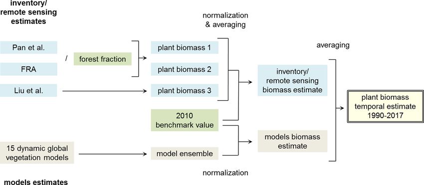
Article
                                                                                       acknowledgements, peer review information; details of author con-
                                                                                       tributions and competing interests; and statements of data and code
                                                                                       availability are available at https://doi.org/10.1038/s41586-020-3010-5.
                Animals                    Plastic
                4 Gt                       8 Gt                                        1.    Ramankutty, N. & Foley, J. A. Estimating historical changes in global land cover: croplands
                                                                                             from 1700 to 1992. Glob. Biogeochem. Cycles 13, 997–1027 (1999).
                                                                                       2.    Krausmann, F. et al. Growth in global materials use, GDP and population during the 20th
                                                                                             century. Ecol. Econ. 68, 2696–2705 (2009).
                                                                                       3.    Matthews, E. The Weight of Nations: Material Outflows from Industrial Economies (World
                                                                                             Resources Inst., 2000).
                                                                                       4.    Smil, V. Harvesting the Biosphere: What We Have Taken from Nature (MIT Press, 2013).
                                                                                       5.    Smil, V. Making the Modern World: Materials and Dematerialization (John Wiley & Sons,
                                                                                             2013).
                                                                                       6.    Haff, P. K. Technology as a geological phenomenon: implications for human well-being.
             Living biomass                     Human-made mass                              Geol. Soc. Lond. Spec. Publ. 395, 301–309 (2014).
                                                                                       7.    Zalasiewicz, J. et al. Scale and diversity of the physical technosphere: a geological
                                                                                             perspective. Anthropocene Rev. 4, 9–22 (2017).
                                                                                       8.    Zalasiewicz, J., Waters, C. N., Williams, M. & Summerhayes, C. The Anthropocene as a
                                                                                             Geological Time Unit: A Guide to the Scientific Evidence and Current Debate (Cambridge
                                                                                             Univ. Press, 2018).
             Trees and                     Buildings and                               9.    Stephens, L. et al. Archaeological assessment reveals Earth’s early transformation
             shrubs                        infrastructure                                    through land use. Science 365, 897–902 (2019).
             900 Gt                        1,100 Gt                                    10.   Erb, K.-H. et al. Unexpectedly large impact of forest management and grazing on global
                                                                                             vegetation biomass. Nature 553, 73–76 (2018).
                                                                                       11.   Bar-On, Y. M., Phillips, R. & Milo, R. The biomass distribution on Earth. Proc. Natl Acad. Sci.
                                                                                             USA 115, 6506–6511 (2018).
                                                                                       12.   Pan, Y. et al. A large and persistent carbon sink in the world’s forests. Science 333,
                                                                                             988–993 (2011).
                                                                                       13.   Reddington, C. L. et al. Air quality and human health improvements from reductions in
                                                                                             deforestation-related fire in Brazil. Nat. Geosci. 8, 768–771 (2015).
                                                                                       14.   Ceballos, G. & Ehrlich, P. R. Mammal population losses and the extinction crisis. Science
                                                                                             296, 904–907 (2002).
                                                                                       15.   WWF. Living Planet Report–2018: Aiming Higher (WWF, 2018).
                                                                                       16.   Bar-On, Y. M. & Milo, R. Towards a quantitative view of the global ubiquity of biofilms. Nat.
                                                                                             Rev. Microbiol. 17, 199–200 (2019).
                                                                                       17.   Pauliuk, S. & Hertwich, E. G. Socioeconomic metabolism as paradigm for studying the
                                                                                             biophysical basis of human societies. Ecol. Econ. 119, 83–93 (2015).
Fig. 3 | Contrasting key components of global biomass and anthropogenic
                                                                                       18.   Haberl, H. et al. Contributions of sociometabolic research to sustainability science. Nat.
mass in the year 2020 (dry-weight basis). The ratio between the circle areas                 Sustainability 2, 173–184 (2019).
within each pair represents the corresponding mass ratio of the two illustrated        19.   Fischer-Kowalski, M. et al. Methodology and indicators of economy-wide material flow
masses. For visual clarity, the two pairs use different scales. The plastic estimate         accounting. J. Ind. Ecol. 15, 855–876 (2011).
                                                                                       20.   Krausmann, F., Schandl, H., Eisenmenger, N., Giljum, S. & Jackson, T. Material flow
includes plastic currently in use and plastic waste, taking into account recycling.
                                                                                             accounting: measuring global material use for sustainable development. Annu. Rev.
Infrastructure includes the mass of constructed elements, such as roads.                     Environ. Resour. 42, 647–675 (2017).
                                                                                       21.   Krausmann, F. et al. Global socioeconomic material stocks rise 23-fold over the 20th
                                                                                             century and require half of annual resource use. Proc. Natl Acad. Sci. USA 114, 1880–1885
                                                                                             (2017).
   Previous efforts, such as quantifying the human appropriation of net                22.   Krausmann, F., Lauk, C., Haas, W. & Wiedenhofer, D. From resource extraction to outflows
primary production24–26, have focused on the allocation of the biosphere                     of wastes and emissions: the socioeconomic metabolism of the global economy,
productivity flow for human usage. The anthropogenic mass, the accu-                         1900–2015. Glob. Environ. Change 52, 131–140 (2018).
                                                                                       23.   Steffen, W., Broadgate, W., Deutsch, L., Gaffney, O. & Ludwig, C. The trajectory of the
mulation of which is documented in this study, does not arise out of the                     Anthropocene: the great acceleration. Anthropocene Rev. 2, 81–98 (2015).
biomass stock but from the transformation of the orders-of-magnitude                   24.   Vitousek, P. M., Ehrlich, P. R., Ehrlich, A. H. & Matson, P. A. Human appropriation of the
higher stock of mostly rocks and minerals. In doing so, humanity is                          products of photosynthesis. Bioscience 36, 368–373 (1986).
                                                                                       25.   Haberl, H. et al. Quantifying and mapping the human appropriation of net primary
converting near-surface geological deposits into a socially useful form,                     production in Earth’s terrestrial ecosystems. Proc. Natl Acad. Sci. USA 104, 12942–12947
with wide implications for natural habitats, biodiversity, and various                       (2007).
climatic and biogeochemical cycles.                                                    26.   Haberl, H., Erb, K.-H. & Krausmann, F. Human appropriation of net primary production:
                                                                                             patterns, trends, and planetary boundaries. Annu. Rev. Environ. Resour. 39, 363–391
   This study joins recent efforts to quantify and evaluate the scale                        (2014).
and impact of human activities on our planet9,23,27,28. The impacts of                 27.   Vitousek, P. M. Human domination of Earth’s ecosystems. Science 277, 494–499 (1997).
these activities have been so abrupt and considerable that it has been                 28.   Dirzo, R. et al. Defaunation in the Anthropocene. Science 345, 401–406 (2014).
                                                                                       29.   Crutzen, P. J. in Earth System Science in the Anthropocene (eds. Ehlers, E. & Kraft, T.) 13–18
proposed that the current geological epoch be renamed the Anthro-                            (Springer, 2006).
pocene29–32. Our study rigorously and quantitatively substantiates this                30.   Steffen, W., Crutzen, J. & McNeill, J. R. The Anthropocene: are humans now overwhelming
                                                                                             the great forces of Nature? Ambio 36, 614–621 (2007).
proposal. In parallel, it adds another dimension to this discussion—a
                                                                                       31.   Lewis, S. L. & Maslin, M. A. Defining the Anthropocene. Nature 519, 171–180 (2015).
symbolic quantitative demarcation of the transition to our epoch.                      32.   Waters, C. N. et al. The Anthropocene is functionally and stratigraphically distinct from
                                                                                             the Holocene. Science 351, aad2622 (2016).

Online content                                                                         Publisher’s note Springer Nature remains neutral with regard to jurisdictional claims in
                                                                                       published maps and institutional affiliations.
Any methods, additional references, Nature Research reporting sum-
maries, source data, extended data, supplementary information,                         © The Author(s), under exclusive licence to Springer Nature Limited 2020

444 | Nature | Vol 588 | 17 December 2020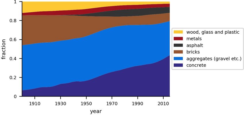
Methods
                                                                                 Biomass change over the years 1900–2017
Anthropogenic mass definition                                                    There have been various previous efforts to quantify global biomass
Our definition of human-made mass, termed here anthropogenic                     using different methodologies, including inventory assessments12,36,
mass, is the mass embedded in inanimate solid objects made by                    remote sensing37 and modelling38,39. In our estimate, we sought to
humans (that have not yet been demolished or taken out of service).              synthesize estimates generated by these different approaches. We
It originates from material flows from the natural environment to the            first estimated plant biomass, which represents about 90% of global
socioeconomic system, accumulated into stocks of artefacts, also                 biomass11. Note that soil carbon is not living biomass and thus is not
known as manufactured capital22. The anthropogenic mass is the                   included in this study.
visible inanimate component of what has been termed the physical
technosphere6,7. As biological components of the physical techno-                Plant biomass estimate for the years 1990–2017. Our plant biomass
sphere, including croplands (for example, rice and hay fields, which             value for 2010, about 0.45 Tt carbon, is based on ref. 11, which relies on
produce flows to the socioeconomic system33) and livestock (part of              the estimate by ref. 10, which consists of the mean of seven maps of
the socioeconomic system), are living natural biological entities, we            global plant biomass that are based on inventories or remote sensing.
classified them under biomass, even though they serve human pur-                 The estimate of about 0.45 Tt carbon, which updates previous, mostly
poses. Conversely, industrial wood, used in construction, was classified         higher, estimates, has been substantiated as the current gold standard
under anthropogenic mass, because it is embedded in human-made                   in ref. 10, which extensively surveyed and integrated different estimates
artefacts. A similar approach for accounting human-made mass is pre-             and approaches.
sented in chapter 1 of ref. 5. A sensitivity analysis of the anthropogenic          To estimate the total plant biomass between 1990 and 2017, we relied
mass definition and its effect on the year of intersection is included           on two approaches. The first approach is based on three main data
in Supplementary Information section 1 and Extended Data Fig. 1, as              sources, using inventory measurements12,36,40 or remote sensing37. The
well as at https://anthropomass.org/analysis/.                                   second is an ensemble of 15 dynamic global vegetation models. To
   The anthropogenic mass was divided into six sub-groups: concrete,             generate our best estimate for total plant biomass, we first calculated a
aggregates, bricks, asphalt, metals and an additional group of other             best estimate for each approach by taking the average of all the sources
components consisting of wood, glass and plastic. The aggregates                 within the same approach and then taking the average of the best esti-
group includes the gravel and sand that serve as bedding for roads               mates produced by each of the two approaches.
and buildings. The mass of aggregates incorporated in concrete and                  Within the period 1990–2017, we used plant biomass estimates at
asphalt is separately accounted for in the concrete and asphalt cat-             five time points (1990, 2000, 2010, 2012 and 2017), chosen according
egories21,22,34. While for some material flows no data are available or          to data availability (for ref. 12 we used the 2007 estimate; for ref. 37 we
could be estimated, overall, the categories of anthropogenic mass                used the 1993 estimate). We first normalized the estimates of the dif-
presented here give almost complete coverage of materials usage (more            ferent sources in relation to our 2010 estimate, according to the plant
than 98% in terms of mass21). As customary in material-flow-analysis,            biomass component each source includes (either all plants, or forests
the current estimates of flows22 do not include extracted material not           only, assuming the forest fraction remains constant). Next, for each
designated for future utilization (for example, “soil and rock excavated         time point, we took the mean of the normalized biomass estimates
during construction or overburden from mining and the unused parts               across the different sources, to obtain the biomass estimate for each
of fellings in forestry”33). Sediment movements due to dredging were             of the time points, as shown in Extended Data Fig. 6.
likewise not included in the estimate35.                                            Our second estimate was based on the normalized mean of 15
   To evaluate the anthropogenic mass waste, the mass flows of                   state-of-the-art Dynamic Global Vegetation Models (DGVMs; see
end-of-life waste were integrated over time. The waste is accounted              below). For each of the five selected time points, the obtained estimate
from 1900 only, owing to data availability. The anthropogenic mass               was averaged with the inventory and remote sensing-based estimate
wood waste, originating from industrial wood and paper21, is not                 to result in the plant biomass estimates used in this study.
included in the waste estimate because wood decomposes relatively
rapidly. Additional waste groups (representing output flows such as              Plant biomass estimate for the years 1900–1990. The 1900–1990
emissions, dissipative use and tailings) were not included in our calcula-       estimates rely on the 15 DGVMs ensemble annual mean, which was nor-
tion as they do not represent physical and visible elements and are not          malized according to our 1990 estimate, calculated as described above.
part of our definition of anthropogenic mass. Following ref. 22, we also
treated controlled landfills as part of the output waste flow. Our waste         Non-plant biomass estimate. The non-plant estimate was derived
mass estimates are after deduction of recycling processes. Incinera-             according to a recent global census11, with new updates for the bio-
tion (that is, energy generation from the combustion of waste) was not           mass of bacteria and archaea kingdoms16,41. The updates included
included, which results in a small (approximately 2%) overestimation             a decrease in the overall mass of bacteria and archaea, from about
of the waste22. Infrastructure that is no longer in service, also known          0.08 to about 0.03 Tt carbon. For lack of better information, the
as ‘hibernating stocks’ (for example, abandoned buildings), was clas-            non-plant estimate was assumed to remain constant throughout
sified under waste.                                                              the studied period. As it is an order of magnitude less than the plant
   Anthropogenic mass data since 1900 were obtained from ref. 22 at a            biomass, any missing temporal changes in non-plant biomass are
single-year resolution. The anthropogenic mass weight was accounted              expected to have only minor quantitative overall effects on our
without hydrated water following the standards defined in material               analysis.
flow analysis21. The anthropogenic mass starting value at the year 1900
was estimated at about 35 Gt. This value was calculated according to             Overall biomass estimates. As a final step, the non-plant biomass
material flow estimates obtained for the time period of 1820–1900 (as            was added to the plant biomass. The sums were multiplied by a
described in the Supplementary Information for ref. 21). We note that            carbon-weight-to-dry-weight factor (as discussed in the ‘Biomass C
estimates from before 1820 are not included, and therefore we assume             content estimation’ section), to obtain the biomass estimates presented
that the anthropogenic mass value starts from zero at that time. While           in this study.
this is clearly a simplification, accumulated anthropogenic mass until              All the steps from raw data to end results are documented in a Jupyter
that time will result in a relatively small mass, which will have a negligible   notebook available at https://github.com/milo-lab/anthropogenic_
contribution to the overall figure for the twentieth century onward.             mass/tree/master/biomass_calculation/biomass_calculation.ipynb.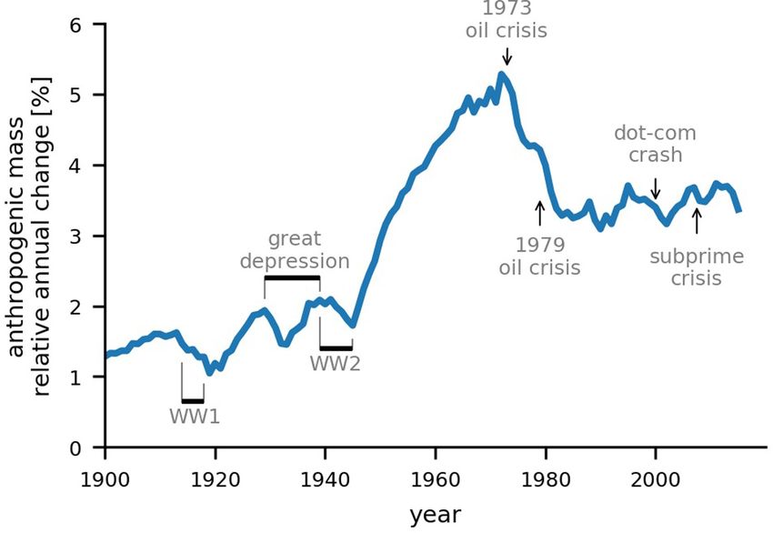
Article
                                                                               via TryDB69. For each species, the geometric mean dry matter content
Dynamic global vegetation models                                               value was calculated. Our best estimate of the leaves’ dry matter content
DGVM outputs were used in our plant biomass estimates throughout               was the geometric mean of all values. It was found to be 0.33 g/g, and
the studied period. For the years 1990–2017, the estimates were inte-          thus the wet-to-dry-mass conversion factor we used was 1/0.33 = 3.0.
grated with non-model estimates, as described above. The simulation               The three conversion factors were then multiplied by their corre-
outputs are part of the TRENDY v.8 project38,39, and followed the same         sponding compartment global dry mass11 to yield the global compart-
protocol, including both land-use and environmental (climate, CO2)             ment wet mass. Those were summed together to obtain the overall
time-varying effects (denoted as S3 in TRENDY; see ref. 39 and https://        global plant wet mass. We later combined the three factors to generate
sites.exeter.ac.uk/trendy for further details). The ensemble used here         a single integrated conversion factor, by dividing the global plant
comprised the following 15 models: CABLE-POP42, CLASS-CTEM43,                  wet mass by the dry mass. This integrated factor (2.0 g/g) was used
CLM5.044, DLEM45, ISAM46, JSBACH47, JULES-ES48, LPJ49, LPJ-GUESS50,            throughout this study to derive the overall biomass wet mass according
LPX-Bern51, OCN52, ORCHIDEE53, ORCHIDEE-CNP54, SDGVM55 and VISIT56.            to the dry mass. All steps from raw data to end result are documented
                                                                               in a Jupyter notebook at https://github.com/milo-lab/anthropogenic_
Anthropogenic mass and biomass extrapolation                                   mass/tree/master/wet_weight_calculation/wet_weight_calculation.
Extrapolation was used to estimate the time of intersection in Fig. 2          ipynb.
for the wet weight of biomass. To derive the future biomass change
(2018–2037), we used the linear rate of change calculated for 2010–2017,       Uncertainty estimation
and assumed that it would remain constant. The overall trend was found         Error propagation was performed using the Python Uncertainties
to be almost neutral given the uncertainty, as further discussed in Sup-       Package70. The carbon-to-dry-weight conversion factor was derived
plementary Information section 2. Anthropogenic mass estimates                 according to C content estimates obtained from different biomes (see
for future years (2015–2037) were extrapolated under an exponential            ‘Biomass C content estimation’ section). The overall uncertainty was
growth scenario. The exponent was derived on the basis of the most             found to be ±6%. The wet-to-dry conversion factor was calculated using
recent 5 years for which data were available22, under the simplified           values measured separately for roots, stems and leaves (see ‘Biomass
assumption that it would remain constant.                                      wet-weight estimation’ section). We found the total uncertainty of the
                                                                               dry-to-wet-weight conversion factor to be ±15%.
Biomass C content estimation                                                      The uncertainties of the years in which the anthropogenic mass
As part of the biomass calculation, we converted biomass on a                  and biomass intersect were estimated using Monte Carlo simu-
carbon-weight basis to a dry-weight basis by multiplying by a conver-          lations, with each parameter (for example, for dry biomass and
sion factor (2.25 g/g), which was calculated from estimates of the C           wet-to-dry-conversion-factor) randomly drawn according to its
content of different plant compartments (leaves, stems and roots) dif-         uncertainty range. The process was repeated 10,000 times, with the
ferentiated by biome57. For each biome, we calculated the average plant        resulting distribution dictating the overall uncertainty. All uncertain-
C content according to the mass fraction of each plant compartment58.          ties are reported as ±1 s.d. The anthropogenic mass uncertainties
Subsequently, the overall weighted plant C content was calculated on           used were based on corresponding estimates from ref. 22, assuming
the basis of the corresponding mass fraction of each biome10.                  a normal distribution. The uncertainties of the anthropogenic mass
   The total biomass C content conversion factor was then derived by           vary from ±2% to ±6% across the studied period. The waste uncertain-
computing the weighted average of the plant and non-plant factors,             ties range from ±4% in 1900 to ±7% in 2015. All calculation steps are
assuming that non-plant biomass represents 10% of total biomass                documented in a Jupyter notebook at https://github.com/milo-lab/
(based on ref. 11 and updates16,41). C content estimates for bacteria, which   anthropogenic_mass/tree/master/intersection_year_uncertainty/
represent the major contributor to non-plant biomass, were obtained            intersection_year_uncertainty.ipynb.
from refs. 59,60. All steps from raw data to end result are documented in         Following the biomass calculation (as described in the ‘Biomass
a Jupyter notebook available at https://github.com/milo-lab/anthro-            change over the years 1900–2017’ section), the total dry biomass
pogenic_mass/tree/master/C_content/biomass_C_content_estimation.               uncertainty was found to be ±16% for the years after 1990, and ±29%
ipynb.                                                                         for earlier years (±22% and ±33% for a wet-weight basis). The uncer-
                                                                               tainty was derived using the Python Uncertainties Package for the
Biomass wet-weight estimation                                                  plant component, Monte Carlo simulations for the non-plant com-
The biomass wet-weight was evaluated using a wet-to-dry-mass con-              ponent, and propagation70. All calculation steps are documented
version factor (Mwet/Mdry, the ratio between the wet and dry weights).         in a Jupyter notebook at https://github.com/milo-lab/anthropo-
The factor is composed of the corresponding factors of the main three          genic_mass/tree/master/biomass_calculation/biomass_uncertainty.
tree compartments: roots, stems and leaves.                                    ipynb.
   The roots’ conversion factor was calculated according to 30
wet-to-dry root mass measurements of four tree species61. Our best             Reporting summary
estimate for the conversion factor, 2.1 g/g, was the geometric mean            Further information on research design is available in the Nature
of all calculated conversion factors of all samples.                           Research Reporting Summary linked to this paper.
   The stems’ conversion factor was computed using a dataset of the
average green wood moisture content ((Mwet − Mdry)/Mdry) of 62 tree spe-
cies62. The dataset contains the moisture content values of sapwood and        Data availability
heartwood for each species. The best estimate of each species’ moisture        All data used in this study are available on GitHub, at https://
content value was based on the mean of the respective sapwood and              github.com/milo-lab/anthropogenic_mass. Anthropogenic mass
heartwood moisture content values (assuming a 1:1 mass ratio between           data are available from ref. 22 and at https://boku.ac.at/wiso/sec/
heartwood and sapwood). We then converted all moisture content                 data-download. TRENDY Dynamic Global Vegetation Models outputs
values to wet-to-dry-mass conversion factors. The geometric mean               are available at https://sites.exeter.ac.uk/trendy. Leaves dry matter
of the corresponding factors of all species was found to be 1.9 and was        content measurements were obtained via TryDB, at https://www.
used as our best estimate.                                                     try-db.org/. Other datasets used in this study are available from the
   The conversion factor of leaves was derived from dry matter con-            published literature, as detailed in the Methods and Supplementary
tent (Mdry/Mwet) datasets63–68, including 218 plant species, obtained          Information.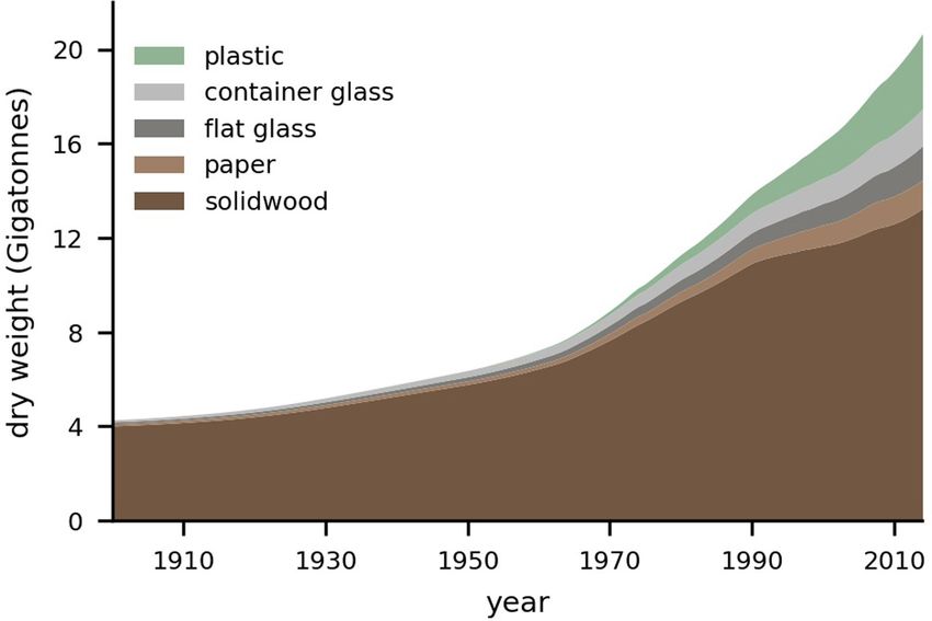
57.   Tang, Z. et al. Patterns of plant carbon, nitrogen, and phosphorus concentration in
Code availability                                                                                          relation to productivity in China’s terrestrial ecosystems. Proc. Natl Acad. Sci. USA 115,
                                                                                                           4033–4038 (2018).
All code used in this study is available on GitHub, at https://github.com/                           58.   Poorter, H. et al. Biomass allocation to leaves, stems and roots: meta-analyses of
milo-lab/anthropogenic_mass.                                                                               interspecific variation and environmental control. New Phytol. 193, 30–50 (2012).
                                                                                                     59.   Heldal, M., Norland, S. & Tumyr, O. X-ray microanalytic method for measurement of dry
                                                                                                           matter and elemental content of individual bacteria. Appl. Environ. Microbiol. 50,
33. Krausmann, F. et al. Economy-wide Material Flow Accounting. Introduction and Guide
                                                                                                           1251–1257 (1985).
    Version 1, Social Ecology Working Paper 151 (Alpen-Adria Univ., 2015).
                                                                                                     60.   von Stockar, U. & Liu, J. Does microbial life always feed on negative entropy?
34. Miatto, A., Schandl, H., Fishman, T. & Tanikawa, H. Global patterns and trends for
                                                                                                           Thermodynamic analysis of microbial growth. Biochim. Biophys. Acta 1412, 191–211 (1999).
    non-metallic minerals used for construction. J. Ind. Ecol. 21, 924–937 (2017).
                                                                                                     61.   Guo, L., Lin, H., Fan, B., Cui, X. & Chen, J. Impact of root water content on root biomass
35. Cooper, A. H., Brown, T. J., Price, S. J., Ford, J. R. & Waters, C. N. Humans are the most
                                                                                                           estimation using ground penetrating radar: evidence from forward simulations and field
    significant global geomorphological driving force of the 21st century. Anthropocene Rev.
                                                                                                           controlled experiments. Plant Soil 371, 503–520 (2013).
    5, 222–229 (2018).
                                                                                                     62.   Glass, S. V. & Zelinka, S. L. in Wood Handbook: Wood as an Engineering Material Vol. 190,
36. Food and Agriculture Organization of the United Nations. Global Forest Resources
                                                                                                           4.1–4.19 (US Department of Agriculture, 2010).
    Assessment 2010: Main Report (FAO, 2010).
                                                                                                     63.   Loveys, B. R. et al. Thermal acclimation of leaf and root respiration: an investigation
37. Liu, Y. Y. et al. Recent reversal in loss of global terrestrial biomass. Nat. Clim. Chang. 5,
                                                                                                           comparing inherently fast- and slow-growing plant species. Glob. Change Biol. 9,
    470–474 (2015).
                                                                                                           895–910 (2003).
38. Sitch, S. et al. Recent trends and drivers of regional sources and sinks of carbon dioxide.
                                                                                                     64.   Sheremetev, S. N. Herbs on the Soil Moisture Gradient (Water Relations and the
    Biogeosciences 12, 653–679 (2015).
                                                                                                           Structural-Functional Organization) (KMK, 2005).
39. Friedlingstein, P. et al. Global carbon budget 2019. Earth Syst. Sci. Data 11, 1783–1838
                                                                                                     65.   Michaletz, S. T. & Johnson, E. A. A heat transfer model of crown scorch in forest fires. Can.
    (2019).
                                                                                                           J. For. Res. 36, 2839–2851 (2006).
40. Food and Agriculture Organization of the United Nations FAOSTAT http://faostat.fao.org.
                                                                                                     66.   Messier, J., McGill, B. J. & Lechowicz, M. J. How do traits vary across ecological scales? A
41. Magnabosco, C. et al. The biomass and biodiversity of the continental subsurface. Nat.
                                                                                                           case for trait-based ecology. Ecol. Lett. 13, 838–848 (2010).
    Geosci. 11, 707–717 (2018).
                                                                                                     67.   Boucher, F. C., Thuiller, W., Arnoldi, C., Albert, C. H. & Lavergne, S. Unravelling the
42. Haverd, V. et al. A new version of the CABLE land surface model (Subversion revision
                                                                                                           architecture of functional variability in wild populations of Polygonum viviparum L. Funct.
    r4601) incorporating land use and land cover change, woody vegetation demography,
                                                                                                           Ecol. 27, 382–391 (2013).
    and a novel optimisation-based approach to plant coordination of photosynthesis.
                                                                                                     68.   Dahlin, K. M., Asner, G. P. & Field, C. B. Environmental and community controls on plant
    Geosci. Model Dev. 11, 2995–3026 (2018).
                                                                                                           canopy chemistry in a Mediterranean-type ecosystem. Proc. Natl Acad. Sci. USA 110,
43. Melton, J. R. & Arora, V. K. Competition between plant functional types in the Canadian
                                                                                                           6895–6900 (2013).
    Terrestrial Ecosystem Model (CTEM) v. 2.0. Geosci. Model Dev. 9, 323–361 (2016).
                                                                                                     69.   Kattge, J. et al. TRY–a global database of plant traits. Glob. Change Biol. 17, 2905–2935
44. Lawrence, D. M. et al. The community land model version 5: description of new features,
                                                                                                           (2011).
    benchmarking, and impact of forcing uncertainty. J. Adv. Model. Earth Syst. 11, 4245–4287
                                                                                                     70.   Lebigot, E. O. Uncertainties: a Python package for calculations with uncertainties. https://
    (2019).
                                                                                                           pythonhosted.org/uncertainties/ (2010).
45. Tian, H. et al. North American terrestrial CO2 uptake largely offset by CH4 and N2O
                                                                                                     71.   Wiedenhofer, D., Fishman, T., Lauk, C., Haas, W. & Krausmann, F. Integrating material stock
    emissions: toward a full accounting of the greenhouse gas budget. Clim. Change 129,
                                                                                                           dynamics into economy-wide material flow accounting: concepts, modelling, and global
    413–426 (2015).
                                                                                                           application for 1900–2050. Ecol. Econ. 156, 121–133 (2019).
46. Meiyappan, P., Jain, A. K. & House, J. I. Increased influence of nitrogen limitation on CO2
    emissions from future land use and land use change. Glob. Biogeochem. Cycles 29,
    1524–1548 (2015).                                                                                Acknowledgements We thank U. Alon, S. Dan, G. Eshel, T. Fishman, E. Gelbrieth, T. Kaufmann,
47. Mauritsen, T. et al. Developments in the MPI-M Earth System Model version1.2                     T. Klein, A. Knoll, E. Noor, N. Page, R. Phillips, J. Pongratz, M. Shamir, M. Shtein, B. Smith,
    (MPI-ESM1.2) and its response to increasing CO2. J. Adv. Model. Earth Syst. 11, 998–1038         C. Waters, T. Wiesel, M. Williams and members of our laboratory for help and discussions,
    (2019).                                                                                          and S. Sitch and the TRENDY DGVM community for access to their simulation outputs. This
48. Clark, D. B. et al. The Joint UK Land Environment Simulator (JULES), model description –         research was supported by the European Research Council (Project NOVCARBFIX 646827);
    Part 2: Carbon fluxes and vegetation dynamics. Geosci. Model Dev. 4, 701–722 (2011).             Beck-Canadian Center for Alternative Energy Research; Dana and Yossie Hollander; Ullmann
49. Poulter, B., Frank, D. C., Hodson, E. L. & Zimmermann, N. E. Impacts of land cover and           Family Foundation; Helmsley Charitable Foundation; Larson Charitable Foundation; Wolfson
    climate data selection on understanding terrestrial carbon dynamics and the CO2                  Family Charitable Trust; Charles Rothschild; and Selmo Nussenbaum. R.M. is the Charles and
    airborne fraction. Biogeosciences 8, 2027–2036 (2011).                                           Louise Gartner professional chair. Y.M.B.-O is an Azrieli Fellow.
50. Smith, B. et al. Implications of incorporating N cycling and N limitations on primary
    production in an individual-based dynamic vegetation model. Biogeosciences 11,
    2027–2054 (2014).                                                                                Author contributions E.E., L.B.-U. and R.M. wrote the manuscript. E.E. performed the bulk of
51. Lienert, S. & Joos, F. A Bayesian ensemble data assimilation to constrain model                  the research and data analysis. L.B.-U. contributed to the anthropogenic mass analysis and
    parameters and land-use carbon emissions. Biogeosciences 15, 2909–2930 (2018).                   biomass estimation. Y.M.B.-O. contributed to the biomass estimation and carbon content
52. Zaehle, S. & Friend, A. D. Carbon and nitrogen cycle dynamics in the O-CN land surface           calculation. J.G. contributed to the water content calculation. E.E., J.G. and Y.M.B.-O.
    model: 1. Model description, site-scale evaluation, and sensitivity to parameter estimates.      performed the uncertainty analysis. E.E., L.B.-U. and R.M. conceived the study. R.M. supervised
    Glob. Biogeochem. Cycles 24, GB1005 (2010).                                                      the study. All authors discussed the results, and commented on the manuscript.
53. Krinner, G. et al. A dynamic global vegetation model for studies of the coupled
    atmosphere–biosphere system. Glob. Biogeochem. Cycles 19, GB1015 (2005).                         Competing interests The authors declare no competing interests.
54. Goll, D. S. et al. Carbon–nitrogen interactions in idealized simulations with JSBACH
    (version 3.10). Geosci. Model Dev. 10, 2009–2030 (2017).                                         Additional information
55. Walker, A. P. et al. The impact of alternative trait-scaling hypotheses for the maximum          Supplementary information is available for this paper at https://doi.org/10.1038/s41586-020-
    photosynthetic carboxylation rate (Vcmax) on global gross primary production. New Phytol.        3010-5.
    215, 1370–1386 (2017).                                                                           Correspondence and requests for materials should be addressed to R.M.
56. Kato, E., Kinoshita, T., Ito, A., Kawamiya, M. & Yamagata, Y. Evaluation of spatially explicit   Peer review information Nature thanks Fridolin Krausmann, Dominik Wiedenhofer and the
    emission scenario of land-use change and biomass burning using a process-based                   other, anonymous, reviewer(s) for their contribution to the peer review of this work.
    biogeochemical model. J. Land Use Sci. 8, 104–122 (2013).                                        Reprints and permissions information is available at http://www.nature.com/reprints.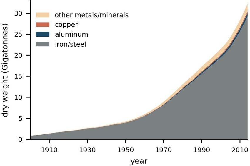
Article

Extended Data Fig. 1 | Sensitivity analysis of the anthropogenic mass              roundwood. The total biomass weight is depicted by the green line. Black dot
definition. a–f, The effect of adding the following to the anthropogenic mass      indicates the year of intersection based on the alternative anthropogenic mass
(dark purple): a, mass of the human population, b, mass of livestock, c, mass of   definition. Violet area and light green-dashed line indicate extrapolated
crops and agroforestry, d, mass of earthworks, dredging and waste/                 anthropogenic mass and biomass estimates, respectively. Full description of
overburden from mineral and metal production, and f, mass of anthropogenic         the sensitivity analysis is provided in Supplementary Information section 1.
atmospheric CO2 stocks, as well as e, the exclusion of the mass of industrial
Extended Data Fig. 2 | Anthropogenic mass composition since the year 1900, divided into material groups. Dataset is based on ref. 22.
Article

Extended Data Fig. 3 | Anthropogenic mass relative annual change, with
highlights of notable global events. Relative annual change is calculated as
the difference between two consecutive years divided by the earlier year
anthropogenic mass value.
Extended Data Fig. 4 | Anthropogenic mass metal estimates since the
beginning of the twentieth century, divided into material sub-groups. Data
are taken from the comprehensive work of the Institute of Social Ecology,
Vienna. We used a recent study71, which has some minor updates compared to
the study used to achieve the main results22.
Article

Extended Data Fig. 5 | Anthropogenic mass estimates for (industrial round)
wood, glass and plastic since the beginning of the twentieth century,
divided into material sub-groups. Data are taken from the comprehensive
work of the Institute of Social Ecology, Vienna. We used a recent study71, which
has some minor updates compared to the study used to achieve the main
results22.
Extended Data Fig. 6 | Calculation steps in plant biomass estimation for 1990–2017. As further detailed in the Methods section ‘Biomass change over the years
1900–2017’.
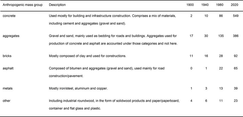
Article
Extended Data Table 1 | The different anthropogenic mass groups and their mass estimates in selected years

The mass values are presented in gigatonnes (Gt; 1,000 Gt = 1 Tt). The 2020 estimate is partially extrapolated (since 2016). Overall, the categories of anthropogenic mass presented give almost
complete coverage of materials usage (>98% in terms of mass based on ref. 21).
nature research | reporting summary
                                                                                                      Corresponding author(s): Ron Milo
                                                                                                      Last updated by author(s): Sep 5, 2020

Reporting Summary
Nature Research wishes to improve the reproducibility of the work that we publish. This form provides structure for consistency and transparency
in reporting. For further information on Nature Research policies, see Authors & Referees and the Editorial Policy Checklist.

Statistics
For all statistical analyses, confirm that the following items are present in the figure legend, table legend, main text, or Methods section.
n/a Confirmed
           The exact sample size (n) for each experimental group/condition, given as a discrete number and unit of measurement
           A statement on whether measurements were taken from distinct samples or whether the same sample was measured repeatedly
           The statistical test(s) used AND whether they are one- or two-sided
           Only common tests should be described solely by name; describe more complex techniques in the Methods section.

           A description of all covariates tested
           A description of any assumptions or corrections, such as tests of normality and adjustment for multiple comparisons
           A full description of the statistical parameters including central tendency (e.g. means) or other basic estimates (e.g. regression coefficient)
           AND variation (e.g. standard deviation) or associated estimates of uncertainty (e.g. confidence intervals)

           For null hypothesis testing, the test statistic (e.g. F, t, r) with confidence intervals, effect sizes, degrees of freedom and P value noted
           Give P values as exact values whenever suitable.

           For Bayesian analysis, information on the choice of priors and Markov chain Monte Carlo settings
           For hierarchical and complex designs, identification of the appropriate level for tests and full reporting of outcomes
           Estimates of effect sizes (e.g. Cohen's d, Pearson's r), indicating how they were calculated
                                                 Our web collection on statistics for biologists contains articles on many of the points above.

Software and code
Policy information about availability of computer code
  Data collection              All code used in this study is available on GitHub, at https://github.com/milo-lab/anthropogenic_mass.

  Data analysis                All code used in this study is available on GitHub, at https://github.com/milo-lab/anthropogenic_mass.
For manuscripts utilizing custom algorithms or software that are central to the research but not yet described in published literature, software must be made available to editors/reviewers.
We strongly encourage code deposition in a community repository (e.g. GitHub). See the Nature Research guidelines for submitting code & software for further information.

Data
Policy information about availability of data
 All manuscripts must include a data availability statement. This statement should provide the following information, where applicable:
     - Accession codes, unique identifiers, or web links for publicly available datasets
     - A list of figures that have associated raw data
     - A description of any restrictions on data availability

All data used in this study are available on GitHub, at https://github.com/milo-lab/anthropogenic_mass. Anthropogenic mass data is available from ref. 22 and at:
https://boku.ac.at/wiso/sec/data-download. TRENDY Dynamic Global Vegetation Models outputs are available at: https://sites.exeter.ac.uk/trendy. Leaves dry
                                                                                                                                                                                                October 2018

matter content measurements were obtained via TryDB, at: https://www.try-db.org/. Other datasets used in this study are available from published literature, as
detailed in the Methods section and Supplementary Information.

                                                                                                                                                                                                      1
nature research | reporting summary
Field-specific reporting
Please select the one below that is the best fit for your research. If you are not sure, read the appropriate sections before making your selection.
Life sciences Behavioural & social sciences Ecological, evolutionary & environmental sciences
For a reference copy of the document with all sections, see nature.com/documents/nr-reporting-summary-flat.pdf
Ecological, evolutionary & environmental sciences study design
All studies must disclose on these points even when the disclosure is negative.
Study description Quantitative comparison of the global living biomass and human-made mass, since the beginning of the 20th century.
Research sample Human-made mass data, divided into material sub-groups and living biomass data.
Sampling strategy All relevant data were used. No statistical methods were used to predetermine sample size.
Data collection Data was based on existing datasets and was collected online by the authors.
Timing and spatial scale Global data since 1900, consistent with the time period and global scope of the study.
Data exclusions No data were excluded from the analyses.
Reproducibility This is not an experimental study, thus experimental replication was not performed. The analysis is reproducible given the code
provided, which includes all steps from raw data to end results.
Randomization All living organisms were grouped into one group, all human-made masses were grouped into another group.
Blinding Not relevant, since this study is not experimental.
Did the study involve field work? Yes No
Reporting for specific materials, systems and methods
We require information from authors about some types of materials, experimental systems and methods used in many studies. Here, indicate whether each material,
system or method listed is relevant to your study. If you are not sure if a list item applies to your research, read the appropriate section before selecting a response.
Materials & experimental systems Methods
n/a Involved in the study n/a Involved in the study
Antibodies ChIP-seq
Eukaryotic cell lines Flow cytometry
Palaeontology MRI-based neuroimaging
Animals and other organisms
Human research participants
Clinical data
October 2018
2You can also read