Extreme Values of Wind Speed over the Kara Sea Based on the ERA5 Dataset
←
→
Page content transcription
If your browser does not render page correctly, please read the page content below
Atmospheric and Climate Sciences, 2021, 11, 98-113
                                                                                               https://www.scirp.org/journal/acs
                                                                                                          ISSN Online: 2160-0422
                                                                                                            ISSN Print: 2160-0414

Extreme Values of Wind Speed over the Kara
Sea Based on the ERA5 Dataset

Alexander Kislov1, Tatyana Matveeva2

Department of Meteorology and Climatology, Faculty of Geography, Lomonosov Moscow State University, Moscow, Russia
1

Laboratory of Climate, Institute of Geography, Russian Academy of Sciences, Moscow, Russia
2

How to cite this paper: Kislov, A. and          Abstract
Matveeva, T. (2021) Extreme Values of
Wind Speed over the Kara Sea Based on the       Extreme values of wind speed were studied based on the highly detailed ERA5
ERA5 Dataset. Atmospheric and Climate           dataset covering the central part of the Kara Sea. Cases in which the ice cov-
Sciences, 11, 98-113.                           erage of the cells exceeded 15% were filtered. Our study shows that the wind
https://doi.org/10.4236/acs.2021.111007
                                                speed extrema obtained from station observations, as well as from modelling
Received: October 26, 2020                      results in the framework of mesoscale models, can be divided into two groups
Accepted: January 1, 2021                       according to their probability distribution laws. One group is specifically des-
Published: January 4, 2021                      ignated as black swans, with the other referred to as dragons (or dragon-kings).
Copyright © 2021 by author(s) and
                                                In this study we determined that the data of ERA5 accurately described the
Scientific Research Publishing Inc.             swans, but did not fully reproduce extrema related to the dragons; these ex-
This work is licensed under the Creative        trema were identified only in half of ERA5 grid points. Weibull probability
Commons Attribution International               distribution function (PDF) parameters were identified in only a quarter of
License (CC BY 4.0).
                                                the pixels. The parameters were connected almost deterministically. This
http://creativecommons.org/licenses/by/4.0/
               Open Access
                                                converted the Weibull function into a one-parameter dependence. It was not
                                                clear whether this uniqueness was a consequence of the features of the calcu-
                                                lation algorithm used in ERA5, or whether it was a consequence of a rela-
                                                tively small area being considered, which had the same wind regime. Ex-
                                                tremes of wind speed arise as mesoscale features and are associated with hy-
                                                drodynamic features of the wind flow. If the flow was non-geostrophic and if
                                                its trajectory had a substantial curvature, then the extreme velocities were
                                                distributed according to a rule similar to the Weibull law.

                                                Keywords
                                                ERA5, Kara Sea, Weibull Probability Distribution Function Wind Speed,
                                                Hydrodynamics and Statistics of Extreme Events

                                              1. Introduction
                                              A large part of the Kara Sea (Figure 1) is covered with ice year-round. From the

DOI: 10.4236/acs.2021.111007 Jan. 4, 2021                          98                           Atmospheric and Climate Sciences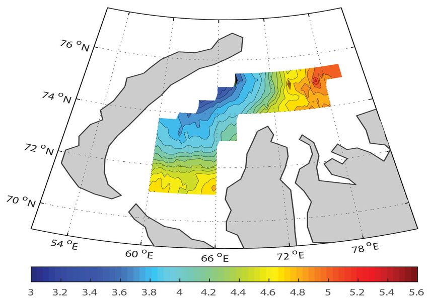
A. Kislov, T. Matveeva
point of view of temperature, roughness, and other characteristics, this means
that the surface of the sea merges with the land. In the warm season, the ice
breaks up into separate massifs and the features of the marine surface are mani-
fested in the meteorological regime. The purpose of this article is to study ex-
treme winds above the marine surface when the area of ice covering each grid
cell of ERA5 was less than 15%. At this time of year, an especially strong wind
over the Kara Sea is associated with cyclones that make landfall from the west
and southwest, and sometimes regenerate over the Kara Sea [1].
The Arctic region is characterized by sparse in-situ observational coverage
(conventional coastal weather stations, buoys, ships). Exceedingly few studies
(e.g., [2] [3] [4] [5]) have examined climatological Arctic winds from station ob-
servations located in the sea-shore zone. Most marine surface wind speed data
are provided by satellite sensors (scatterometer, microwave radiometer, altime-
ter, and synthetic aperture radar) (e.g., [6] [7] [8] [9]). However, sea ice limits
satellite use in the Arctic [10], restricting the poleward coverage of the satel-
lite-based characterizations. For example, scatterometer data does not exist for
most of the Arctic.
Reanalysis data provide a useful alternative for filling these gaps in wind speed
data over the Arctic, as they have global coverage and combine weather forecast
models and assimilation of observations from a wide variety of sources. Model-
ling data (for example, within the framework of the historical CMIP5 experi-
ment) have also been used to assess the pattern of surface wind climatology.
The climatology of winds across the oceans is detailed in multiple works [11]
[12] [13], and wind regime information for the Arctic is highlighted in several
studies [14] [15]. Regional climatology of near surface winds includes informa-
tion over Alaska and the adjacent Arctic Ocean [16] [17], over several sectors of
Canada [2], over the seas of European and Siberian sectors of Arctic [1] [4], over
the northeast Pacific Ocean [5] and so on.
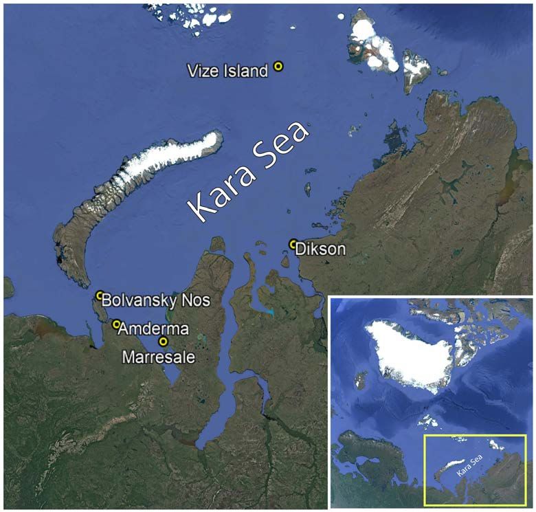
Figure 1. The Kara Sea and locations of observation stations, which were used for
ERA5-data comparison. Bottom right insert: map of the Arctic. A yellow frame marks the
area for the main map. (Image source: https://www.google.com/maps).
DOI: 10.4236/acs.2021.111007 99 Atmospheric and Climate Sciences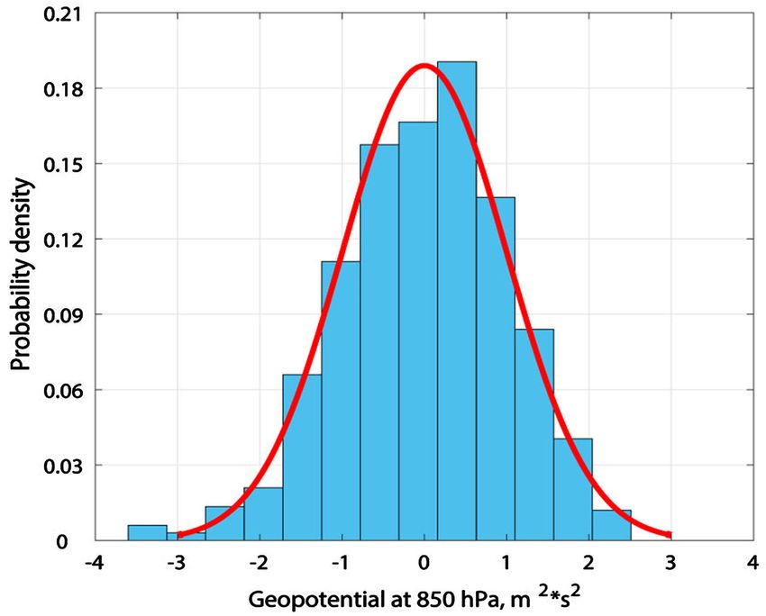
A. Kislov, T. Matveeva

                                  This study focuses on the Kara Sea, a small part of the Pan-Arctic domain, to
                               more clearly delineate its regional characteristics. For this purpose, a horizon-
                               tally detailed re-analysis of ERA5 was used. This product (see below) was devel-
                               oped by the European Centre for Medium-Range Weather Forecasts (ECMWF).
                               There is relatively little research that has been published on the climate of this
                               region. Additionally, we consider the issues of hydrodynamic substantiation in
                               evaluating the peculiarity of extreme value statistical laws.
                                  The Weibull distribution has traditionally been used for statistical approxima-
                               tions of wind extremes [4] [11] [18]. The data selected for extreme value analysis
                               must be identically distributed and independent. However, the methods could be
                               used for dependent time series [19] [20]. For an identical distribution, our
                               analysis demonstrated that each set of wind speed extremes (observed in both
                               coastal and open-ocean locations) is a mixture of two different subsets, with each
                               neatly described by the Weibull distribution. The volumes of these subsets are
                               not the same. Almost all samples belong to the so-called base distribution, and
                               only a few percent (or less) of the samples (mostly strong events) are described
                               by another Weibull distribution. Representatives of the base population were
                               marked as swans (and black swans in their upper limit) and representatives of
                               the other group were identified as dragons. This terminology was introduced in
                               several studies [21] [22] [23] [24]. We do not follow these researchers’ specifica-
                               tions regarding the details of specific origins of events, their predictability, and
                               so on, and instead use the terms only to mark the differences of samples belong-
                               ing to various groups.
                                  Apart from the statistical approach, an explanation of the observed wind
                               speed probability distribution should be based on theoretical ideas from hydro-
                               dynamic peculiarities of the atmospheric motion. This justification can be ob-
                               tained by studying the products of numerical simulations or by studying equa-
                               tions that are sufficiently simplified to obtain their analytical solutions. In a pre-
                               vious paper, we concluded that the wind extremes modelled by a general circula-
                               tion model involved only samples conforming to the base distribution (swans).
                               The same conclusion was derived after reanalysing the ERA Interim dataset.
                               Thus, the numerical coarse resolution products did not contain observed excep-
                               tional outliers.
                                  The next step of our analysis was to investigate how accurately a mesoscale
                               atmospheric model (with a fine spatial resolution) simulated the aforementioned
                               peculiarities of wind extremes [5] [25]. We observed that an atmospheric model
                               with a detailed resolution (in this study, we used the data from a domain with a
                               13.2 km spatial resolution) did simulate the largest wind speed extremes. Un-
                               fortunately, a more thorough analysis showed that the differences in the pa-
                               rameters of the PDFs were still substantial.
                                 In this study, we continue the investigation of the ability of numerical simula-
                               tions to reproduce wind speed extremes based on the ERA5 dataset [26] [27]
                               [28] also used this approach for multiple simulation types, and ERA5 was
                               marked as the most accurate of the studied group. In [29], the ERA5 surface

DOI: 10.4236/acs.2021.111007                        100                             Atmospheric and Climate Sciences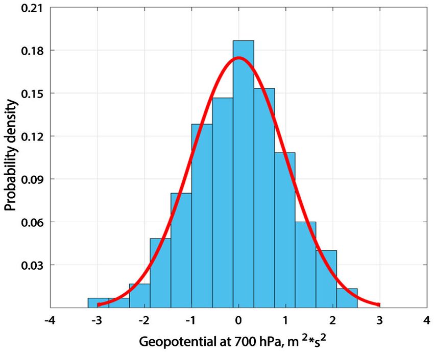
A. Kislov, T. Matveeva

                               wind data were compared with Advanced Scatterometer (ASCAT) data, and a
                               strong accordance was observed.
                                  Regarding analytical models, several studies (e.g., [30] [31]) have noted that a
                               Rayleigh distribution (a special case of the Weibull distribution) emerges for the
                               wind speed if the vector wind components are assumed to be individually Gaus-
                               sian. To obtain a physical understanding of the observed PDFs of sea surface
                               wind speeds, a stochastic model for boundary layer winds (including several as-
                               sumptions and parameterizations) was developed [11]. In our study, we consid-
                               ered another simple hydrodynamics model where a Weibull-like distribution
                               naturally arises for the wind speed anomaly distribution.
                                  In the next section, we describe the data and study area, and briefly summa-
                               rize the methods. Section 3 describes the evidence for a Weibull distribution in
                               the near surface wind speed. Section 4 is devoted to explaining how the Weibull
                               distribution arises from simplified equations of hydrodynamics. Section 5 con-
                               cludes the paper.

                               2. Data and Methods
                               In this study, we used the new global reanalysis ERA5 developed by the
                               ECMWF. The ERA5 reanalysis was improved compared to a previous successful
                               ERA-Interim reanalysis [26]. Specifically, the horizontal resolution was im-
                               proved to 0.25˚ × 0.25˚, the number of vertical levels was increased to 137 pres-
                               sure levels from 1000 hPa to 1 hPa, the temporal resolution was changed to
                               hourly, and the list of output parameters was extended. Furthermore, the num-
                               ber of assimilated observations was enhanced (approximately five times more
                               compared to ERA-Interim) [27]. Most of the ERA-Interim problems with re-
                               processing of satellite data were solved and the system of assimilation was im-
                               proved in ERA5.
                                  For our purposes, we used zonal and meridional components of wind speed at
                               10 meters, the geopotential at 700 hPa and 850 hPa, and the sea ice concentra-
                               tion.
                                  To apply statistical approaches, we composed our data according to the inde-
                               pendence condition. Practically, this means that the data sample had to include
                               only independent extreme values. We selected the maximum wind speeds from
                               3-day intervals in wind speed data for each grid cell. This interval was obtained
                               via autocorrelation function analysis as a period for the disappearance of the
                               correlation between fluctuations (correlation coefficient becomes insignificant).
                               The same time intervals for the same aims were used in several previous studies
                               [4] [32] [33].
                                  During the summer, Kara Sea may either be open water or covered with ice of
                               various concentrations. This causes different roughness conditions, as the
                               roughness of open water is usually lower than that of sea ice. Drag coefficients
                               for open water are approximately 1.5 - 2 times lower than compared to the sea
                               ice surface [34]. Our samples were thus divided into sea ice and open water con-
                               ditions, because in some regions, the share of days with ice cover reached 40% -

DOI: 10.4236/acs.2021.111007                        101                           Atmospheric and Climate Sciences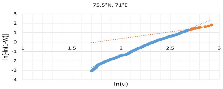
A. Kislov, T. Matveeva
50%. As a criterion for this division, we used the concentration threshold of 15%
(involving in ERA5). The days with a sea ice concentration higher than 15%
were considered as sea ice conditions and lower than 15% meant open water. We
compared statistical results for both open water events and sea ice conditions
(see below). In our analysis, we used only open water samples.
3. Statistical Features of the Observed Sea Surface Wind
Speed
As mentioned, the statistics for extreme wind speed were described by the
Weibull distribution. The following equations represent the cumulative distribu-
tion function (W, CDF) and the PDF (w):
u k
W (u ) =
1 − exp − (1a)
V
ku k −1 u k
w (u )
= exp − (1b)
Vk V
The value of V determines the scale of speed. A value of u = V corresponds
to W ( u ) = 0.63 . This means that V is slightly more than the median ( umed ), and
( ln 2 )
−1 k
V = umed . The dependence of moments of the distribution on the
Weibull parameters is illustrated in Monahan (2006a). Note that the Weibull
distribution for k = 3.6 approximates a Normal distribution within a range ex-
tended to several values of standard deviation.
The Weibull parameters (k, V) are estimated using the maximum likelihood
method. One variant of this method is discussed in [4]. In Figure 2, several
“Weibull Plots” are shown as calculated based on the ERA5 data, where a
straight line is recovered if the sample shows a Weibull distribution. The quality
of description we can see visually and quantitatively based on the coefficient of
determination (R2) providing a measure of the success of approximation. At all
sites of the Kara Sea, we observed that practically all points of the CDF (besides
several points depicting rare and high speeds) showed a close approximation to a
Weibull distribution. In a mathematical sense, the use of R2 is related to the ap-
plication of the Cramer-Mises-Smirnov statistical criterion. The application of
the Kolmogorov-Smirnov test also showed that there was no reason not to trust
the Weibull distribution (see, for example, [4]).
Thus, most events fit into the basic distribution, and some of the most pow-
erful ones did not fall into it. This result falls under the classification introduced
in the Introduction, i.e., when the sample data of the same item refers to differ-
ent distribution functions. In ERA5, the swans (and black swans) are always
represented. Unlike station data, dragons are completely absent in some pixels
(Figure 2(a) and Figure 2(b)). This repeats what we observed in results of the
general circulation model with a coarse resolution [4] [5]. In other points, they
were represented by only a few anomalies that decidedly did not fall within the
basic distribution, and it was impossible to estimate distribution parameters
DOI: 10.4236/acs.2021.111007 102 Atmospheric and Climate Sciences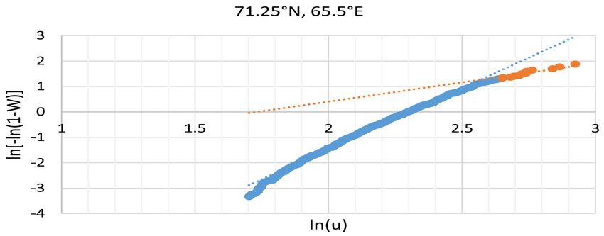
A. Kislov, T. Matveeva

                                     (a)

                                     (b)

                                     (c)

                                     (d)

                                     (e)

DOI: 10.4236/acs.2021.111007   103         Atmospheric and Climate Sciences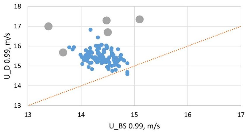
A. Kislov, T. Matveeva

                                                                           (f)

                               Figure 2. Cumulative distribution functions of wind speed maxima (ERA5) for 72 hours
                               time step records straightening on the coordinate axis of the Weibull distribution, and li-
                               near regression line corresponding to the Weibull function. Examples for different ERA5
                               grid points ((a)-(f)).

                               from such a small volume of samples (Figure 2(c)). In some pixels, a sufficient
                               number of linearly spaced points dropped out of the base distribution, which
                               emphasized their commonality and belonging to the same distribution law
                               (Figures 2(d)-(f)). Therefore, we considered (based on statistical criteria) that
                               the estimation of the distribution parameters was acceptable. As a result, said es-
                               timation was implemented for 126 pixels (out of 520 covering the studied area).
                                  As a rule, with respect to a certain group of points, it is impossible to deter-
                               mine the population that they belong to, as the trend lines on the graphs practi-
                               cally coincide (Figure 2). In this case, we attributed them both to the swans and
                               dragons.
                                  In the basic distribution, the values of V and k were unique in different pixels,
                               but V varied minimally, i.e., from 9.5 to 10.5 m/s. Changes in the exponent were
                               much more substantial (from 3 to 5). The parameter k increased in the south
                               and east directions of the region, adjacent to Novaya Zemlya (Figure 3). In the
                               central part of the Kara Sea, k was close to 3.6. Here, the probability distribution
                               was close to Gaussian. Further south and east, the k increased and the tail of the
                               PDF became lighter than that of the Gaussian distribution, which meant that the
                               probability of strong winds continuously lessened until unrealistically small val-
                               ues were reached. However, this conclusion will fundamentally change when the
                               presence of dragons is considered. Therefore, we can conclude that the geo-
                               graphical features of the PDFs were determined by changes in the exponent.
                               Having expressed the moments of distribution through V and k [11], we ob-
                               served that the skewness was near zero (from −0.2 to +0.2), and the kurtosis
                               varied from −0.03 to −0.3.
                                  For dragons, the exponent in the Weibull distribution was substantially less
                               than for swans (the value of k varied from 1 to 3). This meant that the distribu-
                               tion differed from the normal distribution because of the presence of a heavier
                               tail, and that the likelihood of strong winds increased.
                                  In Figure 4, all results are summarized in the parameter field (k, V). Each
                               population had its own range of values, and a clear connection of parameters
                               was present.

DOI: 10.4236/acs.2021.111007                          104                              Atmospheric and Climate Sciences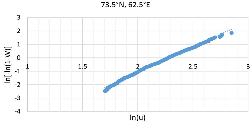
A. Kislov, T. Matveeva

                                                Figure 3. Spatial distribution of the Weibull parameter k.

                                Figure 4. The Weibull distribution parameters (k and V) calculated for all pixels of the
                                ERA5 (covering central part of the Kara Sea—see Figure 3), S er5_K and D er5_K for
                                swans and dragons, respectively, and additionally, data from stations located around the
                                Kara Sea (see Figure 1), S st_K and D st_K for swans and dragons, respectively.

                                                                                                  =
                                  The expression for the basic range, i.e., the swans, was given by V 0.36k + 8.7
                                with a low coefficient of determination. As V varied minimally compared to the
                                variations of k, and there was thus no reason to expect a correlation. For drag-
                               ons, V 5.62 ln ( k ) + 3.29 , R 2 = 0.99 . A close relationship between the pa-
                               =
                                rameters meant that the Weibull distribution encompassed a single parameter.
                                   The reason for this unambiguity was unclear; it may have been a consequence
                                of the algorithm for calculating the wind speed near the sea surface in the ERA5
                                reanalysis. Alternately, this may have occurred because we examined a relatively
                                small area, as it contained a uniform wind regime. A comparison of the parame-
                                ters (k, V) according to station measurements in the Arctic does not demon-
                                strate such a close relationship. There was an increase in V with increasing k.
                                Existence of a strong connection between V and k was not noted according to
                                the scatterometer [11].
                                   Figure 4 includes similar data on measurements at five stations located in the
                                coastal zone of the Kara Sea: Bolvansky Nos (70.5˚N, 59.1˚E), Amderma
                                (69.8˚N, 61.7˚E), Marresale (69.7˚N, 66.8˚E), Vize Island (79.5˚N, 77.0˚E), and
                                Dikson (73.5˚N, 80.2˚E) [4]. These data are in accordance with the reanalysis
                                data, thus emphasizing its high quality.
                                  Even though anomalies related to dragons are rare events, their presence or
                                absence are unprincipled for the parameters of the basic distribution, and ne-
                                glecting them can lead to an incorrect interpretation of the results. To illustrate,
                                consider the situation at pixel 71.5˚N, 60˚E. In this cell, there were 26 events re-

DOI: 10.4236/acs.2021.111007                          105                              Atmospheric and Climate Sciences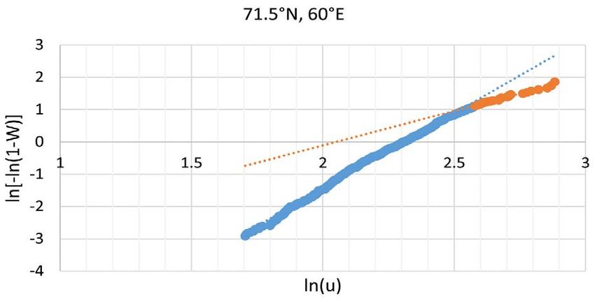
A. Kislov, T. Matveeva

                               lated to “dragons” (with respect to 20 events, it was impossible to make a con-
                               clusion about which affiliation, i.e., dragons or black swans, that they belonged
                               to) (Figure 2(d)). The Weibull distribution parameters were k = 4.66 and V =
                               10.1 m/s for swans, and k = 2.14 and V = 7.8 m/s for dragons. If we estimate the
                               average u and the variance D from the base distribution (using well-known
                               formulas: u = V Γ (1 + 1 k ) , D = V 2 Γ (1 + 2 k ) − u 2 , Γ is the gamma function),
                               we obtain u = 9.2 m s и D = 6.15 m 2 s 2 . If at this point the sample is not di-
                               vided into swans and dragons, then k = 4.46 and V = 10.2 m/s and и
                                u = 9.3 m s и D = 6.1 m 2 s 2 . The distribution moments are almost identical
                               in the two examples; however, without isolating the dragon population, the larg-
                               est anomalies are outside the scope of statistical analysis. Accordingly, the quan-
                               tile value corresponding to a probability of 0.99, as calculated from the base dis-
                                                    V [ − ln 0.01] =
                                                                   1k
                               tribution, was u0.99 =               14 m s . According to the distribution of
                               dragons, we then obtain u0.99 = 16 m s . Naturally, this result demonstrates that
                               in reality extrema occur much more often than is prescribed by the basic distri-
                               bution.
                                 Figure 5 compares pairs of quantile values for the pixels in which, in addition
                               to swans, it was possible to identify dragons and evaluate the parameters of their
                               distribution. Similar data on station measurements are given here; interestingly,
                               u0.99 was larger for dragons. Station data were characterized by large differences
                               between representatives of different populations. This result, together with the
                               already noted situation that the statistical properties of dragons were evaluated
                               only in a quarter of cases, suggested that the ERA5 did not fully provide infor-
                               mation on the largest extremes. We encountered the same phenomenon when
                               analysing COSMO-CLM data with a horizontal step of 13.2 km: The model re-
                               produced dragons, but they were not as powerful as those obtained from the
                               measurement data [5].
                                 Consider what happens if the selection of information (on the grounds of a
                               lack of ice cover) is not carried out. The calculations showed, first, that with ice,
                               the wind speed distribution was described by the Weibull distribution with a
                               high accuracy (the determination coefficients never fell below 0.95). Second,

                               Figure 5. Quantile wind speed values U (0.99) in m/s for wind data from ERA5 calculated
                               separately for two groups of wind speed extremes come from the black swans and dra-
                               gons populations, and additionally, data from stations located around the Kara Sea (see
                               Figure 1).

DOI: 10.4236/acs.2021.111007                         106                            Atmospheric and Climate Sciences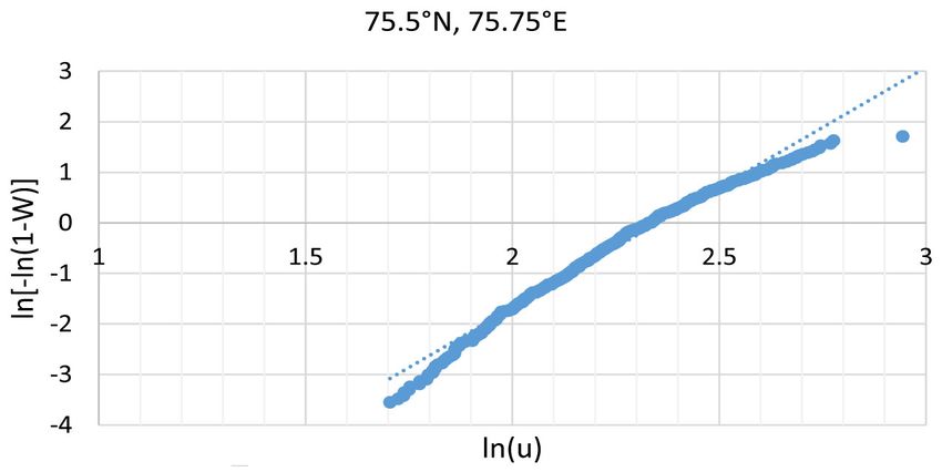
A. Kislov, T. Matveeva

                               dragons were almost completely absent in the sample. Third, the exponent over
                               an open surface was always greater than approximately 15%, and the magnitude
                               of V is greater by 10%. As a result, the average value from the set of extrema was
                               less by 1 m/s above the ice, and the variance was greater by 1 m2/s2. It is possible
                               that the surface roughness was responsible for this effect.

                               4. Applicability of the Weibull Distribution for the PDF of
                                  Wind Speed
                               The purpose of this section is to understand why the probabilities of extreme
                               velocities were described by the Weibull distribution.
                                 From a probabilistic point of view, the applicability of the Weibull distribu-
                               tion for extreme value analysis is generally based on the following concept.
                               Starting with a parent distribution whose CDF is Q (U ) , the distribution is
                               sampled m times, and the maximum value of the m samples is obtained. This
                               maximum value has a CDF of simply Q m . Next, knowing the shape of the initial
                               distribution, we can proceed to the law for extreme values. This allows them to
                               be fit to one of three limiting distributions [35] [36]. One type of limiting distri-
                               butions is the Weibull distribution, which has traditionally been used for statis-
                               tical approximations of wind speed extremes.
                                 On the other hand, it is clear that the probability distribution of anomalies
                               should be determined by the flow hydrodynamics. Accordingly, research has
                               demonstrated that detailed numerical products such as the ERA5 or those de-
                               rived from mesoscale models are capable of reproducing the observed statistical
                               features of the wind regime within the main features. Conversely, coarse-resolution
                               models only reproduce anomalies related to the base distribution.
                                 To obtain a physical understanding of the observed and simulated PDFs of
                               surface wind speeds, we consider the simple hydrodynamic model. This model
                               should reflect the behaviour of the velocity modulus, as this value is used in sta-
                               tistical studies. The determination of an analytical justification for the Weibull
                               type distribution law was attempted based on the characteristics of the hydro-
                               dynamic flow.
                                 For this aim, following the classical book on the subject [37], we consider the
                               natural coordinate system. This system is defined by the orthogonal set of unit
                               vectors s (oriented parallel to the horizontal velocity at each point) and n (nor-
                               mal to the horizontal velocity). The dynamics of the horizontal momentum are
                               determined by the following equations:
                                                                 dU       ∂H
                                                                     = −g                                        (2)
                                                                  dt      ∂s
                                                             U2         ∂H
                                                                + fU =
                                                                     −g                                          (3)
                                                             R          ∂n
                                  For our task, the analysis of these equations is mostly suitable because U de-
                               notes the horizontal speed as a nonnegative scalar. R is the curvature radius, and
                               f is the Coriolis parameter. For a stationary case when the motion is parallel to

DOI: 10.4236/acs.2021.111007                        107                            Atmospheric and Climate Sciences
A. Kislov, T. Matveeva
the geopotential line g ∂H ∂s =0 , and dynamics are determined in Equation
(3). We consider cyclonic motion (which corresponds to the conditions R > 0 ,
∂H ∂n < 0 ), as under these synoptic conditions the greatest anomalies of wind
speed are achieved. We also consider the curvature and the Coriolis parameter
to be constant values on a certain segment of the trajectory.
Viscosity and the effect of friction are not included in Equation (3). However,
this does not preclude analysis, as it can be assumed that the flow is considered
outside the atmospheric boundary layer. For the task of studying near-surface
wind, this is not a limitation, because maximum velocities are associated with
the transfer of large momentum values from the lower troposphere to the sur-
face [38] [39]. Concurrently, stationarity, the absence of both vertical move-
ments and the influence of the latent heat realization in situ, deprives the model
of several important effects. In part, these effects are reflected in the curvature of
the flow, but in any case, this is only an indirect characterization.
Because the geostrophic wind is defined as U g = − ( g f ) ∂H ∂n , Equation
(3) is transformed by:
U2
+U =
Ug (4)
Rf
Equation (4) can be used to calculate the PDF of the wind speed through
knowing the PDF of the geostrophic wind. The latter can be estimated by con-
sidering the PDF of the geopotential height.
For this purpose, we calculated the PDFs of the variations of the geopotential
height at 850 and 700 hPa pressure levels for individual grid cells of the study
area based on ERA5 data. These levels above the boundary layer were chosen
because we analysed motion without friction (see above). The PDFs had the
characteristic shape of Gaussian curves (bell curve) (Figure 6). We used one-sample
Kolmogorov-Smirnov and Jarque-Bera tests to verify a match of a normal dis-
tribution to data samples; these tests showed a goodness of fit of a normal dis-
tribution at the 5% significance level.
We then considered the difference in geopotential heights at points “1” and
“2”. The difference of H1 − H 2 ≡ δ H determines the geostrophic wind. The
determination of the density function of the sum (difference) of two quantities
with a normal distribution is a classical problem of probability theory. As a re-
sult, the PDF is given simply by the Gaussian curve
1 δH2
=r (δ H ) exp − 2 (5)
2σ π (1 − ρ ) 4σ (1 − ρ )
Here, σ is standard deviation of the height, and ρ is the autocorrelation
coefficient between height fluctuations at point “1” and “2”.
Alternately, we can replace this expression for the PDF of geostrophic winds:
1 U g2
=q (U g ) exp − 2 (6)
2σ g π (1 − ρ ) 4σ g (1 − ρ )
Here, σ g is standard deviation of the geostrophic wind.
DOI: 10.4236/acs.2021.111007 108 Atmospheric and Climate SciencesA. Kislov, T. Matveeva
(a)
(b)
Figure 6. Cumulative distribution functions calculated for time series of geopotential
height (at 850 (a) and 700 (b) hPa levels) together with Gaussian curves. Kolmogo-
rov-Smirnov Test statistic (KS-stat) = 0.0346 (a), (KS-stat) = 0.0261 (b).
In considering Equation (4) and the function q (U g ) (6), the CDF of wind
velocity is given by:
Ug U 2 Rf +U
G (U )
= ∫=
0
q ( x ) dx ∫0 q ( x ) dx (7)
The PDF calculates as:
U 2 2U
G' (U ) ≡ g (U=
) q + U ⋅ + 1 (8)
Rf Rf
2U 1
g (U =
) + 1 ⋅ ⋅ exp [ Ψ ] (9)
Rf 2σ g π (1 − ρ )
( )
2
Ψ = − U 2 Rf + U 4σ g2 (1 − ρ ) (10)
DOI: 10.4236/acs.2021.111007 109 Atmospheric and Climate SciencesA. Kislov, T. Matveeva
A complex combination of functions resembles the Weibull distribution. The
exponent depends on the curvature of the trajectory. When Rf is approximately
10 m/s, the effective degree is 3.5; at Rf = ~1 m/s, the degree is already 3.9, and at
Rf = ~0.1 m/s, the effective degree is practically 4. These results are in accor-
dance with those obtained according to EPA5 (see Figure 3) and other identical
results, although the entire range of changes in k was not covered.
Comparing Expressions (9) and (1b), the similarity of their overall structures
can be observed, although the factor in front of the exponent is not the same as
required (see (1b)). The theory is suitable only for a basic distribution and can
serve as an explanation of the probability of the appearance of black swans. The
transition from black swans to dragons in the framework of this approach is not
reproduced; for this purpose, apparently, we must consider the factors that in
this case remained out of sight (see above). The plausibility of this thesis is indi-
cated by our finding that, as already noted, dragons along with black swans were
found in the results of reproduction of the wind by the mesoscale model. How-
ever, despite certain shortcomings, this result (depicted by the Equation (9)) can
be considered successful. This is because, generally, we confirmed that in a sta-
tionary flow, the distribution of velocity anomalies was determined by a Weibull
type distribution.
5. Conclusions
The data were analysed on ice-free (with ice coverage less than 15% of the cell
area) cells of the Kara Sea. In many pixels, the extreme wind speed sample ERA5
was split into swans (and black swans) and dragons. In a quarter of the grid
nodes examined, the parameters of the Weibull probability distribution function
could be estimated not only for the swan sample, but also for the dragon popula-
tion. The practical importance of highlighting dragons was that the largest
anomalies are skipped without the former’s presence. It is easy to create these
errors in the automatic processing of information without special controls.
For swans and dragons, such a close relationship was found between parame-
ters of the Weibull distribution to the point where it subsequently was classified
as a one-parameter distribution. It remains unclear whether this uniqueness of
the connection was a consequence of the features of the calculation algorithm
used in the ERA5, or whether it was a consequence of the relatively small water
area, with close conditions for the formation of anomalies, that was considered.
The manifestation of the general laws of extreme velocity statistics is prede-
termined by the general hydrodynamic peculiarities of flow. The curvature of the
flow played a key role in distinguishing these peculiarities from the normal dis-
tribution of wind speed anomalies. As expected, ruggedness of the trajectory as-
sociated with non-geostrophic movements in mesoscale systems was reflected in
extreme velocities. We were able to show that the distribution function of the
anomalies had a shape close to that of the Weibull distribution. This demon-
strates the bridge between the hydrodynamics and statistics of extreme events.
DOI: 10.4236/acs.2021.111007 110 Atmospheric and Climate SciencesA. Kislov, T. Matveeva
Acknowledgements
This work has received funding from the Russian Foundation for Basic Research
(RFBR) (project number 18-05-60147) and Lomonosov Moscow State University
(grant AAAA-A16-116032810086-4).
Data Availability Statement
General data used in this study is archived in the repository (Datasets Generated:
“Mendeley Data”, https://data.mendeley.com/datasets/vdy2nksk4h/1).
Conflicts of Interest
The authors declare no conflicts of interest regarding the publication of this pa-
per.
References
[1] Kislov, A. and Matveeva, T. (2020) The Monsoon over the Barents Sea and Kara
Sea. Atmospheric and Climate Sciences, 10, 339-356.
https://doi.org/10.4236/acs.2020.103019
[2] Hundecha, Y., St-Hilaire, A., Ouarda, T.B.M.J., El Adlouni, S. and Gachon, P.
(2008) A Nonstationary Extreme Value Analysis for the Assessment of Changes in
Extreme Annual Wind Speed over the Gulf of St. Lawrence, Canada. Journal of Ap-
plied Meteorology and Climatology, 47, 2745-2759.
[3] Wan, H., Wang, X.L. and Swail, V.R. (2010) Homogenization and Trend Analysis of
Canadian Near-Surface Wind Speeds. Journal of Climate, 23, 1209-1225.
https://doi.org/10.1175/2009JCLI3200.1
[4] Kislov, A. and Matveeva, T. (2016) An Extreme Value Analysis of Wind Speed over
the European and Siberian Parts of Arctic Region. Atmospheric and Climate Sci-
ences, 6, 205-223. http://dx.doi.org/10.4236/acs.2016.62018
[5] Kislov, A. and Platonov, V. (2019) Analysis of Observed and Modelled Near-Surface
Wind Extremes over the Sub-Arctic Northeast Pacific. Atmospheric and Climate
Sciences, 9, 146-158. https://doi.org/10.4236/acs.2019.91010
[6] Zhang, H.M., Bates, J.J., Reynolds, R.W. (2006) Assessment of Composite Global
Sampling: Sea Surface Wind Speed. Geophysical Research Letters, 33, Article ID:
L17714. https://doi.org/10.1029/2006GL027086
[7] Sampe, T. and Xie, S.-P. (2007) Mapping High Sea Winds from Space: A Global
Climatology. Bulletin of the American Meteorological Society, 88, 1965-1978.
https://doi.org/10.1175/BAMS-88-12-1965
[8] Young, I.R., Zieger, S. and Babanin, A.V. (2011) Global Trends in Wind Speed and
Wave Height. Science, 332, 451-455. https://doi.org/10.1126/science.1197219
[9] Zieger, S., Babanin, A.V. and Young, I.R. (2014) Changes in Ocean Surface Wind
with a Focus on Trends in Regional and Monthly Mean Values. Deep Sea Research
Part I: Oceanographic Research Papers, 86, 56-67.
https://doi.org/10.1016/j.dsr.2014.01.004
[10] Hullinger, W.J. and Long, D.G. (2014) Mitigation of Sea Ice Contamination in
QuikSCAT Wind Retrieval. IEEE Transactions on Geoscience and Remote Sensing,
52, 2149-2158. https://doi.org/10.1109/TGRS.2013.2258400
[11] Monahan, A.H. (2006a) The Probability Distribution of Sea Surface Wind Speeds.
DOI: 10.4236/acs.2021.111007 111 Atmospheric and Climate SciencesA. Kislov, T. Matveeva
Part I: Theory and Sea Winds Observations. Journal of Climate, 19, 497-520.
https://doi.org/10.1175/JCLI3640.1
[12] Monahan, A.H. (2006b) The Probability Distribution of Sea Surface Wind Speeds.
Part II: Dataset Intercomparison and Seasonal Variability. Journal of Climate, 19,
521-534. https://doi.org/10.1175/JCLI3641.1
[13] Stopa, J.E., Cheung, K.F., Tolman, H.L. and Chawla A. (2013) Patterns and Cycles
in the Climate Forecast System Reanalysis Wind and Wave Data. Ocean Modelling,
70, 207-220. https://doi.org/10.1016/j.ocemod.2012.10.005
[14] Hughes, M. and Cassano, J.J. (2015) The Climatological Distribution of Extreme
Arctic Winds and Implications for Ocean and Sea Ice Processes. Journal of Geo-
physical Research: Atmospheres, 120, 7358-7377.
https://doi.org/10.1002/2015JD023189
[15] Surkova, G. and Krylov, A. (2019) Extremely Strong Winds and Weather Patterns
over Arctic Seas. Geography, Environment, Sustainability, 12, 34-42.
https://doi.org/10.24057/2071-9388-2019-22
[16] Stegall, S.T. and Zhang, J. (2012) Wind Field Climatology, Changes, and Extremes
in the Chukchi-Beaufort Seas and Alaska North Slope during 1979-2009. Journal of
Climate, 25, 8075-8089. https://doi.org/10.1175/JCLI-D-11-00532.1
[17] Redilla, K., Pearl, S.T., Bieniek, P.A. and Walsh, J.E. (2019) Wind Climatology for
Alaska: Historical and Future. Atmospheric and Climate Sciences, 9, 683-702.
https://doi.org/10.4236/acs.2019.94042
[18] Palutikof, J.P., Brabson, B.B., Lister, D.H. and Adcock, S.T. (1999) A Review of Me-
thods to Calculate Extreme Wind Speeds. Meteorological Applications, 6, 119-132.
https://doi.org/10.1017/S1350482799001103
[19] Beirlant, J., Goegebeur, Y., Segers, J., Jozef Teugels, J., De Waal, D. and Ferro, C.
(2004) Statistics of Extremes: Theory and Applications. Willey Series in Probability
and Statistics, John Wiley & Sons Ltd., Chichester.
https://doi.org/10.1002/0470012382
[20] Coles, S. (2001) An Introduction to Statistical Modeling of Extreme Values. Sprin-
ger Series in Statistics. Springer-Verlag, London.
https://doi.org/10.1007/978-1-4471-3675-0
[21] Taleb, N.N. (2010) The Black Swan: The Impact of the Highly Improbable. 2nd Edi-
tion, Penguin, New York.
[22] Sornette, D. (2009) Dragon-Kings, Black Swans and the Prediction of Crises. Re-
search Paper No. 09-36, Swiss Finance Institute, Zürich.
http://dx.doi.org/10.2139/ssrn.1470006
[23] Sornette, D. and Ouillon, G. (2012) Dragon-Kings: Mechanisms, Statistical Methods
and Empirical Evidence. The European Physical Journal Special Topics, 205, 1-26.
https://doi.org/10.1140/epjst/e2012-01559-5
[24] Wheatley, S. and Sornette, D. (2015) Multiple Outlier Detection in Samples with
Exponential & Pareto Tails: Redeeming the Inward Approach & Detecting Dragon
Kings. Research Paper No. 15-28, Swiss Finance Institute, Zürich.
https://doi.org/10.2139/ssrn.2645709
[25] Kislov, A., Rivin, G., Platonov, V., Varentsov, M.I., Rozinkina, I.A., Nikitin, M.A.
and Chumakov, M.M. (2018) Mesoscale Atmospheric Modelling of Extreme Veloci-
ties over the Sea of Okhotsk and Sakhalin. Izvestiya, Atmospheric and Oceanic
Physics, 54, 322-326. https://doi.org/10.1134/S0001433818040242
[26] Hersbach, H. and Dee, D. (2016) ERA-5 Reanalysis Is in Production. ECMWF
DOI: 10.4236/acs.2021.111007 112 Atmospheric and Climate SciencesA. Kislov, T. Matveeva
Newsletter, No. 147.
[27] Hersbach, H., Bell, B., Berrisford, P., Horányi, A., Sabater, J.M., Nicolas, J., Radu, R.,
Schepers, D., Simmons, A., Soci, C. and Dee, D. (2019) Global Reanalysis: Goodbye
ERA-Interim, Hello ERA5. ECMWF Newsletter, 159, 17-24.
[28] Ramon, J., Lledó, L., Torralba, V., Soret, A. and Doblas-Reyes, F.J. (2019) What
Global Reanalysis Best Represents Near-Surface Winds? Quarterly Journal of the
Royal Meteorological Society, 145, 3236-3251. https://doi.org/10.1002/qj.3616
[29] Rivas, M.B. and Stoffelen, A. (2019) Characterizing ERA-Interim and ERA5 Surface
Wind Biases Using ASCAT. Ocean Science, 15, 831-852.
https://doi.org/10.5194/os-15-831-2019
[30] Meissner, T., Smith, D. and Wentz F. (2001) A 10 Year Intercomparison between
Collocated Special Sensor Microwave Imager Oceanic Surface Wind Speed Retriev-
als and Global Analyses. Journal of Geophysical Research, 106, 11731-11742.
https://doi.org/10.1029/1999JC000098
[31] Cakmur, R., Miller, R. and Torres, O. (2004) Incorporating the Effect of Small-Scale
Circulations upon Dust Emission in an Atmospheric General Circulation Model.
Journal of Geophysical Research, 109, Article ID: D07201.
https://doi.org/10.1029/2003JD004067
[32] Coles, S.G. and Walshaw, D. (1994) Directional Modelling of Extreme Wind Speeds.
Journal of the Royal Statistical Society. Series C (Applied Statistics), 43, 139-157.
https://doi.org/10.2307/2986118
[33] Gusella, V. (1991) Estimation of Extreme Winds from Short-Term Records. Journal
Struct. Engineering, 117, 375-390.
https://doi.org/10.1061/(ASCE)0733-9445(1991)117:2(375)
[34] Mai, S., Wamser, C. and Kottmeier, C. (1996) Geometric and Aerodynamic Rough-
ness of Sea Ice. Boundary-Layer Meteorology, 77, 233-248.
https://doi.org/10.1007/BF00123526
[35] Fisher, R.A. and Tippett, L.H.C. (1928) Limiting Forms of the Frequency Distribu-
tion of the Largest or Smallest Members of a Sample. Mathematical Proceedings of
the Cambridge Philosophical Society, 24, 180-190.
https://doi.org/10.1017/S0305004100015681
[36] Gnedenko, B. (1943) Sur la Distribution limite du Terme Maximum D’unesériealéatoire.
Annals of Mathematics, 44, 423-453. (In French) https://doi.org/10.2307/1968974
[37] Holton, J.R. and Hakim, G.J. (2013) An Introduction to Dynamic Meteorology. 5th
Edition, Academic Press, Cambridge, 552 p.
https://doi.org/10.1016/C2009-0-63394-8
[38] Brasseur, O. (2001) Development and Application of a Physical Approach to Esti-
mating Wind Gusts. Monthly Weather Review, 129, 5-25.
https://doi.org/10.1175/1520-0493(2001)1292.0.CO;2
[39] Schulz, J.-P. and Heise, E. (2003) A New Scheme for Diagnosting Near-Surface
Convective Gusts. COSMO Newsletter, 3, 221-225.
DOI: 10.4236/acs.2021.111007 113 Atmospheric and Climate SciencesYou can also read