Exploring hydrologic post-processing of ensemble streamflow forecasts based on affine kernel dressing and non-dominated sorting genetic algorithm II
←
→
Page content transcription
If your browser does not render page correctly, please read the page content below
Hydrol. Earth Syst. Sci., 26, 1001–1017, 2022
https://doi.org/10.5194/hess-26-1001-2022
© Author(s) 2022. This work is distributed under
the Creative Commons Attribution 4.0 License.

Exploring hydrologic post-processing of ensemble streamflow
forecasts based on affine kernel dressing and non-dominated
sorting genetic algorithm II
Jing Xu1 , François Anctil1 , and Marie-Amélie Boucher2
1 Departmentof Civil and Water Engineering, Université Laval, 1065 avenue de la Médecine, Quebec, QC, Canada
2 Departmentof Civil and Building Engineering, Université de Sherbrooke, 2500 Boul. de l’Université,
Sherbrooke, QC, Canada

Correspondence: Jing Xu (jing.xu.1@ulaval.ca)

Received: 30 May 2020 – Discussion started: 17 July 2020
Revised: 15 November 2021 – Accepted: 30 December 2021 – Published: 22 February 2022

Abstract. Forecast uncertainties are unfortunately inevitable      1   Introduction
when conducting a deterministic analysis of a dynamical sys-
tem. The cascade of uncertainty originates from different          Hydrologic forecasting is crucial for flood warning and mit-
components of the forecasting chain, such as the chaotic na-       igation (e.g., Shim and Fontane, 2002; Cheng and Chau,
ture of the atmosphere, various initial conditions and bound-      2004), water supply operation and reservoir management
aries, inappropriate conceptual hydrologic modeling, and the       (e.g., Datta and Burges, 1984; Coulibaly et al., 2000;
inconsistent stationarity assumption in a changing environ-        Boucher et al., 2011), navigation, and other related activi-
ment. Ensemble forecasting proves to be a powerful tool to         ties. Sufficient risk awareness, enhanced disaster prepared-
represent error growth in the dynamical system and to cap-         ness in the flood mitigation measures, and strengthened early
ture the uncertainties associated with different sources. In       warning systems are crucial in reducing the weather-related
practice, the proper interpretation of the predictive uncertain-   event losses. Hydrologic models are typically driven by dy-
ties and model outputs will also have a crucial impact on risk-    namic meteorological models in order to issue forecasts over
based decisions. In this study, the performance of evolution-      a medium-range horizon of 2 to 15 d (Cloke and Pappen-
ary multi-objective optimization (i.e., non-dominated sorting      berger, 2009). These kinds of coupled hydrometeorological
genetic algorithm II – NSGA-II) as a hydrological ensem-           forecasting systems are used as effective tools to issue longer
ble post-processor was tested and compared with a conven-          lead times. Inherent in the coupled hydrometeorological fore-
tional state-of-the-art post-processor, the affine kernel dress-   casting systems are some predictive uncertainties, which are
ing (AKD). Those two methods are theoretically/technically         inevitable given the limits of knowledge and available infor-
distinct, yet share the same feature in that both of them relax    mation (Ajami et al., 2007). In fact, those uncertainties occur
the parametric assumption of the underlying distribution of        all along the different steps of the hydrometeorological mod-
the data (the streamflow ensemble forecast). Both NSGA-II          eling chain (e.g., Liu and Gupta, 2007; Beven and Binley,
and AKD post-processors showed efficiency and effective-           2014). These different sources of uncertainty are related to
ness in eliminating forecast biases and maintaining a proper       deficiencies in the meteorological forcing, misspecified hy-
dispersion with increasing forecasting horizons. In addition,      drologic initial and boundary conditions, inherent hydrologic
the NSGA-II method demonstrated superiority in communi-            model structure errors, and biased estimated parameters (e.g.,
cating trade-offs with end-users on which performance as-          Vrugt and Robinson, 2007; Ajami et al., 2007; Salamon and
pects to improve.                                                  Feyen, 2010; Thiboult et al., 2016).
                                                                      Many substantive theories have been proposed in order to
                                                                   quantify and reduce the different sources of cascading fore-
                                                                   cast uncertainties and to add good values to flood forecasting

Published by Copernicus Publications on behalf of the European Geosciences Union.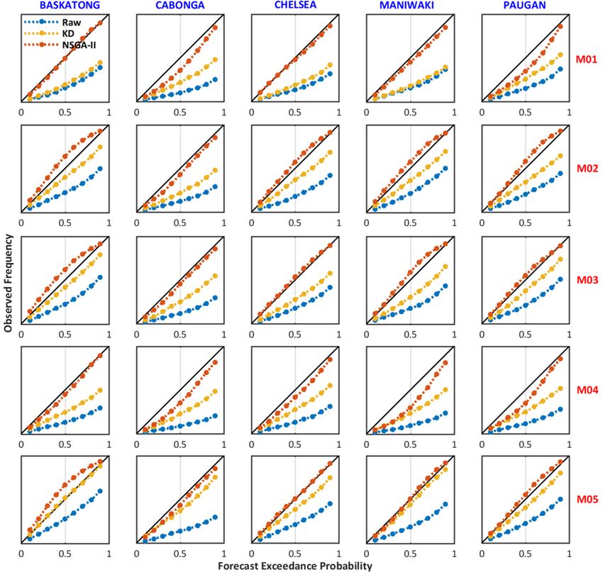
1002                                    J. Xu et al.: Exploring hydrologic post-processing of ensemble streamflow forecasts

and warning. Among them, the superiority of ensemble fore-          and the communication of integrated ensemble forecast prod-
casting systems in quantifying the propagation of predictive        ucts to end-users (e.g., operational hydrologists, water man-
uncertainties (over deterministic systems) is now well estab-       agers, local conservation authorities, stakeholders and other
lished (e.g., Cloke and Pappenberger, 2009; Palmer, 2002;           relevant decision-makers). Buizza et al. (2007) emphasized
Seo et al., 2006; Velázquez et al., 2009; Abaza et al., 2013;       that both functional and technical qualities are supposed to
Wetterhall et al., 2013; Madadgar et al., 2014). Numerous           be assessed for evaluating the overall forecast value of hy-
challenges have been well tackled; for example, (1) meteoro-        drological forecasts. Ramos et al. (2010) further note that
logical ensemble prediction systems (M-EPSs) (e.g., Palmer,         the best way to communicate probabilistic forecast and in-
1993; Houtekamer et al., 1996; Toth and Kalnay, 1997) are           terpret its usefulness should be in harmony with the goals of
refined and operated worldwide by the agencies such as              the forecasting system and the specific needs of end-users.
the European Centre for Medium-Range Weather Forecasts              Ramos et al. (2010) reported similar achievements from two
(ECMWF), the National Center for Environmental Predic-              studies obtained from a role play game and another survey
tion (NCEP), the Meteorological Service of Canada (MSC)             during a workshop (Thielen et al., 2005). During the work-
and more. (2) The forecast accuracy is highly improved by           shop, they explored the users’ risk perception of forecasting
adopting higher-resolution data collection and assimilation.        uncertainties and how they dealt with uncertain forecasts for
Sequential data assimilation techniques, such as the particle       decision-making. The results revealed that there is still space
filter (e.g., Moradkhani et al., 2012; Thirel et al., 2013) and     for enhancing the forecasters’ knowledge and experience on
the ensemble Kalman filter (EnKF; e.g., Evensen , 1994; Re-         bridging the communication gap between predictive uncer-
ichle et al., 2002; Moradkhani et al, 2005; McMillan et al.,        tainties quantification and effective decision-making.
2013) provide an ensemble of possible re-initializations of            Hence, in practice, which forecast quality impacts a given
the initial conditions, expressed in the hydrologic model as        decision the most? Different end-users share their unique
state variables such as soil moisture, groundwater level, and       requirements. Crochemore et al. (2017) produced the sea-
so on. (3) Forecasting skills of the coupled hydrometeorolog-       sonal streamflow forecasting by conditioning climatology
ical forecasting systems are also improved by tracking pre-         with precipitations indices (SPI3 – standardized precipitation
dictive errors using the full uncertainty analysis. Multimodel      index over 3 months). Forecast reliability, sharpness (i.e., the
schemes were proposed to increase performance and deci-             ensemble spread), overall performance, and low-flow event
pher the structural uncertainty (e.g., Duan et al., 2007; Fisher    detection were verified to assess the conditioning impact. In
et al., 2008; Weigel et al., 2008; Najafi et al., 2011; Velázquez   some cases, the reliability and sharpness could be improved
et al., 2011; Marty et al., 2015; Mockler et al., 2016). Thi-       simultaneously, while, more often, there was a trade-off be-
boult et al. (2016) compared many hydrologic ensemble pre-          tween them.
diction systems (H-EPSs), accounting for the three main                Here, two hydrological post-processors, namely the affine
sources of uncertainties located along the hydrometeorolog-         kernel dressing (AKD) and the evolutionary multi-objective
ical modeling chain. They pointed out that EnKF probabilis-         optimization (non-dominated sorting genetic algorithm II –
tic data assimilation provided most of the dispersion for the       NSGA-II), were explored. Compared to conventional post-
early forecasting horizons but failed in maintaining its effec-     processing methods, such as AKD, NSGA-II opens up the
tiveness with increasing lead times. A multimodel scheme            opportunity of improving the forecast quality in harmony
allowed for sharper and more reliable ensemble predictions          with the forecasting aims and the specific needs of end-users.
over a longer forecast horizon. (4) The statistical hydrologic      Multiple objective functions (i.e., here, verifying scores) for
post-processors, which have been added in the H-EPS for             evaluating the forecasting performances of the H-EPSs are
rectifying biases and dispersion errors (i.e., too narrow or        selected to guide the optimization process. The mechanisms
too large) are numerous, as reviewed by Li et al. (2017). It        of these two statistical post-processing methods are com-
is noteworthy that many hydrologic variables, such as dis-          pletely different. However, they share one similarity from an-
charge, follow a skewed distribution (i.e., low probability         other perspective, which is that they can estimate the proba-
associated to the highest streamflow values), which compli-         bility density directly from the data (i.e., ensemble forecast)
cates the task. Usually, in a hydrologic ensemble prediction        without assuming any particular underlying distribution. As a
system (H-EPS) framework (e.g., Schaake et al., 2007; Cloke         more conventional method, Silverman (1986) first proposed
and Pappenberger, 2009; Velázquez et al., 2009; Boucher et          the kernel density smoothing method to estimate the distri-
al., 2012; Abaza et al., 2017), the post-processing procedure       bution from the data by centering a kernel function K that
over the atmospheric input ensemble is often referred to as         determines the shape of a probability distribution (i.e., ker-
pre-processing. By correcting the bias and adjusting the dis-       nel) fitted around every data point (i.e., ensemble members).
persion based on a comparison with past observations, statis-       The smooth kernel estimate is then the sum of those kernels.
tical post-processing generally leads to a more accurate and        As for the choice of bandwidth h of each dressing kernel, Sil-
reliable hydrologic ensemble forecast.                              verman’s rule of thumb finds an optimal bandwidth h by as-
    However, another challenge still remains, namely how to         suming that the data are normally distributed. Improvements
improve the human interpretation of probabilistic forecasts         to the original idea were soon to follow. For instance, the

Hydrol. Earth Syst. Sci., 26, 1001–1017, 2022                                        https://doi.org/10.5194/hess-26-1001-2022
J. Xu et al.: Exploring hydrologic post-processing of ensemble streamflow forecasts                                           1003

improved Sheather–Jones (ISJ) algorithm is more suitable
and robust with respect to multimodality (Wand and Jones,
1994). Roulston and Smith (2003) rely on the series of best
forecasts (i.e., best member dressing) to compute the ker-
nel bandwidth h. Wang and Bishop (2005) and Fortin et al.
(2006) further improved the best member method. The lat-
ter advocated that the more extreme ensemble members are
more likely to be the best member of raw, under-dispersive
forecasts, while the central members tend to be more precise
for the over-dispersive ensemble. They proposed the idea that
different predictive weights should be set over each ensem-
ble member, given each member’s rank within the ensemble.
Instead of standard dressing kernels that act on individual
ensemble members, Bröcker and Smith (2008) proposed the
AKD method by assuming an affine mapping between en-
semble members and observation over the entire ensemble.
They approximate the distribution of the observation given
the ensemble.
   Given the single-model H-EPSs studied here, the hydro-
logic ensemble is generated by activating the following two       Figure 1. The five sub-catchments of the Gatineau River. The red
forecasting tools: the ensemble weather forecasts and the         thunder strike symbols locate the dams, while the original ECMWF
EnKF. Henceforth, enhancing the H-EPS forecasting skill by        grid points, before downscaling, are marked using black asterisks.
assigning different credibility to ensemble members becomes
preferred rather than reducing the number of members. The
post-processing techniques, like the non-dominated sorting        of both statistical post-processing methods in improving the
genetic algorithm II (NSGA-II), are now common (e.g., Li-         forecasting quality and enhancing the uncertainty communi-
ong et al., 2001; De Vos and Rientjes, 2007; Confesor and         cation are discussed and analyzed as well. The conclusion
Whittaker, 2007). Such techniques are conceptually linked to      follows in Sect. 5.
the multi-objective parameter calibration of hydrologic mod-
els using Pareto approaches. Indeed, formulating a model
structure or representing the hydrologic processes using a        2   The H-EPSs
unique global optimal parameter set proves to be very sub-
jective. Multiple optimal parameter sets exist with satisfy-      Figure 1 illustrates the study area, which is the Gatineau
ing behavior, given the different conceptualizations, although    River located in the southern Québec province, Canada. It
they are not identical Beven and Binley (1992). For example,      drains 23 838 km2 of the Outaouais and Montreal hydro-
Brochero et al. (2013) utilized the Pareto fronts generated       graphic region and experiences a humid continental climate.
with NSGA-II for selecting the best ensemble from a hydro-        The river starts from Sugar Loaf Lake (47◦ 52–54 N, 75◦ 30–
logic forecasting model with a pool of 800 streamflow pre-        43 W) and joins the Ottawa River some 400 km later. The av-
dictors in order to reduce the H-EPS complexity. Here, the        erage daily temperature is about −3 ◦ C in winter, while the
expected output of the NSGA-II method is a group of solu-         temperature spectrum is 10–22 ◦ C in summer (Kottek et al.,
tions, also known as Pareto front, that identify the trade-offs   2006). The hydrologic regime of the study area is generally
between different objectives, subject to the end-users’ needs     wet, cold, and snow covered. The largest flood typically ap-
and requirements.                                                 pears in spring or early summer (i.e., from March to June)
   In this study, the daily streamflow ensemble forecasts is-     from snowmelt and rainfall. Autumnal rainfall often leads to
sued from five single-model H-EPSs over the Gatineau River        a lesser peak between September and November (Fig. 2).
(province of Québec, Canada) are post-processed. Details              For operational hydrologic modeling, reservoir operation,
about the study area, hydrologic models, and hydrometeo-          and hydroelectricity production, the whole catchment has
rological data are described in Sect. 2. Section 3 explains       been divided up into the following five sub-catchments:
the methodology and training strategy of AKD and NSGA-II          Baskatong, Cabonga, Chelsea, Maniwaki, and Paugan (iden-
methods in parallel with the scoring rules that evaluate the      tified by different colors in Fig. 1). The sub-catchments are
performance of the forecasts. Specific concepts associated        modeled independently from one another in order to inform
with those scores are also introduced in this section. A pre-     a decision model operated by Hydro-Québec (e.g., Movahe-
dictive distribution estimation based on the five single-model    dinia, 2014). All hydroclimatic time series to the project were
H-EPS configurations, which lack accounting for the model         made available by Hydro-Québec, who carefully constructed
structure uncertainty, is presented in Sect. 4. The comparison    them for their own hydropower operations. Dams are identi-

https://doi.org/10.5194/hess-26-1001-2022                                      Hydrol. Earth Syst. Sci., 26, 1001–1017, 2022
1004                                      J. Xu et al.: Exploring hydrologic post-processing of ensemble streamflow forecasts

                                                                       Seiller et al., 2012). The empirical two-parameter model, Ce-
                                                                       maNeige (Valéry et al., 2014), simulates snow accumulation
                                                                       and melt. In this study, five representative models were se-
                                                                       lected from HOOPLA as typical examples. Their main char-
                                                                       acteristics are summarized in Table 2.
                                                                          The original observational time series extends from Jan-
                                                                       uary 1950 to December 2017, while, in terms of the in-
                                                                       put of HOOPLA, the observational period was limited to 33
                                                                       years (1985–2017) to avoid the increased bias and variability
                                                                       caused by missing values within the record. The meteoro-
                                                                       logical ensemble forecasts were retrieved from the European
                                                                       Center for Medium-Range Weather Forecasts (ECMWF;
                                                                       Fraley et al., 2010). The time series extends from Jan-
                                                                       uary 2011 to December 2016. The meteorological ensem-
                                                                       ble forecast used the reduced Gaussian transformation for the
                                                                       latitude–longitude system during the THORPEX Interactive
                                                                       Grand Global Ensemble (TIGGE) database retrieving by us-
                                                                       ing bilinear interpolation (e.g., Gaborit et al., 2013). The hor-
                                                                       izontal resolution was downscaled during the retrieval from
                                                                       the 0.5◦ ECMWF grid resolution to a 0.1◦ grid resolution.
                                                                       This study resorts to the 12:00 UTC (universal coordinated
Figure 2. Hydrograph of the daily streamflow (millimeters per day;     time) forecasts only, aggregated to a daily time step over a
hereafter mm d−1 ) averaged over each month during 33 years from       7 d horizon. All data are aggregated at the catchment scale,
1985 to 2017.                                                          averaging the grid points located within each sub-catchment.
                                                                       All of the time series were split in two, following the split-
Table 1. Hydroclimatic characteristics of five sub-catchments of the   sample test (SST) procedure of Klemeš (1986), with 1986–
Gatineau River.                                                        2006 for calibration and 2013–2017 for validation. In both
                                                                       cases, 3 prior years were used for the spin-up period. Jan-
   Name           Lat.     Long.     Catchment     Mean annual         uary 2011–December 2016 is committed to hydrologic fore-
                                     area (km2 )      Q (mm)           casting.
   Cabonga       47.21    −76.59          2665              1.35          Initial condition uncertainties within each H-EPS are
   Baskatong     47.21    −75.95         13 057             1.49       accounted for by a 100-member Ensemble Kalman Fil-
   Maniwaki      46.53    −76.25          4145              1.24       ter (EnKF) that adjusts the distribution function of the
   Paugan        46.07    −76.13          2790              1.29       model states given observational distributions. Meteorolog-
   Chelsea       45.70    −76.01          1142              1.27       ical uncertainties are quantified by providing the 50-member
                                                                       ECMWF ensemble forcing to the H-EPSs. The resulting en-
                                                                       semble streamflow forecasts thus consist of 5000 members.
fied in Fig. 1 as red thunder strike symbols. The two upper-           This setup is similar to the one described in more details by
most ones allow for the existence of large headwater reser-            Thiboult et al. (2016). The EnKF hyperparameters selection
voirs, while the other three are run-of-the-river installations.       follows the work of Thiboult and Anctil (2015). Streamflow
The daily streamflow (in cubic meters per second; hereafter            and precipitation uncertainties are assumed to be propor-
m3 s−1 ) time series entering the reservoirs were constructed          tional; they are set to 10 % and 50 %, respectively. Tempera-
by the electricity producer from a host of local information           ture uncertainty is considered constant; it amounts to 2 ◦ C. A
and made available to the study, along with spatially aver-            Gaussian distribution describes the streamflow and tempera-
aged minimum and maximum air temperature (degrees Cel-                 ture uncertainty, and a gamma law represents the precipita-
sius) and precipitation (millimeters) for each sub-basin. Ta-          tion uncertainty.
ble 1 summarizes the various hydroclimatic characteristics
of the Gatineau River sub-catchments. Potential evapotran-
spiration is calculated from the temperature-based Oudin et            3   Methodology
al. (2005) formulation.
   The HydrOlOgical Prediction LAboratory (HOOPLA;                     This study was conducted on the base of 1–7 d ensemble
Thiboult et al., 2020, https://github.com/AntoineThiboult/             streamflow forecasts issued from five single-model H-EPSs
HOOPLA) provides a modular framework to perform cali-                  and their realizations. Both AKD and NSGA-II methods are
bration, simulation, and streamflow prediction using multiple          utilized in this study as the statistical post-processing or so-
hydrologic models (up to 20 lumped models; Perrin, 2002;               called ensemble interpretation method (Jewson, 2003; Gneit-

Hydrol. Earth Syst. Sci., 26, 1001–1017, 2022                                           https://doi.org/10.5194/hess-26-1001-2022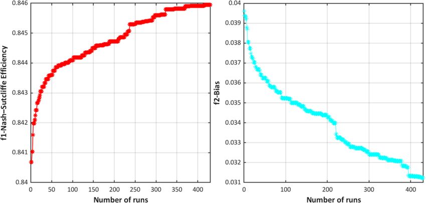
J. Xu et al.: Exploring hydrologic post-processing of ensemble streamflow forecasts                                                     1005

Table 2. Main characteristics of the hydrologic models (Seiller et al., 2012).

                          Model      No. of optimized       No. of     Model derived from
                                           parameters    reservoirs
                          M01                        6            3    BUCKET (Thornthwaite and Mather, 1955)
                          M02                        4            2    GR4J (Perrin et al., 2003)
                          M03                        9            3    HBV (Bergström et al., 1973)
                          M04                        7            3    IHACRES (Jakeman et al., 1990)
                          M05                        9            5    SACRAMENTO (Burnash et al., 1973)

ing et al., 2005) to transform the raw ensemble forecast into             venience, as follows:
a probability distribution.
                                                                                            2
                                                                                   1     1
3.1   Affine kernel dressing (AKD)                                        K (·) = √ exp − (·) .                                           (4)
                                                                                   2π    2
Rather than adopting the ensemble mean and the standard                     The mean and the variance of the interpreted ensemble can
deviation and approximate the distribution of the raw en-                 be defined as follows:
semble (Wilks, 2002), the principal insight of this method-
ology is that the probability distribution could be fitted of the                             1X
                                                                          µ0 (X) = b + a ·         xi = b + a · µ (X)                     (5)
observation when given the ensemble (Bröcker and Smith,                                      m i
2008). The AKD method interprets the ensemble by ap-
                                                                                               1X
proximating the distribution of the observation when given                υ 0 (X) = h2 + a 2 ·      [xi − µ (X)]2 = h2 + a 2 · υ (X).     (6)
the ensemble forecasts. The ordering of the ensemble mem-                                      m i
bers is not taken into account (i.e., ensemble members are
considered exchangeable here). Here, we denote the en-                       The mapping parameters of a, b, and h are determined
semble forecasts with m members over time t by X(t) =                     from the raw ensemble. The updated mean µ0 (X) of the
[x1 (t), x2 (t), . . ., xm (t)] and the observation by y(t). The          kernel-dressed ensemble is a function of the raw ensemble
mean and the variance of the raw ensemble forecasts are then              mean µ (X), which is scaled and shifted using a and b. The
as follows:                                                               variance υ 0 (X) of the kernel-dressed ensemble is a function
                                                                          of the initial ensemble variance υ (X), which is scaled and
        1X                                                                shifted using a 2 and h2 . Detailed derivations of these equa-
µ (X) =     xi                                                   (1)
        m i                                                               tions are given by Bröcker and Smith (2008).
                                                                             AKD provides the solutions for determining the parame-
        1X
υ (X) =     [xi − µ (X)]2 .                                      (2)      ters of a, b, and h, which are determined as functions of X,
        m i                                                               as follows:
   In a general form, the probability density function of
p (y; X, θ ) defines the interpreted ensemble (i.e., kernel-
                                                                          b = r1 + r2 · µ (X)                                             (7)
dressed ensemble), given the original ensemble with free pa-                        h                     i
rameter vector θ , as follows:                                            h2 = h2S · s1 + s1 · a 2 · υ (X)                                (8)
                                                                                              1/5
                                                                        hS = 0.5 · 4/ (3m)         .                                    (9)
                1 X     y − axi − b
p (y; X, θ ) =      K                 ,                          (3)
               bh i          h                                               Here, hS is Silverman’s factor (Silverman, 1986). Techni-
                                                                          cally, we can use some scores (e.g., mean square error) to se-
for which the interpreted ensemble can be seen as a sum                   lect the optimal bandwidth h for a kernel density estimation,
of probability functions (kernels) around each raw ensem-                 yet this would be difficult to estimate for general kernels.
ble member. xi represents the ith ensemble member, and y is               Hence, the first rule of thumb proposed by Silverman gives
the corresponding observation. Hence, axi + b identifies the              the optimal bandwidth h which is the standard deviation of
center of each kernel using the scale parameter a and offset              the distribution. And in this case, the kernel is also assumed
parameter b. h is the positive bandwidth of each kernel. Note             to be Gaussian. The parameters θ = [a, r1 , r2 , s1 , s2 ] are free
that various distributions could be adopted as kernels (Silver-           parameters, and usually r1 = 0, r2 = 1, s1 = 0 and r2 = 1 are
man, 1986; Roulston and Smith, 2003; Bröcker and Smith,                   rational initial selections (Bröcker and Smith, 2008). Once
2008). We opted for the standard Gaussian density function                the optimal free parameter vector θ = [a, r1 , r2 , s1 , s2 ] is ob-
with zero mean and unit variance for its computational con-               tained, the interpreted ensemble can be set to the following:

https://doi.org/10.5194/hess-26-1001-2022                                               Hydrol. Earth Syst. Sci., 26, 1001–1017, 2022
1006 J. Xu et al.: Exploring hydrologic post-processing of ensemble streamflow forecasts
needed when we verify whether an H-EPS is competent at
issuing accurate and reliable forecasts. Accuracy might be
1 X y − axi − b the first idea that crosses our mind and indicates that there
p (y; X, θ ) = K
bh i h is a good match between the forecasts and the observations.
1 X
y − zi
Since here we are focused on probabilistic streamflow fore-
= K (10) cast, the accuracy could be measured by computing the dis-
bh i h
tances between the forecast densities with the observations
zi = axi + r2 · µ (X) + r1 (11) (Wilks, 2011). Usually, hydrologists could rely on the Nash–
h2 = h2S · [s1 + s2 · υ (X)] , (12) Sutcliffe efficiency criterion (NSE; Nash and Sutcliffe, 1970)
for measuring how well forecasts can reproduce the observed
where Zi is the resulting kernel-dressed ensemble based on time series. Transforming the time series beforehand allows
the raw ensemble X and fitted parameters a, r1 , and r2 . one to specialize it (i.e., NSEinv , NSEsqrt ) for specific needs
Bröcker and Smith (2008) stressed that this AKD ensemble (e.g., Seiller et al., 2017). NSE is dimensionless and varies
transformation works on the whole ensemble rather than on on the interval of [−∞, 1]. NSE is attained by dividing the
each individual member. Finally, the mean and variance of mean square error (MSE) by the variance of the observations
the interpreted ensemble shown in Eqs. (5) and (6) can be and then subtracting that ratio from 1.
rewritten as follows: PT
MSE (xt − yt )2
NES = 1 − = 1 − Pt=1
T 2
, (15)
var(y) t=1 (yt − y)
µ0 (X) = b + a · µ (X) = r1 + (a + r2 ) · µ (X) (13)
where xt and yt are the forecasted and observed values at
υ 0 (X) = h2 + a 2 · υ (X) = h2S · s1 + a 2 · h2S · s2 + 1 time step t, respectively. y and var(y) represent the mean and
· υ (X) . (14) variance of the observations. A perfect model forecast output
would have an NSE value that equals to one.
3.2 Non-dominated sorting genetic algorithm II Meanwhile, bias, also known as systematic error, refers
(NSGA-II) to the correspondence between the average forecast and the
average observation, which is different from accuracy. For
Multi-objective optimization problems are common and typ- example, systematic bias exists in the streamflow forecasts
ically lead to a set of optimal options (Pareto solution set) that are consistently too high or too low. Hence, NSE and bias
for users to choose from. Exploiting a genetic algorithm to are utilized here as objective functions, which is to say that
find out all Pareto solutions from the entire solution space they are seeking to minimize the bias and maximize the NSE
have been proposed and improved since the publication of simultaneously. This brings us a multi-objective optimization
the vector evaluated genetic algorithm (VEGA) around 1985 question to solve.
(Schaffer, 1985). Technically, inserting the elitism in the multi-objective op-
There exist two main standpoints for dealing with multi- timization algorithms is not compulsory. However, it would
objective optimization problems, namely to (1) define a new have a strong influence if the algorithms could preserve the
objective function as the weighted sum of all desired ob- best individuals (i.e., elites) that were found during the search
jective functions (e.g., MBGA, migrating-based genetic al- process and then incorporate the elitism back into the evolu-
gorithm, and RWGA, random weighted genetic algorithm) tionary process (Groşaelin et al., 2003). A classic, fast, and
or to (2) determine the Pareto set or its representative sub- elitist multi-objective genetic algorithm, the non-dominated
sets for a selected group of objective functions (e.g., SPEA sorting genetic algorithm II (NSGA-II; Deb et al., 2002) is
(strength Pareto evolutionary Algorithm), SPEA-II, NSGA, adopted for searching for the Pareto solution set. NSGA-II
and NSGA-II). The first approach is more trivial as it re- offers three specific advantages over previous genetic algo-
duces to a single-objective optimization problem. Yet, the rithms. (1) There is no need to specify extra parameters such
needed weighting strategy is difficult to set accurately as a as the niche count for the fitness sharing procedure, (2) it re-
minor difference in weights may lead to quite different so- duces complexity over alternative GA implementations, and
lutions. On the other hand, Pareto ranking approaches have (3) elite individuals are well maintained, and hence, the ef-
been devised in order to avoid the problem of converging to- fectiveness of the multi-objective genetic algorithm is largely
wards solutions that only behave well for one specific ob- improved.
jective function. Users still have to select objective functions In this study, the population is denoted by X(t). Specific
that are pertinent to the problem and that are not heavily cor- steps for NSGA-II are briefly introduced here.
related to one another. Readers may refer to the review by
Konak et al. (2006) for more details. 1. Layer the whole population by using the fast non-
Similar ideas can be utilized in this study, as the goal is dominated sorting approach. i is initially set to 1, while
to achieve a good forecast. Various efficiency criteria are zi represents the ith solution among the m ones. We
Hydrol. Earth Syst. Sci., 26, 1001–1017, 2022 https://doi.org/10.5194/hess-26-1001-2022J. Xu et al.: Exploring hydrologic post-processing of ensemble streamflow forecasts 1007
compare the domination and non-domination relation- 3.3 Verifying metrics
ship between the individuals zi and zj for all the j =
1, 2, . . ., m, and i 6 = j . zi is the non-dominated solution The performance of the post-processed forecast distributions,
as long as no zj dominates it. This process is repeated mostly in terms of accuracy and reliability, is assessed us-
until all the non-dominated solutions are found and have ing scoring rules. Except for bias and NSE described above,
composed the first non-dominated front of the popula- seven other verifying scores are applied to both the raw and
tion. Note that the selected individuals of the first front post-processed forecast distributions.
can be neglected when searching for subsequent fronts The overall accuracy and reliability of the probabilistic
(i.e., marked as krank ). forecast can be evaluated using the continuous ranked prob-
ability score (CRPS; Matheson and Winkler, 1976; Hers-
2. Find the crowding distance for each individual in each bach, 2000; Gneiting and Raftery, 2007). Hersbach (2000)
front. Deb et al. (2002) pointed out that the basic idea of decomposed the CRPS into two parts, i.e., reliability and res-
the crowding distance calculated in the NSGA-II is “to olution. In practice, The mean continuous ranked probabil-
find the Euclidian distance between each individual in a ity score (MCRPS) is the average value of CRPS over the
front based on their m objectives in the m-dimensional whole time series T and is calculated using empirical dis-
hyper space. The individuals in the boundary are always tributions. Besides, MCRPS is negatively oriented, and the
selected since they have infinite distance assignment. optimal MCRPS value is 0, as follows:
The large average crowding distance will result in better
diversity in the population”. This step ensures the diver- +∞
T Z
1X 2
sity of the population. For example, for the first front, MCRPS = Ptfcst (y) − H yt ≥ ytobs dy, (17)
sort the values of the objective functions in an ascend- T t=1
−∞
ing order. The boundary solutions (i.e., maximum and
minimum solutions) are then the value at infinity. The where y is the predictand, and ytobs represents the corre-
crowding distance for other individuals can be assigned sponding observations. Ptfcst (y) is the cumulative distribu-
as follows: tion function of the forecasts at time step t. The Heaviside
function H equals 0 (or 1) when yt < ytobs (or yt ≥ ytobs ).
As for the deterministic metrics, we adopt the mean abso-
m
X Zj +1 Zj −1 lute error (MAE) and root mean squared error (RMSE; e.g.,
kdistance = − , (16) Brochero et al., 2013) to verify the average forecast error of
k=1 n n the variable of interest. Both MAE and RMSE are negatively
oriented and range from 0 to +∞. More accurate forecasts
where kdistance represents the value for the kth individ- lead to lower MAE and RMSE. Note that the RMSE score
j +1 j −1
ual, and fn and fn are the values of the nth objec- tends to penalize the large errors more than MAE. In some
tive function at j + 1 and j − 1, separately. Thereafter, cases, where the variance corresponding to the frequency dis-
the crowding comparison operator can be utilized based tribution is higher, the RMSE will have larger increase while
on krank and kdistance . Individual zi will be assumed su- the MAE remains stable.
i j i j
perior to zj if krank < krank , or kdistance > kdistance , when RMSE has the benefit of penalizing large errors more, so
their Pareto front ranks are equal. it can be more appropriate in some cases.
The Kling–Gupta efficiency (KGE; Gupta et al., 2009)
3. Elitism strategy is introduced in the main loop. Off-
also allows for a comprehensive performance assessment of
spring population Qt is firstly generated from the parent
the deterministic forecasts. KGE’, a slightly modified version
population Pt after mutation and gene crossover. Then
of KGE (Kling et al., 2012), avoids any cross-correlation be-
the abovementioned non-dominated sorting and crowd-
tween the bias and the variability ratios. It is defined as fol-
ing distance assignment are conducted on the composed
lows:
population Rt that contain both Qt and Pt with the size
q
of 2 m. The first-rate non-dominated solutions will be
KGE0 = (r − 1)2 + (β − 1)2 + (γ − 1)2 (18)
assign to the new parent population Pt+1 . Outputs after
the whole evolutionary search are the un-repeated non- µy
β= (19)
domination solutions, and a weight matrix can also be µo
extracted from the solutions. Specifically, in this study, CVy σy / uy
γ= = . (20)
the population size is set to 50, the number of objective CVo σo / uo
functions equals to 2, the boundary is from 0 to 1, the
mutation probability and crossover rate are 0.1 and 0.7, The correlation coefficient r represents the linear associa-
respectively, and the maximum evolution runs are 430 tion between the deterministic forecast and the observations.
times. µy (µo ) and σy (σo ) are the mean and the standard deviations
of the forecasts (here it is the ensemble mean) and obser-
https://doi.org/10.5194/hess-26-1001-2022 Hydrol. Earth Syst. Sci., 26, 1001–1017, 20221008 J. Xu et al.: Exploring hydrologic post-processing of ensemble streamflow forecasts
vation, respectively. CV is the dimensionless coefficient of tain the kernel-dressed ensemble. Note that AKD acts
variation. on the entire ensemble rather than on each individual
The reliability diagram (Stanski et al., 1989) is a graphi- member.
cal representation of the reliability of an ensemble forecast.
It contrasts the observed frequency against the probability of 3. Evaluate the Pareto fronts (i.e., non-dominated solu-
ensemble forecasts over all quantiles of interest. The prox- tions that minimize/maximize the bias and the NSE) and
imity from the diagonal line indicates how closely the fore- the weight matrix by applying NSGA-II over the train-
cast probabilities are associated to the observed frequencies ing dataset. Sloughter et al. (2007) mentioned that the
for selected quantiles. The 45◦ diagonal line thus represents training period should be specific for each dataset or re-
perfect reliability, i.e., when the ensemble forecast probabili- gion. Here, a 30 d moving window is selected so that it
ties equals the observation ones. When the plotted curve lies contains enough training samples with coherent consis-
above the 45◦ line, the predictive ensemble is over-dispersed. tency, which is to say that the NSGA-II post-processors
It is otherwise under-dispersed. In addition, a flat curve rep- were trained using only the past 30 d and day 4 fore-
resents that the forecast has no resolution (i.e., climatology). cast data and then re-trained for every following day.
The spread skill plot (SSP or later simply referred to as From the operational perspective, a monthly moving
spread; Fortin et al., 2014) assesses the ensemble spread and window is especially more coherent and efficient in the
identifies an ensemble forecast with poor predictive skill and real world, with a limited length for the time series.
large dispersion that would be positively assessed by a relia-
bility diagram. Fortin et al. (2014) stresses that the ensemble A general flowchart of the streamflow input, AKD and
spread should match the RMSE of the ensemble mean when NSGA-II frameworks, and expected outputs is illustrated in
the predictive ensemble is reliable. Thus, the SSP comple- Fig. 3.
ments the spread component with an accuracy aspect.
4 Results and discussions
3.4 Experimental setup
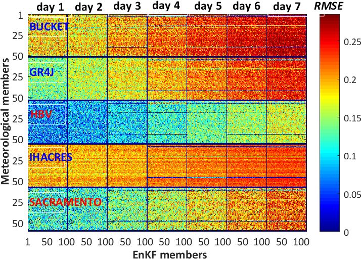
4.1 Ensemble member exchangeability
Establishing and analyzing both AKD and NSGA-II predic-
tive models to interpret single-model hydrologic ensemble The issue of member interchangeability is central to this
forecasts for uncertainty analysis can be summarized in three study, since, for AKD, each raw ensemble will be consid-
steps. ered as a whole (i.e., indistinguishable members), whereas
1. Determine the training period. Subject to the dataset for NSGA-II a weight matrix is sought, which implies that
used in this study, it can be considered to have two different weights are assigned to each candidate members.
components, namely the observations/forecasts that last Interchangeability is here assessed visually, by simulta-
from January 2011 to December 2016 and the target neously looking at the individual RMSE values of all 5000
ensemble for interpretation with a forecasting horizon members, seven daily forecast horizons, and five H-EPSs.
that extends from day 1 to 7. Here, a common calibra- Figure 4 displays the (typical) values for day 500 and Baska-
tion/validation procedure was conducted on the second tong sub-catchment. The animation screenshots covering the
component of the dataset. We conducted the calibration different stages along the full time series are available in the
on the day 4 forecast and then tested it on other lead Supplement. For each H-EPS forecast horizon box, horizon-
times to assess the robustness of the predictive mod- tal lines consist of 100 EnKF members and vertical lines with
els. The skill of hydrologic forecasts fades away with 50 meteorological members. Mosaics with redder colors rep-
increasing lead time. The 4 d ahead ensemble forecasts resent higher values of the RMSE. The decreasing predictive
issued from each single-model H-EPSs and their corre- skill of the H-EPSs with lead time is, hence, shown as an
sponding observations are chosen as a training dataset, increasingly red mosaic.
since they are located in the middle of the forecast hori- Figure 4 displays the hydrologic forecasts built upon the
zon. The validation dataset then consists of the remain- 50-member ECMWF ensemble forecasts. The basic idea be-
ing forecasts, i.e., 1–3 and 5–7 d ahead raw forecasts hind Fig. 4 (and its accompanying video) is to visually assess
issued from the associated H-EPSs. The procedure was if the initial interchangeability of the weather forecasts holds
selected as a specific example. Yet, one may decide oth- for the hydrologic forecasts (i.e., horizontal lines), while
erwise, such as implementing the calibration/validation the interchangeability of the probabilistic data assimilation
procedures separately for each day. scheme is assessed in parallel (vertical lines). One can no-
tice that, in Fig. 4, colorful horizontal lines within each box
2. AKD mapping between the ensemble and observation start to appear from day 3 onwards, revealing a distinguish-
over the training dataset. The observation time se- able character with longer lead times. At the same time, no
ries are used to identify the free parameter vector θ = obvious vertical lines are present in the same figure. These
[a, r1 , r2 , s1 , s2 ], thereby minimizing the MCRPS to ob- results suggest that the hydrologic forecasts produced in this
Hydrol. Earth Syst. Sci., 26, 1001–1017, 2022 https://doi.org/10.5194/hess-26-1001-2022J. Xu et al.: Exploring hydrologic post-processing of ensemble streamflow forecasts 1009
Figure 3. Schematic of the experimental setup flowchart.
Figure 4. Illustration of the RMSE values (mm d−1 ) of the indi-
vidual members of the forecast issued by the five H-EPSs for the
Baskatong sub-catchment on day 500. There are seven daily fore-
cast horizons. Each box consists of 5000 members, including 100 Figure 5. NSGA-II Pareto fronts of the model M01 over the Baska-
EnKF members (horizontal lines) and 50 meteorological members tong catchment. Horizontal and vertical axis are NSE and bias, sep-
(vertical lines). arately.
study are fully interchangeable with respect to EnKF but less multi-objective evolutionary search, 35 (non-dominated)
so with respect to the weather, with the latter being nonlin- Pareto solutions are identified. No objective can be im-
early transformed by the hydrologic models. This opens up proved more without the sacrifice of another. The optimal
the possibility of assigning weights to the hydrologic fore- NSE is inevitably accompanied with the highest bias (e.g.,
casts associated to the ECMWF members. NSE = 0.84594; bias = 0.034055) or vice versa. The solu-
For practical reasons, as the 100-member data assimilation tions in the elbow region of the Pareto front are the com-
ensemble was deemed to be fully interchangeable, this com- promise between both two objective functions. Pareto fronts
ponent is randomly reduced to 50 members from now on in with different numbers of solutions can be attained daily via
this document. This procedure simplifies the implementation setting the sliding window. Therefore, rather than choosing
of the AKD and NSGA-II post-processing computations, the only one fixed position in the front, we opted to pick the so-
results of which are presented next. lution randomly to respect and explore the diversity within.
Figure 6 confirms the NSGA-II convergence.
4.2 NSGA-II convergence
The NSGA-II Pareto front drawn in Fig. 5 (model M01
over the Baskatong catchment) is quite typical. In this
https://doi.org/10.5194/hess-26-1001-2022 Hydrol. Earth Syst. Sci., 26, 1001–1017, 20221010 J. Xu et al.: Exploring hydrologic post-processing of ensemble streamflow forecasts Figure 6. NSGA-II dynamical performance plots for both objective functions vs. the number of evaluations for model M01 over Baskatong catchment. Figure 7. Forecasting reliability of the raw, AKD, and NSGA-II forecasts on the calibration dataset (4 d ahead forecast) for five single-model H-EPSs over each individual catchment (January 2011–December 2016). Hydrol. Earth Syst. Sci., 26, 1001–1017, 2022 https://doi.org/10.5194/hess-26-1001-2022
J. Xu et al.: Exploring hydrologic post-processing of ensemble streamflow forecasts                                         1011

Figure 8. Accuracy performance assessment of the raw, AKD, and NSGA-II forecasts (4 d ahead forecast) for five single-model H-EPSs
over each sub-catchment of the Gatineau catchment (January 2011–December 2016).

https://doi.org/10.5194/hess-26-1001-2022                                       Hydrol. Earth Syst. Sci., 26, 1001–1017, 2022
1012 J. Xu et al.: Exploring hydrologic post-processing of ensemble streamflow forecasts
4.3 AKD and NSGA-II performance comparison 5 Conclusions
The reliability of the raw, kernel-dressed, and NSGA-II pre- Hydrologic post-processing of streamflow forecasts plays an
dictive distributions with different lead times are displayed in important role in correcting the overall representation of un-
the reliability diagrams of Fig. 7. Both post-processing meth- certainties in the final streamflow forecasts. Both the ker-
ods improve over the raw ensemble, especially the NSGA- nel ensemble dressing and the evolutionary multi-objective
II, as it achieves the best reliability. Over-dispersion exists optimization approaches are tested in this study to estimate
mainly over the Baskatong catchments for NSGA-II. the probability density directly from the data (i.e., daily
The relevant accuracy performances of the raw, AKD, and ensemble streamflow forecast) over five single-model hy-
NSGA-II predictive models are summarized using radar plots drologic ensemble prediction systems (H-EPSs). The AKD
in Fig. 8. We can notice that the kernel-dressed ensemble fails method provides an affine mapping between the entire en-
in decreasing the forecast bias. However, it adjusts the en- semble forecast and the observations without any assumption
semble dispersion properly. As for the NSGA-II, the post- of the underlying distributions. The Pareto fronts generated
processed ensemble has an obvious improvement on both with NSGA-II relax the parametric assumptions regarding
bias and ensemble dispersion. Accordingly, it demonstrates the shape of the predictive distributions and offer trade-offs
a very reliable performance, as shown in the reliability dia- between different objectives in a multi-score framework.
gram. The single-model H-EPSs explored in this study account
The trained optimal free parameter vector θ = for both forcing uncertainty and initial conditions uncer-
[α, r1 , r2 , s1 , s2 ] or weight estimates are obtained over tainty by using ensemble weather forecasts (ECMWF) and
the 4 d ahead ensemble forecasts. They are then applied to data assimilation (EnKF). Hydrologic post-processing with
the validation dataset. It comprises the 1, 3, 5, and 7 d ahead AKD and NSGA-II rely on very different assumptions and
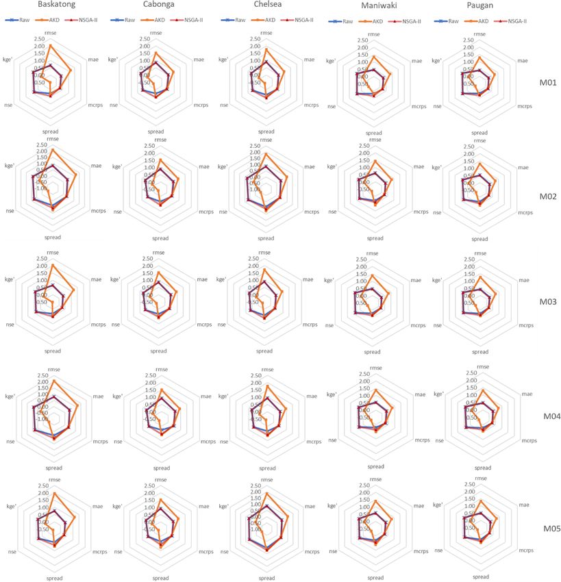
raw forecasts issued from the associated H-EPSs. Figure 9 methodology. However, they both transform the raw ensem-
shows the reliability diagrams for raw, kernel-dressed, bles into probability distributions. Results show that the post-
and NSGA-II forecasts for the validation dataset over five processed forecasts achieve stronger predictive skill and bet-
individual catchments. Therefore, there are 15 lines shown ter reliability than raw forecasts. In particular, the NSGA-
in each sub-diagram. Again, raw forecasts (i.e., blue lines) II post-processed forecasts achieve the most reliable perfor-
display a severe under-dispersion, revealing that error growth mances, since this method improves both bias and ensem-
is not maintained well in a single-model H-EPS. In general, ble dispersion. However, over-dispersion may exist occasion-
the other two statistical post-processing methods succeed ally over the Baskatong catchment for NSGA-II. The kernel-
in improving the forecast reliability, with the curves closer dressed ensemble succeeds in adjusting the ensemble disper-
to the bisector lines. The NSGA-II (i.e., red curves) espe- sion properly but bias increases. Note that, here, we cali-
cially demonstrates its superior ability for maintaining the brated the models on day 4 and then tested them on the other
reliability with the lead time. The over-dispersion appears days to assess the robustness of the procedure. The results
with most of the AKD transformed ensembles (i.e., yellow show that both AKD and NSGA-II predictive models could
lines), especially at shorter lead times. The ensemble spread offer an efficient post-processing skill, and the procedure is
tends to a proper level as the lead time increases. Note that quite robust as well. Others may try alternatives such as im-
there is one special case where the predictive distributions of plementing the models separately on other lead times.
the kernel-dressed ensemble are the most reliable for model In the operational field, not only quantifying but also com-
M05 over almost all individual catchments. municating the predictive uncertainties in probabilistic fore-
Figure 10 demonstrates the ensemble spread with different casts will become an essential topic. As mentioned in the
forecasting horizons on the x axis and shows the changing introduction, another challenge that remains is how we can
performance trend. Clearly, both the kernel-dressed ensem- bridge the communication gap between the forecasters’ and
ble and NSGA-II predictive forecasts have increased disper- the end-users’, such as the operational hydrologists, local
sion for all models over all catchments and result in more conservation authorities, and some other relevant stakehold-
reliable predictive distributions. Figure 10 also provides an ers, interpretation about probabilistic forecasts. What fac-
intuitive reference of the accuracy performance of the raw, tor may have the strongest impact on decision-making? The
AKD, and NSGA-II interpreted ensemble forecasts in terms different end-users may have their unique preferences and
of the MAE, MCRPS, and the ensemble dispersion for differ- demands. For instance, the reliability and sharpness (i.e.,
ent forecasting horizons, showing the evolution of forecast- spread) could be improved simultaneously, or there could be
ing performance. Clearly, both the kernel-dressed ensemble a trade-off between them.
and NSGA-II forecasts have increased dispersion compared In this paper, the performance of the NSGA-II method is
to raw forecasts for all models and over all catchments. This compared with a conventional post-processing method, i.e.,
results in more reliable predictive distributions, as shown in the AKD. NSGA-II demonstrated its superior ability in im-
Fig. 9. proving the forecast performance and communicating trade-
offs with end-users on which performance aspects to improve
Hydrol. Earth Syst. Sci., 26, 1001–1017, 2022 https://doi.org/10.5194/hess-26-1001-2022J. Xu et al.: Exploring hydrologic post-processing of ensemble streamflow forecasts 1013 Figure 9. Comparison of the reliability of the raw, kernel-dressed, and NSGA-II forecasts on the validation dataset (i.e., 1–3 and 5–7 d ahead forecasts) for five singe-model H-EPSs over all catchments (January 2011–December 2016). Figure 10. Comparison of the MAE, MCRPS, and ensemble dispersion of the raw, AKD, and NSGA-II forecasts (i.e., 1–3 and 5–7 d ahead forecasts) for five singe-model H-EPSs over all catchments (January 2011–December 2016). The x axis for each sub-plot represents different horizons. https://doi.org/10.5194/hess-26-1001-2022 Hydrol. Earth Syst. Sci., 26, 1001–1017, 2022
1014                                       J. Xu et al.: Exploring hydrologic post-processing of ensemble streamflow forecasts

most. As the selected objective functions here, neither NSE              Financial support. This research has been supported by the Natu-
nor bias could be improved more without negatively impact-               ral Sciences and Engineering Research Council of Canada (grant
ing the other. The use of NSGA-II opens up opportunities to              nos. NETGP 451456-13 and RGPIN-2020-04286).
enhance the forecast quality in line with the specific needs
of the end-users, since it allows for setting multiple specific
objective functions from scratch. This flexibility should be             Review statement. This paper was edited by Dimitri Solomatine
considered as a key element for facilitating the implementa-             and reviewed by three anonymous referees.
tion of H-EPSs in real-time operational forecasting.

                                                                         References
Code availability. Tools used in this study are open
to the public. The scripts related to this article are                   Abaza, M., Anctil, F., Fortin, V., and Turcotte, R.: A comparison
available      on    GitHub     (https://github.com/BaoMTL/hess;           of the Canadian global and regional meteorological ensemble
https://doi.org/10.5281/zenodo.6113443, Jing, 2022).                       prediction systems for short-term hydrological forecasting, Mon.
                                                                           Weather Rev., 141, 3462–3476, https://doi.org/10.1175/MWR-
                                                                           D-12-00206.1, 2013.
Data availability. All the datasets used in this study are open to the   Abaza, M., Anctil, F., Fortin, V., and Perreault, L.: Hy-
public. The ensemble prediction system studied in this research was        drological Evaluation of the Canadian Meteorological En-
built from the HydrOlOgical Prediction LAboratory (HOOPLA),                semble Reforecast Product, Atmos. Ocean., 55, 195–211,
which is available on GitHub (https://github.com/AntoineThiboult/          https://doi.org/10.1080/07055900.2017.1341384, 2017.
HOOPLA, Thiboult et al., 2019). ECMWF meteorological en-                 Ajami, N. K., Duan, Q., and Sorooshian, S.: An integrated hy-
semble forecast data can be retrieved freely from the TIGGE                drologic Bayesian multimodel combination framework: Con-
data portal (https://apps.ecmwf.int/datasets/data/tigge/levtype=sfc/       fronting input, parameter, and model structural uncertainty
type=cf/, Bougeault et al., 2010). The observed datasets were pro-         in hydrologic prediction, Water. Resour. Res., 43, 1–19,
vided by the Direction d’Expertise Hydrique du Québec and can be           https://doi.org/10.1029/2005WR004745, 2007.
obtained on request for research purposes.                               Bergström, S. and Forsman, A.: Development of a conceptual de-
                                                                           terministic rainfall-runoff model, Nord. Hydrol., 4, 147–170,
                                                                           https://doi.org/10.2166/nh.1973.0012, 1973.
Supplement. The supplement related to this article is available on-      Beven, K. and Binley, A.: GLUE: 20 years on, Hydrol. Process., 28,
line at: https://doi.org/10.5194/hess-26-1001-2022-supplement.             5897–5918, https://doi.org/10.1002/hyp.10082, 2014.
                                                                         Beven, K. and Binley, A.: The future of distributed models: Model
                                                                           calibration and uncertainty prediction, Hydrol. Process., 6, 279–
                                                                           298, https://doi.org/10.1002/hyp.3360060305, 1992.
Author contributions. JX, FA, and MAB designed the theoretical
                                                                         Bougeault, P., Toth, Z., Bishop, C., Brown, B., Burridge, D., Chen,
formalism. JX performed the analytic calculations. Both FA and
                                                                           D. H., Ebert, B., Fuentes, M., Hamill, T. M., Mylne, K., Nico-
MAB supervised the project and contributed to the final version of
                                                                           lau, J., Paccagnella, T., Park, Y.-Y., Parsons, D., Raoult, B.,
the paper.
                                                                           Schuster, D., Silva Dias, P., Swinbank, R., Takeuchi, Y., Ten-
                                                                           nant, W., Wilson, L., and Worley, S.: The THORPEX interactive
                                                                           grand global ensemble, B. Am. Meteorol. Soc., 91, 1059–1072,
Competing interests. The contact author has declared that neither          https://doi.org/10.1175/2010BAMS2853.1, 2010 (data available
they nor their co-authors have any competing interests.                    at: https://apps.ecmwf.int/datasets/data/tigge/levtype=sfc/type=
                                                                           cf/, last access: 6 February 2022).
                                                                         Buizza, R., Asensio, H., Balint, G., Bartholmes, J., Bliefernicht, J.,
Disclaimer. Publisher’s note: Copernicus Publications remains              Bogner, K., Chavaux, F., de Roo, A., Donnadille, J., Ducrocq,
neutral with regard to jurisdictional claims in published maps and         V., Edlund, C., Kotroni, V., Krahe, P., Kunz, M., Lacire, K.,
institutional affiliations.                                                Lelay, M., Marsigli, C., Milelli, M., Montani, A., Pappen-
                                                                           berger, F., Rabufetti, D., Ramos, M. -H., Ritter, B., Schipper,
                                                                           J, W., Steiner, P., J. Del Pozzo, T., and Vincendon, B.: EU-
Acknowledgements. Funding for this work was provided by Flood-             RORISK/PREVIEW report on the technical quality, functional
Net, an NSERC Canadian Strategic Network, and by an NSERC                  quality and forecast value of meteorological and hydrological
Discovery Grant. We would like to thank Emixi Sthefany Valdez,             forecasts, ECMWF Technical Memorandum, ECMWF Research
who provided the ensemble forecast data that were used in                  Department: Shinfield Park, Reading, United Kingdom, 516, 1–
this study. The authors also would like to thank the Direction             21, available at: http://www.ecmwf.int/publications/ (last access:
d’Expertise Hydrique du Québec for providing hydrometeorologi-             6 February 2022), 2007.
cal data and ECMWF for maintaining the TIGGE data portal and             Burnash, R. J. C., Ferral, R. L., and McGuire, R. A.: A
providing free access to archived meteorological ensemble fore-            generalized streamflow simulation system: conceptual
casts. Moreover, we also appreciate all the reviewers’ thoughtful          modeling for digital computers, Technical Report, Joint
and constructive comments, which significantly enhanced our re-            Federal and State River Forecast Center, US National
search.                                                                    Weather Service and California Department of Water Re-

Hydrol. Earth Syst. Sci., 26, 1001–1017, 2022                                              https://doi.org/10.5194/hess-26-1001-2022
You can also read