Error Mitigation via Verified Phase Estimation
←
→
Page content transcription
If your browser does not render page correctly, please read the page content below

PRX QUANTUM 2, 020317 (2021)

                                  Error Mitigation via Verified Phase Estimation
           Thomas E. O’Brien ,1,2,* Stefano Polla,2 Nicholas C. Rubin,1 William J. Huggins,1 Sam McArdle,1,3
                             Sergio Boixo ,1 Jarrod R. McClean,1 and Ryan Babbush1,†
                                          1
                                          Google Research, Venice, California 90291, USA
                              2
                              Instituut-Lorentz, Universiteit Leiden, Leiden 2300 RA, The Netherlands
                  3
                    Department of Materials, University of Oxford, Parks Road, Oxford OX1 3PH, United Kingdom

                   (Received 26 October 2020; revised 2 March 2021; accepted 14 April 2021; published 11 May 2021)

                 The accumulation of noise in quantum computers is the dominant issue stymieing the push of quantum
              algorithms beyond their classical counterparts. We do not expect to be able to afford the overhead required
              for quantum error correction in the next decade, so in the meantime we must rely on low-cost, unscalable
              error mitigation techniques to bring quantum computing to its full potential. In this paper we present a new
              error mitigation technique based on quantum phase estimation that can also reduce errors in expectation
              value estimation (e.g., for variational algorithms). The general idea is to apply phase estimation while
              effectively postselecting for the system register to be in the starting state, which allows us to catch and
              discard errors that knock us away from there. We refer to this technique as “verified phase estimation”
              (VPE) and show that it can be adapted to function without the use of control qubits in order to simplify the
              control circuitry for near-term implementations. Using VPE, we demonstrate the estimation of expectation
              values on numerical simulations of intermediate-scale quantum circuits with multiple orders of magnitude
              improvement over unmitigated estimation at near-term error rates (even after accounting for the additional
              complexity of phase estimation). Our numerical results suggest that VPE can mitigate against any single
              errors that might occur; i.e., the error in the estimated expectation values often scale as O(p 2 ), where p is
              the probability of an error occurring at any point in the circuit. This property reveals VPE as a practical
              technique for mitigating errors in near-term quantum experiments.

              DOI: 10.1103/PRXQuantum.2.020317

                    I. INTRODUCTION                                    successfully error correct large-scale quantum applications
                                                                       [11–15] are still a few orders of magnitude above the cur-
   Error mitigation is likely essential for near-term
                                                                       rent state of the art, and will likely require many years to
quantum computations to realize valuable applications.
                                                                       achieve. In the meantime, quantum applications research
State-of-the-art technology in superconducting qubits has
                                                                       has focused on finding the elusive beyond-classical noisy,
recently pushed quantum computers beyond the capa-
                                                                       intermediate-scale quantum (NISQ) application [16], with
bility of their classical counterparts [1] and enabled
                                                                       the hope to accelerate the path to practical quantum com-
intermediate-scale demonstrations of quantum algorithms
                                                                       puting. However, without the resources to correct errors,
for optimization [2,3], quantum chemistry [4–6], and
                                                                       one must develop strategies to mitigate the aforemen-
machine learning [7], with tens of qubits and hundreds of
                                                                       tioned noise barrier. Otherwise, the output of NISQ devices
quantum gates. However, these experiments clearly reveal
                                                                       will be corrupted beyond usefulness for algorithms signif-
a noise barrier that needs to be overcome if such applica-
                                                                       icantly more complex than those already attempted.
tions will ever scale to the classically intractable regime.
                                                                          Much of the attention in the NISQ era has been directed
In the long term, a path towards this goal is known through
                                                                       towards variational algorithms, with applications in opti-
quantum error correction [8–10]. Yet, the requirements to
                                                                       mization [17], chemistry and materials science [18], and
                                                                       machine learning [19,20]. These shift much of the com-
  *
      teobrien@google.com
                                                                       plexity of the algorithm to a classical outer loop involving
  †
      babbush@google.com                                               many circuit repetitions, leaving the quantum computer
                                                                       with only the task of preparing quantum states and estimat-
Published by the American Physical Society under the terms of          ing expectation values of operators on said states. How-
the Creative Commons Attribution 4.0 International license. Fur-       ever, preparation circuits need to have significant depth
ther distribution of this work must maintain attribution to the
                                                                       to avoid being classically simulated [21]. Errors accumu-
author(s) and the published article’s title, journal citation, and
DOI.                                                                   lated over this circuit quickly distort the prepared state to

2691-3399/21/2(2)/020317(26)                                   020317-1                 Published by the American Physical Society
THOMAS E. O’BRIEN et al.                                                                PRX QUANTUM 2, 020317 (2021)

one different than was targeted. This has meant that most         powerful error mitigation technique, as in most cases errors
quantum experiments to date have had difficulty achieving          will not return the system to this initial state. Our tech-
standard accuracy benchmarks prior to applying error miti-       niques apply to variants of phase estimation that might
gation techniques [2,4–6,22]. However, accuracy improve-         involve postprocessing on a single control qubit [33,34],
ments of orders of magnitude have been achieved with             or when performing recently developed control-free vari-
error mitigation in these experiments, suggesting there          ants [35,36]. We further develop it into a simple scheme
may yet be hope for the NISQ era.                                for verified expectation value estimation by dividing a
   The zoo of error mitigation techniques is large and           target Hamiltonian into a sum of fast-forwardable terms.
varied. One may first attempt to design algorithms that           This yields a simple, low-cost scheme for the measurement
are naturally noise robust. For example, the optimization        of expectation values, which may be immediately incor-
procedure in a variational algorithm makes the algorithm         porated into the quantum step of a variational quantum
robust against control errors (e.g., over- or under-rotations    algorithm. We study the mitigation power of this proto-
when gates are applied) [18]. Also, subspace expansions of       col in numerical simulations of small-scale experiments
the variational quantum eigensolver in materials science in      of free-fermion, transverse Ising, and electronic structure
chemistry can correct errors by projection or approximate        Hamiltonians. Verification is observed to mitigate all sin-
projection into a desired subspace [23,24]. Given the abil-      gle (and even all double) errors throughout many of these
ity to artificially introduce additional noise into a device,     simulations, as evidenced by a clear second (or third)-order
one can extrapolate from multiple experiments at different        sensitivity in our results to the underlying gate error rate.
noise levels to a hypothetical noiseless experiment [25],        We observe in the best-case scenario case an up to 10 000-
which has shown promising results on real devices [26].          fold suppression of error at physical error rates; this is
One may alternatively probabilistically compile circuits         not achieved for all systems studied, but verification is
by inserting additional gates to average out or cancel out       found to improve experimental error in all simulations per-
noise, given sufficient knowledge of the error model of            formed. We find the error mitigation power to be highly
the device [25,27]. When classically postprocessing par-         system, circuit, and noise model dependent. Finally, we
tial state tomography data from an experiment, one may           study the measurement cost of this protocol in the presence
attempt to regularize the obtained results using reduced         of sampling noise, finding that it is comparable to standard
density matrix constraints [28]. Finally, one may mitigate       partial state tomography techniques for energy estimation.
errors that take a state outside of a symmetry-conserving           The outline of this paper is as follows. In Sec. II, we give
subspace of a quantum problem, either by direct posts-           a pedagogical example of how one might verify the estima-
election or artificial projection of the estimated density        tion of expectation values of an arbitrary Hamiltonian, by
matrix in postprocessing, producing a “symmetry-verified”         writing it as a sum of Pauli operators and performing (fast-
state [24,29–31]. Recent efforts have extended this proto-        forwarded) verified phase estimation on each individual
col by introducing symmetries into problems to increase          term. In Sec. III we then derive the theory behind verified
the range of errors that may be detected [32], which is anal-    phase estimation itself, outline how it can mitigate errors,
ogous to the way quantum error-correcting codes introduce        give algorithms for performing verified phase estimation
engineered symmetries.                                           with a single control qubit, or with access to a refer-
   Ideally, we would prefer to go beyond verifying that a        ence state, and study the increased sampling noise cost.
system’s state remains within a target subspace and instead      In Sec. IV, we extend these ideas to give algorithms for
directly verify that the system’s state is the one we desire.    verified expectation value estimation, and derive the condi-
This would result in reaching the information theoretic          tions under which one may perform verified estimation of
optimal limit of postselected error mitigation in which one      multiple expectation values in parallel (i.e., using the same
could completely mitigate the effect of all errors by repeat-     system register). In Sec. V, we then implement these ideas,
ing the experiment a number of times, scaling inversely          studying the mitigation power of verified expectation value
with the circuit fidelity (equivalent to the ability to per-      estimation in a variety of systems and implementations
fectly detect errors). The fact that the circuit fidelity is      developed earlier in the text under various noise models,
expected to decrease exponentially in the gate complexity        and testing the convergence of the protocol under sampling
indicates that eventually we will still need error correction;   noise.
however, moving closer to this limit is certain to enable
more powerful NISQ experiments.
                                                                       II. PEDAGOGICAL EXAMPLE OF
   In this work we develop a method for error mitigation
                                                                 VERIFICATION PROTOCOL FOR EXPECTATION
of quantum phase estimation experiments, by verifying
                                                                             VALUE ESTIMATION
that the system returns to its initial state after the phase
estimation step. We show that the set of experiments               In this section we outline a simple implementation of
that pass this condition contain all the necessary informa-      verified expectation value estimation of a target operator
tion to perform quantum phase estimation. This yields a          H on a state |ψ, as a practical example of the more

                                                           020317-2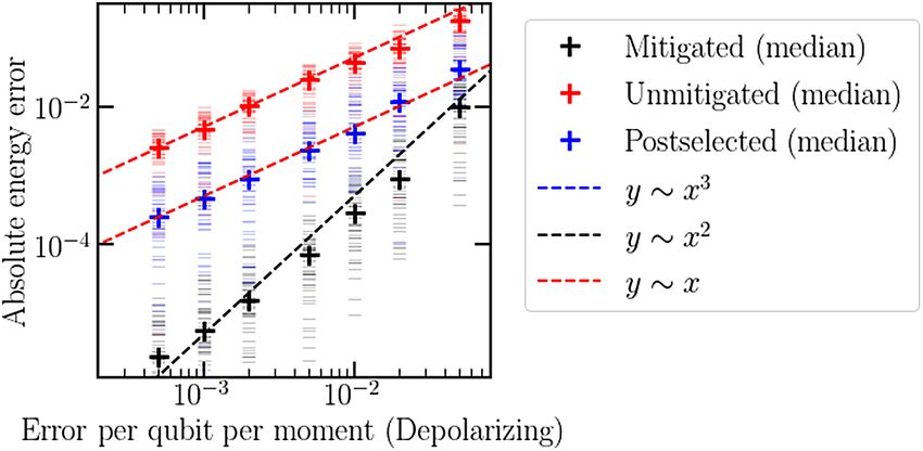
ERROR MITIGATION VIA VERIFIED PHASE...                                                          PRX QUANTUM 2, 020317 (2021)

complicated methods to be found later in the text. The idea             A process diagram for a simplified verified phase esti-
behind all verification protocols is to prepare |ψ = Up |0,          mation protocol is given in Fig. 1. To begin, we write
indirectly estimate H  via phase estimation, and then ver-          H as a sum of fast-forwardable terms Hs (multiplied by
                                                         †
ify that we remain in |ψ by uncomputing |0 = Up |ψ                 coefficients hs )
and measuring in the computational basis. If |ψ is not
an eigenstate of H , the system may by shifted away from
                                                                                                     Ns

this state by the quantum phase estimation unitary—i.e.,                                       H=           hs Hs .                  (1)
                                                                                                      s=1
even in the absence of error we do not expect the system to
always pass verification. However, as we show later in this            Here, by fast forwardable we mean that each Hs is cho-
work, the data required for phase estimation are contained            sen such that time evolution eiHs t may be implemented
entirely within the set of experiments that pass verifica-             on a quantum register with the same number of gates
tion; we may effectively ignore any experiments that fail.             for each value of t. Although fast forwarding is forbid-
This in turn allows us to ignore any errors that knock                den for arbitrary H [37], decomposition of any sparse,
the system away from |ψ, making this a potent error                  row computable H into a linear combination of poly-
mitigation scheme. We have constructed various imple-                 nomially many fast-forwardable Hamiltonians is always
mentations of this idea, which we expand on in Secs. III              possible [38]. For example, the N -qubit Pauli operators
and IV, and compare in Sec. V. However, the most general              Pi ∈ PN = {1, X , Y, Z}⊗N form a basis for the set of all N -
protocols require relatively complicated circuits and classi-         qubit operators and are themselves fast forwardable; we
cal postprocessing. For clarity of exposition, in this section        take this decomposition for our simple example.
we focus on stepping through a simple protocol for the                   We then implement verified phase estimation (with a
verification of expectation values, which avoids complex               single control qubit) to estimate the expectation values
signal processing and circuity requirements. The protocol             ψ|Hs |ψ. This involves evolving the system by Hs con-
we describe will work for arbitrary H and |ψ, and may                ditional on a control qubit. (Circuits to implement this are
often be a desirable choice for a real experiment. How-               well known; see, e.g., Ref. [39].) The conditional evolu-
ever, depending on the choices of H and |ψ and the noise             tion encodes a phase function on the control qubit. That is,
model, other protocols described later in the text may be             if we write Xc and Yc for the X and Y Pauli operators on
more optimal in terms of their mitigation power.                      this control qubit, following the conditional evolution we

FIG. 1. Process diagram of the protocol for verified estimation of the expectation value of a Hamiltonian on a state |ψ = Up |0.
Blue denotes circuits to be executed or data to be extracted from a quantum computer; red denotes signal details to be estimated
via classical postprocessing. The protocol proceeds as follows. Top left: a complex Hamiltonian H is split into a number of fast-
forwardable summands Hs . The spectral function g(t) of | under time evolution of each piece is obtained (bottom left) via verified,
fast-forwarded phase estimation. In this example, a control qubit is used to extract the phase function via phase kickback. The resulting
data form a weighted sum of oscillations with frequencies equal to the eigenvalues Ej(s) of the corresponding factor (bottom middle).
This may be decomposed in a variety of classical postprocessing techniques to obtain estimations of the expectation values Hs
depending on the type of Hs chosen (bottom right). Regardless of the method used, the expectation values must be normalized to obey
Eq. (24), the last step in the verification process. As the expectation value is linear, the verified estimates of Hs  obtained may be
immediately summed together to give a verified estimate for H  (top right).

                                                               020317-3
THOMAS E. O’BRIEN et al. PRX QUANTUM 2, 020317 (2021)
have Note that each Hs will have different values of A0 , A1 , and
g(t) (we have avoided explicitly labeling the above for
Xc + iYc = A0 eit + A1 e−it =: g(t). (2) simplicity). In practice, the number of samples for estima-
Here, A0 and A1 are the squared amplitudes of |ψ in the tion of each Hs should be varied to minimize the error in
eigenbasis of Hs (which has known eigenvalues ±1). The the final estimation of H (i.e., importance sampling on
expectation value Xc may be estimated by measuring the the hs coefficients).
control qubit M times in the x basis, counting the number
of times mx,0 or mx,1 a 0 or 1 is seen, and approximating III. SCHEMES FOR VERIFIED PHASE
ESTIMATION
mx,0 − mx,1
Xc ≈ . (3) A. Review of single-control quantum phase estimation
M
Quantum phase estimation (QPE) refers to a family of
(A similar procedure may be performed for Y.) To verify
protocols to learn eigenphases eiφj of a unitary operator
this estimate, we uncompute the preparation of the system,
U. Equivalently, quantum phase estimation may be used
and count the number m(v) (v)
x,0 (mx,1 ) of measurements of 0 to learn eigenvalues Ej of a Hermitian operator H , as
(1) on the control qubit when the uncomputed state on the
each such operator generates a unitary via exponentiation:
system is returned to the initial |0 state. We then replace
U = eiHt [40]. (Such estimation requires limiting the size
our estimation by iE t
of t to prevent aliasing—eiEj t = e j if Ej t = Ej t + 2nπ ,
m(v) (v)
x,0 − mx,1
which makes estimation ambiguous.) The eigenvalues of
Xc ≈ . (4) H and the eigenphases of U are related by the same expo-
M
nentiation and correspond to the same eigenstates |Ej —if
[Note that we only replace the numerator, and not the H |Ej = Ej |Ej , U|Ej = eiφj |Ej and φj = Ej t.
denominator, of Eq. (3), which makes this not strictly post- In the single-control variant of QPE, the phases φj are
selection; see Sec. III B for more details.] The expectation learnt by imprinting them on a control qubit—a process
value Hs is encoded within the phase function g(t), and known as phase kickback. Any unitary U may be imple-
must be inferred from the estimates above. In our example mented as a (perhaps approximate) quantum circuit on a
protocol, this requires inferring the amplitudes A0 and A1 quantum “system” register, but quantum mechanics tells
(as the eigenvalues ±1 are already known). These may be us that eiφ |ψ ≡ |ψ for all pure states |ψ and numbers
simply estimated by a two-parameter fit of Eq. (2) to the φ ∈ R. This implies that if the system register were pre-
extracted values of g(t). pared in the pure state |Ej and U applied, we would
As we show later in the text, in the absence of error, not be able to infer the phase φj from the resulting state
Eqs. (3) and (4) yield the same result (in the large M eiφj |Ej ≡ √
|Ej . However, a relative phase φ between two
limit). Errors tend to scatter the system into a state that states, (1/ 2)(|ψ1 + eiφ |ψ2 ), is a physical observable
fails verification. The primary effect this has on the estima- that may be detected. Such detection may be achieved by
tor in Eq. (4) is to rescale g(t) → pNE g(t) (where pNE is performing the unitary U conditional on the control qubit
the probability of no error occurring). However, the con- being in the state |1 (and doing nothing when the control
verse is not true; states may fail verification due to the qubit is in the state |0). This is commonly written as the
relative dephasing between the |0 and |1 eigenstates of “controlled” unitary C − U. When C − U acts on a sys-
Hs , and we cannot infer the value of pNE from a single tem register prepared in an eigenstate√|Ej and a control
point g(t). Instead, we can infer the value of pNE from the qubit prepared in the state (|0 + |1)/ 2, the global state
normalization of the starting state |ψ. As our circuit is evolves to
fast forwarded, under reasonable noise assumptions, pNE is
independent of t, and this propagates immediately through 1 1
the fit of Eq. (2): A0 , A1 → pNE A0 =: Ã0 , pNE A1 =: Ã1 . C − U √ (|0 + |1)|Ej = √ (|0 + eiφj |1)|Ej . (7)
2 2
The normalization of |ψ requires A0 + A1 = 1, and we
may correct for this by estimating
We see that the eigenphase eiφj from the system register
Ã0 − Ã1 is kicked back onto the control qubit, while the system
Hs = . (5) register itself remains unchanged. We may estimate this
Ã0 + Ã1
eigenphase eiφj by repeatedly performing the QPE proto-
Finally, as expectation values are linear, after repeating this col, measuring the control qubit in the X or the Y basis, and
procedure for all Hs in Eq. (1), we may sum the result; recording the number of single-shot readouts of 1 and 0. In
the Hamiltonian case, from this estimate one may immedi-
H = hs Hs . (6) ately infer that (1/it)Arg(eiφj ) = Ej mod 2π t. The error
s in the estimation of Ej decreases with t; asymptotically
020317-4ERROR MITIGATION VIA VERIFIED PHASE... PRX QUANTUM 2, 020317 (2021)
optimal protocols need to balance this against the ambi- y basis, reading it out, and averaging the output over many
guity modulo 2π t by repeating the estimation at multiple repetitions (or shots) of the experiment.
values of t [41–43]. In terms of estimating the eigenphases For a unitary operator U, one may obtain an equivalent
eiφj of a unitary U, this optimization requires repeating the phase function
above procedure for C − Uk at varying points k.
Often, one does not prepare an eigenstate |Ej , but g(k) = Aj eikφj (14)
instead prepares a starting state j
|ψs = aj |Ej . (8) by estimating
j
g(k) = 2Tracec [ρc (k)|01|]
Applying C − Uk to such a state no longer leaves it = Tracec [ρc (k)X ] + iTracec [ρc (k)Y], (15)
unchanged, but instead entangles it with the control qubit.
This produces the combined state (on the system+control
register) ρc (k) = Tracesys [|(k)(k)|], (16)
1
|(k) = C − Uk √ (|0 + |1)|ψs with |(k) defined in Eq. (9). The tomography to extract
2 these expectation values is the same as described in the
aj previous paragraph.
= √ (|0 + eikφj |1)|Ej . (9)
2 Information about the eigenvalues Ej and amplitudes
j
Aj = |aj |2 may be inferred classically from estimates of
When one has instead performed controlled time evolution g(t) at multiple values of t. When these are estimated suffi-
(via the unitary C − eiHt ), one may instead write ciently well, the expectation value of the Hamiltonian may
be calculated as
1
|(t) = C − eiHt √ (|0 + |1)|ψs H = Aj Ej . (17)
2
j
1
= aj √ (|0 + eiEj t |1)|Ej . (10)
2 Inference of the amplitudes Aj from g(t) to error takes
j
asymptotic time ( −2 ) on a quantum device, even when
The sum over j in the above equation looks problematic, the eigenvalues Ej are already known [44]. By propagating
but it turns out that the eigenphases φj (or eigenvalues Ej ) variances, this implies equivalent convergence in the esti-
remain encoded on the control qubit, in a sum weighted by mation of expectation values via Eq. (17). One need not
the norm square Aj := |aj |2 of the initial amplitudes aj . To resolve all 2N eigenvalues of an N -qubit operator in order
be precise, one may trace over the system register to obtain to evaluate Eq. (17). Time-series analysis methods [34] or
the reduced density matrix of the control qubit integral methods [45] produce a coarse-grained approxi-
mation to the spectrum that may be averaged over to obtain
ρc (t) = Tracesys [|(t)(t)|] (11) expectation values with similar convergence rates. Alter-
natively, for simple operators with a highly degenerate
1 1 g(t) spectrum (e.g., Pauli operators), curve fitting will be suf-
= ∗
2 g (t) 1 ficient to extract the required data (as described in Sec. II)
[46].
with g(t) the phase function of |ψs under H ,
B. Verifying a phase estimation experiment
g(t) = Aj eiEj t . (12) As the data from single-control quantum phase estima-
j
tion are accumulated entirely on the control qubit, one
would be tempted to throw the system register away (or
Estimates of g(t) may be obtained as an expectation value rather, reset the register and begin anew). In the absence of
error correction this temptation grows larger; noise levels
g(t) = 2Tracec [ρc (t)|01|] in near-term devices are high enough that coherent states
= Tracec [ρc (t)X ] + iTracec [ρc (t)Y] (13) of more than a few qubits degrade over the course of any
reasonably sized algorithm to within a few percent fidelity
of the Pauli operators X and Y. Measuring these expecta- to the target state—if not less [4]. However, even when
tion values requires rotating the control qubit into the x or corrupted, the information contained within the system
020317-5THOMAS E. O’BRIEN et al. PRX QUANTUM 2, 020317 (2021)
register is valuable, as one can use this information to diag- Note that postselecting (i.e., keeping only the experimental
nose potential errors in the data to be read from the control data where verification was passed) would instead prepare
qubit. For instance, in the presence of global symmetries of the state ρc(v) /Trace[ρc(v) ]. This will not yield the desired
the Hamiltonian, one could imagine mitigating errors that result, as
do not commute with this symmetry via symmetry verifi-
cation [29,30,32]. In verifying these symmetries, we are in Trace[ρc(v) (X + iY)] g(t)
effect projecting the system into a subspace of the global = , (21)
Trace[ρc(v) ] 1 + |g(t)|2
Hilbert space that contains the information we desire. One
could imagine constructing ever-smaller Hilbert spaces,
which trades circuit complexity for error-detection power. which is not equal to g(t) unless |ψs is an eigenstate of eiHt
It turns out that the limit of this construction is achievable: (in which case ρc(v) = ρc ). (Moreover, this rescaling can be
instead of measuring one or more symmetries on the sys- up to a factor 2 in the absence of noise, and the spectrum of
tem register, we can instead verify that it has returned to its this new function is significantly different to the original.)
initial state |ψs . (This is similar to the echo-type measure- To give some intuition, one can imagine phase estimation
ments made in randomized benchmarking [47] or quantum on a mixed state in two steps: performing phase estimation
Hamiltonian learning [48].) on individual states to generate a set of signal functions
Assuming that |ψs is prepared from the computational eiEj t , and then summing and returning the weighted result
basis state |0 by a preparation unitary Up , this measure- g(t). The set of states that fail verification, ρ (f ) , captures
† the relative dephasing between these states, which cannot
ment may be achieved by applying Up , and reading out
be ignored when attempting to recover this result. Instead,
each qubit in the computational basis. One would expect
an explicit protocol for the measurement of a single g(t)
such a measurement to distort the phase function g(t), but
within verified single-control phase estimation takes the
this is not so, as we may expand the trace in Eq. (11) to
following form.
show that
Tracec [ρc (t)|01|] = Tracec [ψs |(t)(t)|ψs |01|]. †
(18) Inputs: circuits to implement Up , Up and controlled time
evolution eiHt ; number of repetitions M of measurements
Here, the left-hand side of the equation is the expectation in the x and y bases.
value of ρc (t) regardless of the state of the control register, Output: an estimate of g(t) with variance O(1/M ) in both
and the right-hand side is the (non-normalized) expecta- the real and imaginary parts.
tion value of ρc (t) on verified experiments only. The lack
of normalization means that this is not a postselection tech- 1. Prepare classical initial variables g x = 0, g y = 0.
nique; instead one assumes that the contribution of states 2. Prepare the system register in a starting state
that fail verification to the final estimation of g(t) is zero. |ψs √= Up |0 and the control qubit in the state
[By contrast, states that pass verification either contribute (1/ 2)(|0 + |1).
+1 or −1 to the estimation of g(t).] 3. Simulate time evolution eiHt conditional on the con-
We can make a physical argument why Eq. (18) holds trol qubit.
†
and verification should not affect the estimation of g(t) in 4. Apply the inverse circuit Up to the system register.
the absence of noise. Let us decompose the reduced density 5. Rotate the control qubit into the X or Y basis and
matrix on the control qubit as measure it to obtain a number m ∈ [0, 1].
6. If all qubits in the system register read 0, increment
ρc = ρc(v) + ρc(f ) , (19) the relevant variable g x or g y by (−1)m .
7. Repeat steps 2–6 M times in the X basis and M
i.e., into the ensemble of states that have passed verifica- times in the Y basis, and estimate g(t) by g x /M +
(f )
tion, ρc(v) , and those that have failed, ρc . When the control ig y /M .
qubit is in the |0 state, the system register is not evolved,
so in the absence of noise the state will pass verification Algorithm 1. Single-control VPE.
every time. This implies that a verification failure in the
absence of noise projects the control qubit into the |1 state; We consider the increased sampling cost in the presence
(f ) of error in Sec. III C 1.
ρc = |11|. As Trace[|11|01|] = 0, this fraction of
states on average contributes nothing to the estimate of
g(t). In other words, C. Why verification mitigates errors
The mitigation power from verification is based on the
Trace[ρc |01|] = Trace[ρc(v) |01|] = g(t). (20) relative size of the Hilbert spaces in which the states that
020317-6ERROR MITIGATION VIA VERIFIED PHASE... PRX QUANTUM 2, 020317 (2021)
have passed verification and states that have failed ver- The above analysis is not necessarily true for simulation
ification, ρ = ρ (v) + ρ (f ) , live. If we define the Hilbert of an arbitrary Hamiltonian under a realistic noise model.
spaces in which the two ensembles live H(v) and H(f ) , In particular, if the instantaneous state during simulation
respectively, we have dim[H(v) ] = 2, while dim[H(f ) ] = is a near eigenstate of the error model, then the correction
2N +1 − 2. An error that occurs during the circuit is then in Eq. (22) may be as large as O(1) instead of O(2−N ).
likely to scatter the system into the set of rejected states. As In Appendix A we study this in more detail, and specify
an extreme example, the probability that a completely ran- the conditions under which errors will distort the results of
dom error (i.e., an error that scatters all states to a random verified phase estimation.
state) at any point in the circuit will yield a state in H(v)
can be immediately calculated to be 2/(2N +1 − 2) ∼ 2−N . 1. Sampling costs
This includes errors during preparation of |ψs by the uni-
† The error mitigation from verification comes at the cost
tary Up and the inversion of Up to perform the verification of increasing the number of samples required to estimate
itself. As we are not postselecting on the verification out- g(t). Assuming that all errors fall outside the verified sub-
put, g(t) is still affected by this shift, but the distortion may space, estimating g(t) to precision requires estimating
be accounted for in classical postprocessing. In this sim- gerr (t) to precision pNE . To obtain g x in Algorithm 1 (and
ple noise model the effect of noise is then to replace the equivalently for g y ), we average over a set of M experi-
estimate of g(t) by mental outputs that may take the values {−1, 0, 1}. Let us
gerr (t) = pNE (t)g(t) + O[2−N perr (t)], (22) define the ith experimental output gix ; then we have
where pNE (t) and perr (t) are the probabilities of no error P(gix = ±1) = 12 pNE (1 ± g x ), (27)
or some error occurring, respectively. (In Appendix A we
P(gix = 0) = 1 − pNE . (28)
derive the specific requirements for this to be the case.)
Assuming that errors occur at a constant rate as a function
Our estimate of the noisy gerr (t) is then given by
of the circuit depth, and all scatter the system outside H(v) ,
for fast-forwardable Hamiltonians, pNE (t) = pNE and
Re[gerr (t)] = P(gix = 1) − P(gix = −1). (29)
gerr (t) = pNE g(t) = (pNE Aj )eiEj t . (23)
j
As each experiment is independent and identically dis-
tributed, the variance on our estimates of these probabil-
This can be seen as a uniform damping of each squared ities is
amplitude Aj to Aj = pNE Aj . Such damping may be cor-
rected for classically as we know |ψs is normalized, Var[P(gi = ±1)] =
x 1 1 1
pNE (1 ± g ) 1 − pNE (1 ± g ) ,
x x
M2 2
Aj = 1, (24) (30)
j
and so we may estimate
1 2
Cov[P(gix = 1), P(gix = −1)] = − p (1 − [g x ]2 ).
Aj 4M NE
Aj = . (25) (31)
j Aj
Depending on the classical signal processing method used, Propagating variances gives
one may not obtain estimates of all Aj and Ej , but may
1 1 2 x 2
instead directly calculate j Aj Ej and j Aj . For exam-
Var{Re[gerr (t)]} = pNE − pNE [g ] . (32)
ple, one could use gerr (0) = j Aj as such a reference M M
point. For non-fast-forwardable Hamiltonians, assuming We may then bound the requirements to estimate gerr (t) to
again that errors occur at a constant rate throughout the −2
variance −2 pNE by
circuit and that all scatter the system outside H(v) , we have
−1
M ≥ −2 pNE . (33)
gerr (t) = e−t/τerr g(t) = Aj ei(Ej +i/τerr )t . (26)
j
This is exactly what one would expect from an actual post-
This can be seen to be an imaginary shift to the eigenvalues selection technique [i.e., where MpNE samples are used to
Ej → Ej + iτerr . It can be corrected for in signal process- estimate g(t)]. We remind the reader that pNE here is the
ing of the phase function by taking only the real parts of probability of no error occurring over the entire circuit.
the Ej eigenvalues. As one should expect for an error mitigation technique,
020317-7THOMAS E. O’BRIEN et al. PRX QUANTUM 2, 020317 (2021)
this in turn grows exponentially with the size of the cir- may be required to unbias the estimate of g(t). An example
cuit required to implement eiHt or Up . In a simple model, of this biasing effect is if an amplitude-damping channel
if the error per qubit per moment is p (i.e., assuming qubit
decay is more dominant than gate noise in the model), an λ
Rampdamp [ρ] =(1 − λ)ρ + (Z + I )ρ(Z + I )
N -qubit circuit of depth d would have 2
λ
+ (X + iY)ρ(X − iY) (39)
pNE = (1 − p)Nd , (34) 2
is present on the control qubit between the final measure-
and thus the number of shots required to estimate (the real ment prerotation and readout in the computational basis.
or imaginary part) of g(t) would scale as Left unchecked, this will shift the estimate of g(t) to
M ∼ (1 − p)−Nd −2 . (35) gerr (t) = (1 − λ)g(t) + λ. (40)
This is not to be ignored; verification requires at least dou- In addition to damping the true signal g(t), this additive
bling the size of the circuit, which, if pNE = 0.01 (as has signal presents as a 0-energy eigenvalue in the spectrum
been reported [1] and mitigated successfully [4] in previ- of g(t). This will not be accounted for by naive renormal-
ous experiments), will increase the measurement count by ization of H as outlined in Algorithm 3 below; the esti-
a factor of 100. Some of the methods presented in this work mation protocol will instead estimate (1 − λ)H . Though
involve increasing the circuit depth by factors of up to 14, this could be corrected in postprocessing, we suggest that a
which will be impractical for large experiments without more stable mitigation is to flip the |0 and |1 states on the
further circuit optimization. control qubit for half of the experiments. This may be com-
piled into the final prerotation, and does not increase the
total sampling cost of the experiment (only half as many
2. Control noise samples need to be taken at each prerotation setting for
An important realistic error to consider in QPE is error the same accuracy). We observe similar biases on bit-flip
on the control qubit. This keeps the system within the noise channels that tend to decay the real and imaginary
verified subspace, and so is not captured by the above anal- parts of g(t) asymmetrically. This may be compensated
ysis. However, the effect of many common error channels for in turn by compiling a π/4 Z rotation on the initial
may still be mitigated by verification. For example, let us control qubit state, and uncompiling it in the final prerota-
assume that the circuit decomposition of C − U involves tion. (One can see that this commutes with all gates in
the control qubit performing only single-qubit gates and the circuit.) For the noise models studied numerically in
controlled operations on the rest of the circuit (which is this text, we have found either one or both of the above
typically the case). In this case, one may show that the compilation schemes sufficient to mitigate control error.
effect of a depolarizing channel of strength λ, More complicated noise models may require more com-
plicated compilation schemes; extending the above will be
3λ λ an interesting task for future work. In particular, the above
Rdepol [ρ] = 1 − ρ + (X ρX + YρY + ZρZ), analysis does not apply to correlated two-qubit noise dur-
4 4
(36) ing operations between the control qubit and the rest of the
system.
acting on the control qubit at any point in the circuit, sends
the final state of the system to D. Verified control-free phase estimation
As was recently demonstrated in Ref. [35], the con-
(1 − λ)ρNE + λρerr , (37) trol qubit may be removed from a QPE experiment if
we have the ability to prepare an alternative reference
eigenstate |ψr of the Hamiltonian H (with ψs |ψr = 0).
where ρNE is the state in the absence of error, and
For example, in the electronic structure problem in quan-
tum chemistry the number-conserving Hamiltonian has the
Trace[ψs |ρerr |ψs |01|] = 0. (38) vacuum as a potential reference state. (A similar situation
was considered in Ref. [50] for the purposes of random
In this case, the (noisy) estimate of g(t) is sent to (1 − gap estimation, but estimating single eigenvalues Ej from
λ)g(t), and expectation values and eigenvalues may be this class of experiments is somewhat awkward.) This was
recovered via the same analysis as in Sec. III C. However, also recently considered as an extension to the well-known
the above analysis will not hold for a more general noise robust QPE scheme [51], requiring both |ψr and |ψs to
model, and schemes such as randomized compiling [49] be eigenstates of the system [36]. Note that |ψr need not
020317-8ERROR MITIGATION VIA VERIFIED PHASE... PRX QUANTUM 2, 020317 (2021)
Inputs: circuits to prepare a superposition of |ψs and |ψr ,
invert the preparation, and implement time evolution eiHt ;
number of repetitions M of measurements in the x and y
bases; the reference eigenstate energy Er .
FIG. 2. Quantum circuit for control-free verified phase estima- Output: an estimate of g(t) [Eq. (41)] with variance
tion. The preparation unitary Up is defined in Eq. (42). The first O(1/M ) in both the real and imaginary parts.
gate in the circuit is a Hadamard gate (roman H) on the top-most
qubit (labeled the target qubit in the text), which should not be 1. Prepare classical initial variables g x = 0, g y = 0.
confused with the Hamiltonian H . 2. Prepare the system register √in a starting state
√
(1/ 2)(|ψs + |ψr ) = Up (1/ 2)(|0 + |1T ).
necessarily be a zero-energy eigenstate of H , though the 3. Apply the unitary Uk (or, equivalently, simulate time
corresponding eigenenergy Er should be known to high evolution eiHt ).
†
accuracy.√In this case, one needs to prepare the correlated 4. Apply the inverse circuit Up to the system register.
state (1/ 2)(|ψs + |ψr ) and perform uncontrolled time 5. Rotate the target qubit into the X or Y basis and
evolution, and finally measure the off-diagonal element measure it to obtain a number m ∈ 0, 1.
|ψs ψr |. This is shown in the circuit (Fig. 2). Evaluating 6. Measure all other qubits, and if they all read out 0,
the circuit provides an estimate of increment the relevant variable g x or g y by (−1)m .
7. Repeat steps 2–6 M times in the X basis and
Trace[U(|ψr + |ψs )(ψr | + ψs |)U† |ψr ψs |] M times in the Y basis, and estimate g(t) by
eiEr t (g x /M + ig y /M ).
= e−iEr t g(t), (41)
and the additional phase may be subtracted in postprocess- Algorithm 2. Control-free VPE.
ing.
The protocol for verified control-free phase estima-
tion does not differ significantly from the single-control The analysis of Sec. III C is identical for the control-free
case. Besides the loss of the control qubit and removal case, with the absence of the issue of control noise, as is the
of control from the time evolution circuit, we also now analysis of Sec. III C 1. However, we note that at the begin-
require ning and the end of any experiment, single-qubit noise on
√ our preparation circuit to prepare the starting state the target qubit behaves similarly to control qubit noise.
(1/ 2)(|ψs + |ψr ). We assume that this is achieved by
first applying a Hadamard gate to a single target qubit This necessitates averaging over multiple initial and final
in the rotations of the target qubit to prevent bias in the estimation
√ system register, placing the system in the state of g(t).
(1/ 2)(|0 + |1T ). (Here we use the notation |1T for the
basis state where the target qubit is in the |1 state and all The above analysis implies that the algorithms studied
other qubits are in |0.) Then, the desired preparation may in Refs. [35,50] should be amenable to verification imme-
be achieved by a preparation unitary Up that performs the diately as well. It also provides some additional explana-
mapping tion for the error robustness observed in the robust phase
estimation of Ref. [36].
Up |0 → |ψr , Up |1T → |ψs . (42)
IV. VERIFIED EXPECTATION VALUE
ESTIMATION
(We use the same notation as for the single-control unitary
on purpose, as, under the associations |0|ψs ↔ |ψr and In many circumstances, one wishes not to know the
|1 ↔ |ψs , one may see that the two are equivalent.) With eigenvalues of a Hermitian operator H , but instead its
this definition, estimation of |ψr ψs | may be achieved by expectation value H under a specified state |. For
inverting Up , as instance, in a variational quantum eigensolver [18], one
prepares a state |(θ) = U(θ)|0 dependent on a set of
classical input parameters θ, then measures the expec-
|ψr ψs | = Up |01T |U†p . (43) tation value E(θ) = (θ)|H |(θ). This is then opti-
mized over θ in a classical outer loop, with the optimized
In particular, after inversion, the reduced density matrix of state |(θopt ) hopefully a good approximation of the true
the target qubit contains the desired phase function g(t), ground state |E0 . In quantum variational algorithms it is
and the verification consists of checking whether all other typical that (θ)|H |(θ) is estimated by means of par-
qubits are measured into 0. The full control-free protocol tial state tomography [31,52,53]. However, noise in the
is then the following. preparation unitary U(θ) causes an errant state ρerr (θ)
=
020317-9THOMAS E. O’BRIEN et al. PRX QUANTUM 2, 020317 (2021)
|(θ)( to be prepared and tomographed, propagat-
θ)| This can be seen to be the Fourier transform of the phase
ing the preparation error directly to a final estimation error. function g(t) [strictly, g(t) is the inverse Fourier trans-
The noise analysis in Sec. III C extends to both the prepara- form of gS (E/2π )], and a coarse-grained approximation
tion and mitigation unitaries, so if verified phase estimation may be obtained via time-series methods [34] or integral
is used to provide estimates of eigenvalues and amplitudes, methods [45] with rigorous bounds on each. Numerically,
one may reconstruct we find that signal processing methods such as Prony’s
method [33] also perform acceptably (see Sec. V D). For
|(θ)
(θ)|H = |aj |2 Ej , (44) fast-forwardable Hamiltonians (such as Pauli operators),
j one often already knows the target eigenvalues of the
problem. Furthermore, the eigenspectrum of these Hamil-
and inherit the mitigation power of the verification proto- tonians is often highly degenerate, making simple curve
col. This has the added advantage that control errors in the fitting a practical (and attractive) alternative.
preparation circuit (which, being a repeated error, are not Instead of analyzing the phase function at many points
mitigated against) are able to be compensated for during as described above, one may expand
the outer optimization loop of the VQE, as is well known
[4,18]. Quantum phase estimation has previously been sug- Im[g(t)] = |aj |2 sin(Ej t)
gested as an alternative to partial state tomography for j
expectation value estimation, both to improve the rate of 1
estimation [54] and to provide a witness for the presence =t |aj |2 Ej + t3 |aj |2 Ej3 + O(t5 ), (47)
of eigenstates of the Hamiltonian [55]. The verification j
3 j
protocols described in this work should be applicable to
these methods as well. A general algorithm for verified
expectation value estimation takes the following form. 1
Im[g(t)] = (θ)|H |(θ) + O(t2 ), (48)
t
†
Inputs: (noisy) circuits to implement Up , Up and con- and simply estimate Im[g(t)] for short times t. This is simi-
trolled time evolution eiHt ; a set of t values; number of rep- lar to the manner in which eigenphases are estimated in the
etitions M of measurements in the x and y bases (that can WAVES protocol [55] (sans verification). In this case, the
be t dependent); a method for classical signal processing normalization of the resulting amplitudes [Eq. (25)] must
(e.g., a curve fitting algorithm). be achieved by the condition that g(0) = j Aj , yielding
Output: an estimate of H .
Im[gerr (t)]
1. Estimate gerr (t) for all given points t using H = + O(t2 ). (49)
t|gerr (0)|
Algorithm 1 to the chosen precision.
2. Obtain estimates for individual Ej and Aj values via A. Fast-forwarded and parallelized Hamiltonian
classical signal processing. decompositions
3. Estimate H as
As expectation values are linear, we may estimate H
by splitting it into multiple terms, estimating the expecta-
j Aj Ej
H = . (45) tion values of each term individually, and resumming:
j Aj
H= Hs → H = Hs . (50)
Algorithm 3. Verified expectation value estimation. s s
If individual Hs may be simulated at a lower circuit depth,
One might worry that the sum in Eq. (44) is over an this can reduce the accumulation of unmitigated errors, at
exponentially large number of eigenstates |Ej . However, the cost of requiring more simulation. This ability becomes
one need not resolve all eigenvalues Ej in order to accu- especially useful if one chooses the Hs to be fast forward-
rately estimate the expectation value (θ)|H |(θ); if able. Here, we define a fast-forwardable Hamiltonian Hs
eigenvalues within δ of each other are binned, the resulting as one for which a circuit implementation of eiHs t has con-
expectation value will be accurate to within δ. We may for- stant depth in t. The circuit depth required to simulate eiHt
malize this by considering the spectral function gS of |ψs for arbitrary H is bounded below as O(t) [37], but, for cer-
under H , tain operators, this may be improved on [56]. For example,
as the Pauli operators {1, X , Y, Z}⊗N are both fast forward-
gS (E) = Aj δ(E − Ej ). (46) able and form a basis for the set of N -qubit Hermitian
j operators, a set of Hs terms may be taken from these to
020317-10ERROR MITIGATION VIA VERIFIED PHASE... PRX QUANTUM 2, 020317 (2021)
decompose an arbitrary Hamiltonian. As another exam- in a real experiment to choose the best mitigation tech-
ple, given an instance of the electronic structure problem, nique (or combination of mitigation techniques) for the
one may attempt a low-rank factorization of the interac- job. Though a comparison between multiple techniques in
tion operator into a sum of O(N ) diagonalizable (and thus a realistic setting lies outside the scope of this work, we
fast-forwardable) terms [57]. give some predictions here on how VPE might compare in
In order to speed up estimation of expectation val- performance to other mitigation techniques, and whether it
ues ofmultiple terms Hs in a decomposed Hamiltonian might be possible to compare to different techniques. We
H = s Hs , it may be possible to perform the verified can classify all error mitigation techniques that the authors
phase estimation step of each Hs in parallel. For example, know of into the following broad categories.
we can perform time evolution of L multiple summands,
each controlled by a different control qubit, in between the (a) Circuit design: many forms of noise may be miti-
preparation and verification steps of a single instance. In gated by careful design of a circuit to, e.g., minimize
the absence of verification, such parallelization will not crosstalk between simultaneous gates [58], cancel
affect the outcome of quantum phase estimation of any out Z over- or under-rotation (e.g., via echo pulses
individual Hs , so long as all terms estimated in parallel [59]), or optimize a circuit variationally to can-
commute. This follows immediately from the fact that the cel out control parameter drift on a long timescale
time evolution for one such term does not evolve the sys- [18,60]. (Whether or not this counts as error mitiga-
tem between eigenspaces of another. This is complicated tion or calibration of the underlying quantum device
by the addition of verification, as the additional circuitry is left to the reader to decide.) Depending on the
means that the system may evolve away from |ψs despite source of noise these techniques may significantly
a specific control qubit being in |0. In Appendix B, we reduce or even nullify its effect, which may be far
show that this gives rise to a set of spurious signals in the more effective than VPE. On the other hand, noise
estimated phase function g (s) (t): sources such as T1 error cannot be easily calibrated
away (due to the associated photon loss); in these
(s) situations (where VPE performs quite well) these
Bj(s),j e
iF t
gq(s) (t) = v,j ,j . (51) methods will have little effect. VPE is clearly com-
v,j ,j patible with any such techniques, as these consist of
adjustments to the implementation of a given circuit
Here, the ghost eigenvalues are rather than an algorithmic overhead.
(b) Postselection or verification techniques: this class
(s) (s)
Fv,j ,j = Ej + vs (Ej(s) − Ej(s ) ), (52) of techniques uses knowledge of the problem to
s =s restrict the state of the quantum device to within
a small region of the N -qubit Hilbert space, often
by leveraging symmetries of the Hamiltonian of the
where the Ej(s ) are the true eigenvalues of the Hamiltonians
problem to be solved. VPE itself falls into this cate-
Hs and v is an L-bit vector written in binary (i.e., vs ∈ 0, 1).
gory, alongside symmetry verification [29,30], and
The corresponding, v-independent amplitudes are
quantum subspace expansion techniques [23,24].
1 The performance of these techniques is dependent
Bj ,j = Aj Aj . (53) on their ability to catch errors outside the allowed
2L Hilbert space, so, as the dimension of the Hilbert
Although this is a far more complicated signal than the space for VPE is only 2, we expect it to have greater
standard phase function g(t), we calculate in Appendix B mitigation power in general than these other tech-
that it yields the same expectation value, i.e., niques. (This can be observed in Appendix G, where
VPE shows an asymptotic improvement over sym-
(s) metry verification in a small numerical simulation.)
Bj ,j Fv,j ,j = Hs . (54) However, as the circuit depth of VPE is typically
v,j ,j
far longer than that of other postselection or verifi-
cation techniques (which can be achieved in some
This implies that verified parallel phase estimation may cases without any additional circuitry), the require-
proceed in much the same way as the series protocol. ments on the number of measurements to overcome
sampling noise will be significantly worse. As these
B. Comparison to other methods of error mitigation techniques overlap in their effect on the quantum
Error mitigation techniques differ vastly, both in their state, it is not particularly possible to combine them;
cost to implement and their effectiveness against different instead one should choose the best trade-off between
forms of noise. This implies that care needs to be taken mitigation power and the number of measurements.
020317-11THOMAS E. O’BRIEN et al. PRX QUANTUM 2, 020317 (2021)
(c) Error extrapolation techniques: assuming that one (f) Purification techniques: as the output of a quan-
can artificially introduce noise into a system, these tum algorithm is often ideally pure, these techniques
techniques rely on parameterizing the output f of a attempt to reduce errors by mapping a noisy impure
quantum circuit as a function of a “noise parameter” state to a purer one. This may be achieved, e.g., for
f = f (λ), fitting a functional form, and extrapo- free-fermion states via McWeeny purification [4], or
lating to λ = 0. The noise parameter can either be for more general states via virtual distillation [64].
adjusted experimentally (e.g., by adjusting the wait For more complex states, the McWeeny process
time or detuning of an underlying gate) [25,27] or cannot be used, but it has proven remarkably effec-
algorithmically (e.g., by inverting noisy gates [61]). tive when available. Virtual distillation and VPE
The mitigation power of such a technique depends appear to be remarkably similar in their increased
on how well the noise can be tuned as a function measurement cost and their mitigation performance,
of this single parameter, and how well one can pin as well as their circuit structure. Understanding this
down a functional form for f (λ). This is not eas- similarity and comparing the two in more detail is a
ily comparable to VPE, as the physical source of clear avenue for future research.
the mitigation is qualitatively significantly different.
We expect that the relative performance will depend V. NUMERICAL EXPERIMENTS
on the experiment and the hardware itself. In the-
ory these methods could be combined with VPE To investigate the mitigation capability of verified phase
(either by extrapolating the phase function or the estimation, we first use it for expectation value estima-
VPE result). However, it is unclear whether the out- tion. To prepare states, we take different variational ansätze
put of VPE will be more challenging to fit, reducing with randomly drawn parameters. We compare the perfor-
the effectiveness of the extrapolation. mance of verified and unverified circuits across multiple
(d) Result extrapolation techniques: instead of fitting target Hamiltonians, noise strengths, and noise models to
the output f of a quantum circuit to an artificial attempt to identify trends in the method. All simulations
noise term, one can consider comparing the output are executed using the Cirq quantum software develop-
of similar quantum circuits tailored to efficient clas- ment framework [65] and simulators therein. Hamiltonians
sical simulation. This technique has been demon- and complex circuits are further generated using code from
strated experimentally in Refs. [58,62], and pro- the OpenFermion [66] libraries. Except for when men-
posed within a VQE setting (by tuning the param- tioned, the Cirq noise models are chosen to be a constant
eters to points where the solution is known) [63]. error rate per qubit per moment, where a moment is a
In some sense VPE can be considered to be simi- period of the circuit where gates occur. Equivalently, this
lar to these methods, with the |ψs |0 or |ψr states can be thought of as an error rate per qubit per gate, but
providing an entangled reference state for the target including error on idling gates as well. The noise models
evolution. However, this relationship is not com- considered are not as complex as those typically observed
pletely clear, as VPE strictly relies on the coherence in experiment (which are typically highly nonuniform,
between the two states. Understanding this similar- and can include crosstalk and non-Markovianity alongside
ity is a clear avenue for future research. Regard- other effects), but we expect our results should provide a
less, VPE should be able to be combined with at suggestion of the mitigation power of this method in a real
least some of these techniques to provide yet more quantum device.
mitigation power.
(e) Probabilistic cancelation techniques: given knowl- A. Givens rotation circuits for free-fermion
edge of the true process maps of the gates being Hamiltonians
performed on a quantum device, one can in prin- We first test the mitigation ability of the verification
ciple construct families of quantum circuits that, protocol on an instance of a “Givens rotation circuit” of
when combined, yield a target noiseless result [25, the form developed for implementing rotations of single-
27]. However, these methods require much addi- particle fermionic basis functions in Ref. [67]. This circuit
tional characterization of the device, which is a takes the form
problem in systems with large amounts of drift.
In principle, given sufficient knowledge of the
U(θ) = exp i θj ,l cj cl ,
†
noise, this method works perfectly, but at a greatly (55)
increased measurement cost, making it difficult to j ,l
make a fair comparison in a theoretical setting.
†
Testing this method against VPE in a real exper- where cj and cj are the creation and annihilation operators
iment would be an interesting target for future for a fermion on site j , and θj ,l = θl,j . Such a circuit is clas-
research. sically simulatable, but it is a critical piece of infrastructure
020317-12ERROR MITIGATION VIA VERIFIED PHASE... PRX QUANTUM 2, 020317 (2021)
in quantum computing applications for quantum chemistry U(θ ) and implement this in a single Givens rotation
[4,11,13,31,57]. It is also low depth: it may be decomposed circuit.
exactly by a sequence of matchgates [68], with optimal The complete VPE circuit for this circuit consists of
compilation in a circuit depth of exactly N . When acting the GHZ preparation, a single Givens rotation, a set of
Nf −1
on a N -qubit register prepared in the state n=0 Xn |0, single-qubit z rotations, uncomputing the Givens rotation,
this may prepare an arbitrary ground state of a free-fermion uncomputing the GHZ preparation, and measurement in
Hamiltonian with Nf particles by an appropriate choice of the X or Y basis. The resulting circuit for verified phase
θ. In this work, we take a simple free-fermion Hamiltonian estimation is more than twice the length of the circuit
as an example—namely, a one-dimensional chain required for the unmitigated VQE. We assume here that
† the VQE tomography does not require any additional over-
H = −t cj cj +1 + H.c. (56) head, and directly estimate the expectation value from the
j simulated density matrix. For verified phase estimation,
we extract the phase function from the simulated density
Such a Hamiltonian may be diagonalized, matrix, and then process it to estimate expectation val-
ues using Prony’s method. In order to not bias the final
H = V† α c†α cα V, (57) readout (which can lead to significant error in estimation),
α we average the rotation into the X and Y bases over both
+π/2 and −π/2 rotations (see Sec. III C 2). To simplify
where V here takes the same form as in Eq. (55). This
the analysis here, we do not include additional sampling
decomposition allows immediately for the fast forwarding
noise. In Fig. 3, we plot the rms error for two error mod-
of time evolution, as
els over a range of noise models and strengths. For each
† noise model and at each strength, we sample 50 random
eiHt = V† eit α α c α c α V choices for the initial parameters θ [and set t = 1 in Eq.
†
= V† eitα cα cα V. (58) (56)]. In the presence of a uniform single-qubit depolar-
α
izing channel (Fig. 3, left), we see that the verified error
displays a clear ∼ p 2 trend (where is the error in the
As the Givens rotation circuits conserve particle number, final estimation and p is the error per qubit per moment).
the vacuum |0 may be used as a reference state for control- This implies that the effect of all single errors in this noise
free verified estimation. A superposition of this reference
Nf
state and starting state U(θ) n=1 Xn |0 may be prepared
by acting the Givens rotation circuit on the Greenberger-
Horne-Zeilinger (GHZ) state
Nf
1
|ψGHZ = √ |0 + Xn |0 , (59)
2 n=1
which may itself be prepared by, e.g., a chain of controlled-
NOT (CNOT) gates:
(rms)
1
(rms)
|ψGHZ = CNOTj −1,j H0 |0. (60)
j =Nf −1
Note here the backwards product that runs left to right (i.e.,
the CNOT gate between qubit 1 and qubit 0 is executed FIG. 3. Mitigation of a four-qubit Givens rotation circuit via
first). Following the definitions in Sec. III D for verified verified phase estimation. Left: error in estimation of random
control-free phase estimation, we can write the complete states in a free-fermion system [Eq. (56)] under a uniform depo-
preparation unitary as larizing channel. Right: error in the same estimation, but this time
under an amplitude and phase damping model. In both plots, the
1 RMS error (crosses) is calculated over 50 different estimations
Up = U(θ) CNOTj −1,j . (61) for each error rate using either standard partial state tomography
j =Nf −1 (red) or using verified control-free phase estimation. Individ-
ual data points (dashes) are additionally shown. For reference,
Then, as the product of two Givens rotation circuits is itself dashed lines showing linear (red), quadratic (black), and cubic
a Givens rotation circuit [67], we may compile VU(θ) = (blue) dependence on the gate error rate are plotted.
020317-13You can also read