Ensemble streamflow forecasting over a cascade reservoir catchment with integrated hydrometeorological modeling and machine learning
←
→
Page content transcription
If your browser does not render page correctly, please read the page content below
Hydrol. Earth Syst. Sci., 26, 265–278, 2022
https://doi.org/10.5194/hess-26-265-2022
© Author(s) 2022. This work is distributed under
the Creative Commons Attribution 4.0 License.

Ensemble streamflow forecasting over a cascade reservoir
catchment with integrated hydrometeorological modeling
and machine learning
Junjiang Liu1 , Xing Yuan1,2 , Junhan Zeng1 , Yang Jiao1 , Yong Li3 , Lihua Zhong3 , and Ling Yao4
1 Schoolof Hydrology and Water Resources, Nanjing University of Information Science and Technology,
Nanjing 210044, China
2 Key Laboratory of Regional Climate-Environment for Temperate East Asia, Institute of Atmospheric Physics,

Chinese Academy of Sciences, Beijing 100029, China
3 Guangxi Meteorological Disaster Prevention Center, Nanning 530022, China
4 Guangxi Guiguan Electric Power Co., Ltd., Nanning 530029, China

Correspondence: Xing Yuan (xyuan@nuist.edu.cn)

Received: 23 July 2021 – Discussion started: 30 July 2021
Revised: 21 November 2021 – Accepted: 6 December 2021 – Published: 18 January 2022

Abstract. A popular way to forecast streamflow is to            sharply after the first 24 h. This study implies the potential of
use bias-corrected meteorological forecasts to drive a cal-     improving flood forecasts over a cascade reservoir catchment
ibrated hydrological model, but these hydrometeorological       by integrating meteorological forecasts, hydrological model-
approaches suffer from deficiencies over small catchments       ing and machine learning.
due to uncertainty in meteorological forecasts and errors
from hydrological models, especially over catchments that
are regulated by dams and reservoirs. For a cascade reser-
voir catchment, the discharge from the upstream reservoir       1   Introduction
contributes to an important part of the streamflow over the
downstream areas, which makes it tremendously hard to ex-       Floods are the most destructive events among natural dis-
plore the added value of meteorological forecasts. Here, we     asters, causing huge amounts of damage to human society.
integrate meteorological forecasts, land surface hydrological   Reservoirs are constructed to regulate river flows and have
model simulations and machine learning to forecast hourly       significantly reduced flood risks and damage (Ji et al., 2020).
streamflow over the Yantan catchment, where the stream-         However, the number and intensity of extreme precipitation
flow is influenced by both the upstream reservoir water re-     events are increasing in many areas as global warming con-
lease and the rainfall–runoff processes within the catchment.   tinues, thereby amplifying the potential for flood hazards
Evaluation of the hourly streamflow hindcasts during the        (Hao et al., 2013; Shao et al., 2016; Wei et al., 2018; Yuan
rainy seasons of 2013–2017 shows that the hydrometeo-           et al., 2018a; Wang et al., 2019). Thus, accurate streamflow
rological ensemble forecast approach reduces probabilistic      forecasts are needed to provide guidelines for reservoir oper-
and deterministic forecast errors by 6 % compared with the      ations (Robertson and Wang, 2013).
traditional ensemble streamflow prediction (ESP) approach          A common approach to streamflow forecasting is to use
during the first 7 d. The deterministic forecast error can be   hydrological models; the first attempt at this kind stream-
further reduced by 6 % in the first 72 h when combining         flow forecasting can be traced back to the 1850s and involved
the hydrometeorological forecasts with the long short-term      simple regression-type approaches to predict discharge from
memory (LSTM) deep learning method. However, the fore-          observed precipitation (Mulvaney, 1851). Since then, model
cast skill for LSTM using only historical observations drops    concepts have been further augmented by designing new
                                                                data networks, addressing the heterogeneity of hydrologi-

Published by Copernicus Publications on behalf of the European Geosciences Union.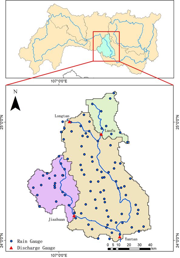
266                                      J. Liu et al.: Ensemble streamflow forecasting over a cascade reservoir catchment

cal processes, capturing the nonlinear characteristics of hy-      well studied, it is challenging to reproduce the reservoir op-
drologic system and parameterizing models (Hornberger and          erating rules in a physical model (Gao et al., 2010; Zhang et
Boyer, 1995; Kirchner, 2006). With advancements in com-            al., 2016; Dang et al., 2020).
puter technology and high-resolution observation, a well-             Machine learning methods can recognize patterns hid-
parameterized hydrological model can now simulate stream-          den in input data and can simulate or predict streamflow
flow with high accuracy (Kollet et al., 2010; Ye et al., 2014;     without explicit descriptions of the underlying physical pro-
Graaf et al., 2015; Yuan et al., 2018b).                           cesses (Kisi, 2007; Adnan et al., 2019). Neural networks are
   Streamflow simulations from hydrological models heavily         suitable for streamflow forecasting among machine learn-
rely on meteorological forcing inputs, especially precipita-       ing models, and some of them can even outperform phys-
tion, which can be measured at in situ gauges or retrieved         ically based hydrological models. For example, Humphrey
from satellites and radars. However, for medium-range (2–          et al. (2016) showed that their combined Bayesian artificial
15 d ahead) streamflow forecasts, precipitation forecasts are      neural network (ANN) with the modèle du Génie Rural à
needed (Hopson and Webster, 2010). To improve the fore-            4 paramètres Journalier (GR4J) approach outperforms the
casts, ensemble techniques that can give a deterministic esti-     GR4J model with respect to monthly streamflow forecasting.
mate as well as the estimate’s uncertainty have become pop-        Kratzert et al. (2019) showed that an approach based on the
ular. Ensemble weather forecasting can be traced back to           long short-term memory (LSTM) technique outperforms a
1963 (Lorenz, 1963). Later, Leith (1974) transferred a de-         well-calibrated Sacramento Soil Moisture Accounting Model
terministic forecast into an ensemble using the Monte Carlo        (SAC-SMA). Yang et al. (2020) used a geomorphology-
method in order to describe the atmospheric uncertainty. In        based hydrological model (GBHM) combined with a tradi-
the 1990s, ensemble forecasting was developed into an inte-        tional ANN model to simulate daily streamflow, which can
gral part of numerical weather prediction that showed higher       provide enough physical evidence and can run with less ob-
skill than the deterministic forecast, even with higher model      servation data. Although neural network models are criti-
resolution (Toth et al., 2001). Due to the rapid development       cized with little physical evidence (Abrahart et al., 2012),
of this technique, ensemble weather forecasting and climate        their potential in hydrological forecasting is yet to be ex-
predictions are applied to hydrological forecasting studies        plored.
by combining them with hydrological models (Jasper et al.,            In this study, we combine machine learning with a hy-
2002; Balint et al., 2006; Jaun et al., 2008; Xu et al., 2015;     drometeorological approach for hourly streamflow forecast-
Yuan et al., 2016; Zhu et al., 2019). Provided with an ensem-      ing over a cascade reservoir catchment located in south-
ble of streamflow forecasts and their forecast variability, a      western China. We use the meteorological hindcast data
reservoir can maintain a reliable utility from natural stream-     from the European Centre for Medium-Range Weather Fore-
flow better than that provided with a deterministic streamflow     casts (ECMWF) model that participated in the THORPEX
forecast only (Zhao et al., 2011). However, the streamflow         (THe Observing-system Research and Predictability EXper-
prediction skill depends on whether the precipitation fore-        iment) Interactive Grand Global Ensemble (TIGGE) project
casts introduced into the hydrological model are skillful (Al-     to drive a newly developed high-resolution land surface
fieri et al., 2013). When assessing the skill of this hydromete-   model, named “CSSPv2” (Conjunctive Surface-Subsurface
orological forecasting approach, a benchmark is needed. Us-        Process, version 2; Yuan et al., 2018b), to provide runoff
ing ensembles of historical climatology data (Day, 1985) as        and streamflow forecasts, and we corrected the forecasts us-
meteorological forecast inputs, which is known as ensemble         ing the LSTM model. We aim to improve flood forecasting
streamflow prediction (ESP), is often selected as the bench-       over the cascade reservoir catchment by integrating meteoro-
mark approach. Evaluations of hydrological forecasts have          logical forecasts, hydrological modeling and machine learn-
indicated that forecast skill has a close relationship with the    ing. So we strive to (1) calibrate the hydrological model,
catchment size, geographical location and resolution (Alfieri      (2) bias correct the meteorological forecasts, (3) evaluate the
et al., 2013; Pappenberger et al., 2015); thus, there is a ne-     streamflow forecast skill and (4) test the combined physical–
cessity to compare these forecasts with the ESP in order to        statistical approach.
establish the skill of the hydrometeorological forecasting ap-
proach.
   Although physically based hydrological models are widely        2     Study area, data, model and method
used, it is still hard to apply a hyper-resolution distributed
model to streamflow forecasting due to its demand for ob-          2.1    Study area
servation data, its complex model structures, and the compu-
tational resource requirements for calibration and application     The Yantan Hydropower Station is in the middle reaches
(Wood et al., 2011; Kratzert et al., 2018; Yaseen et al., 2018).   of the Hongshui River in Dahua Yao Autonomous County,
In cascade reservoir systems, there are two sources of stream-     Guangxi Province. This station is the fifth level in the 10-
flow: the rainfall within the interval basin and the upstream      level development of the Hongshuihe hydropower base in
reservoir discharge. While the rainfall–runoff relationship is     the Nanpanjiang River, connected with the upstream Longtan

Hydrol. Earth Syst. Sci., 26, 265–278, 2022                                            https://doi.org/10.5194/hess-26-265-2022
J. Liu et al.: Ensemble streamflow forecasting over a cascade reservoir catchment                                              267

                                                                   2.2     Data and method

                                                                   2.2.1    Hydrometeorological observations

                                                                   There are 97 meteorological observation stations within the
                                                                   catchment (Fig. 1). Here, observed hourly 2 m temperature,
                                                                   10 m wind speed, relative humidity, accumulated precipita-
                                                                   tion and surface pressure data were interpolated onto a 5 km
                                                                   gridded observation dataset using the inverse distance weight
                                                                   method. The hourly surface downward solar radiation data
                                                                   from the China Meteorological Administration Land Data
                                                                   Assimilation System (CLDAS) were also interpolated onto
                                                                   a 5 km dataset using the bilinear interpolation method. The
                                                                   hourly surface downward thermal radiation was estimated by
                                                                   specific humidity, pressure and temperature. This dataset was
                                                                   used to drive the CSSPv2 land surface hydrological model.
                                                                      The monthly runoff for each 5 km grid was estimated by
                                                                   disaggregating control streamflow station observations with
                                                                   the ratio of observed grid monthly precipitation and catch-
                                                                   ment mean precipitation. The gridded runoff was used to cal-
                                                                   ibrate the CSSPv2 model at each grid (Yuan et al., 2016). The
                                                                   calibrated runoff parameters can be used to better represent
                                                                   the heterogeneity of the rainfall–runoff processes and make
                                                                   precise runoff simulations.

                                                                   2.2.2    Ensemble meteorological hindcast data and ESP
                                                                            hindcasts

Figure 1. Locations of discharge gauges and rain gauges over the   The TIGGE dataset consists of ensemble forecast data from
Yantan Basin.                                                      10 global numerical weather prediction centers starting from
                                                                   October 2006; the dataset has been made available for sci-
Table 1. Information on hydrological gauges.                       entific research via data archive portals at ECMWF and the
                                                                   China Meteorological Administration (CMA). TIGGE has
 Gauge       Longitude   Latitude   Drainage area                  become the focal point for a range of research projects,
               (◦ E)      (◦ N)     (km2 )                         including research on ensemble forecasting, predictability
 Longtan      107.09       25.00    –                              and the development of products to improve the prediction
 Yantan       107.50       24.11    5950 (orange area in Fig. 1)   of severe weather (Bougeault et al., 2010). In this paper,
 Luofu        107.36       24.90    800 (green area in Fig. 1)     TIGGE data from April to September during 2013–2017
 Jiazhuan     107.12       24.21    2150 (purple area in Fig. 1)   from ECMWF were used as meteorological hindcast data.
                                                                   The 3-hourly meteorological hindcasts for a 7 d lead time
                                                                   from 51 ensemble members (including a control forecast)
Hydropower Station and the downstream Dahua Hydropower             were interpolated to a 5 km resolution via bilinear interpo-
Station. The drainage area between the Longtan Hydropower          lation. The forecast precipitation and temperature were cor-
Station and Yantan Hydropower Station is 8900 km2 . The            rected to match the observational means in order to remove
annual mean streamflow at the Yantan hydrological gauge            the biases.
is 55.5 ×10⁹ m3 . The river passes through a karst mountain           The ESP was accomplished by applying historical meteo-
area, with a narrow valley, steep slope and scattered culti-       rological forcings (Day, 1985). In this paper, the meteorolog-
vated land, and the average slope is 0.036 %. Figure 1 shows       ical forcings from the same date as the forecast start date to
the locations of four hydrological gauges, with detailed in-       the next 9 d of each year (excluding the target year) were se-
formation listed in Table 1.                                       lected as the ESP forcings. Take 1 April 2013 as an example,
                                                                   the 7 d observation periods starting from 1 to 10 April (i.e.,
                                                                   1–7 April, 2–8 April, . . . , 10–16 April) in the years 2014,
                                                                   2015, 2016 and 2017 were selected as the forecast ensem-
                                                                   ble forcings of the issue date (1 April), resulting in a total of

https://doi.org/10.5194/hess-26-265-2022                                           Hydrol. Earth Syst. Sci., 26, 265–278, 2022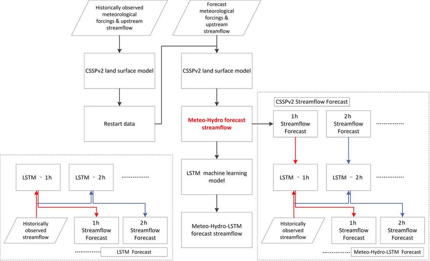
268                                      J. Liu et al.: Ensemble streamflow forecasting over a cascade reservoir catchment

40 ensemble members. The detailed information on the raw
datasets is given in Table 2.
                                                                   W = 1.956 × A0.413
                                                                                acc ,                                         (3)
2.2.3   CSSPv2 streamflow hindcasts
                                                                   H   = 0.245 × A0.342
                                                                                  acc ,                                       (4)
The physical hydrological model used in this paper is the                                      Hmax − H
                                                                   n = 0.03 + (0.05 − 0.03)               ,                   (5)
Conjunctive Surface-Subsurface Process model, version 2                                       Hmax − Hmin
(CSSPv2; Yuan et al., 2018b). The CSSPv2 model is a dis-
tributed, grid-based land surface hydrological model that was      where W , H and n are river width (m), depth (m) and
developed from the Common Land Model (Dai et al., 2003,            roughness (unitless) for each 5 km grid; Aacc is the upstream
2004), but it has better representations of lateral surface and    drainage area (km2 ); and Hmax and Hmin refer to the max-
subsurface hydrological processes and their interactions. The      imum and minimum values of river depth calculated by
routing model used here employs the kinetic wave equation          Eq. (4).
as a covariance function, which is solved via a Newton algo-          Using a trial-and-error procedure, we calibrated these river
rithm. A main reason for adopting this covariance function is      channel parameters to match the simulated streamflow with
that it suits basins with mountainous terrain. The CSSPv2          observed hourly records at the Yantan hydrological gauge.
model was successfully used to perform a high-resolution           The simulation results were evaluated by calculating the
(3 km) land surface simulation over the Sanjiangyuan region,       Nash–Sutcliffe efficiency (NSE) with corresponding obser-
which is the headwater of major Chinese rivers (Ji and Yuan,       vation data. The descriptions of the calibrated parameters and
2018). In this paper, we calibrated the CSSPv2 model against       their ranges are given in Table 3.
monthly estimated runoff to simulate the natural hydrolog-            After calibration, we drove the CSSPv2 model using 5 km
ical processes using the shuffled complex evolution (SCE-          regridded and bias-corrected TIGGE-ECMWF forecast forc-
UA) approach (Duan et al., 1994). The calibrated param-            ing during 2013–2017 to provide a set of 7 d hindcasts.
eters include the maximum velocity of baseflow, the vari-          Streamflow hindcasts from both the ESP and the hydrom-
able infiltration curve parameter, the fraction of maximum         eteorlogical approach (TIGGE-ECMWF/CSSPv2, where
soil moisture where nonlinear baseflow occurs and the frac-        CSSPv2 was driven by TIGGE-ECMWF) were corrected by
tion of maximum velocity of baseflow where nonlinear base-         matching monthly mean streamflow observations to remove
flow begins. The hourly observed streamflow at the Yan-            the biases, and the hindcast experiments were termed “ESP-
tan hydrological gauge was used to manually calibrate the          Hydro” and “Meteo-Hydro” (Table 4). Figure 2 shows the
CSSPv2 routing model, including the slope, river density,          procession of the CSSPv2 hindcasts: the calibrated CSSPv2
roughness, width and depth. The observed streamflow values         model was first driven with the observation dataset to gen-
at the Longtan hydrological gauge were added into the corre-       erate initial hydrological conditions (e.g., soil moisture and
sponding grid to provide upstream streamflow information.          surface water) for each forecast issue date, and the CSSPv2
We used a high-resolution elevation database (hereafter re-        model was then driven with forecast data (TIGGE-ECMWF
ferred to as DEM90) for sub-grid parameterization and then         or ESP) at every forecast issue date with the generated initial
calculated the initial values of these river channel parame-       conditions to perform a 7 d hindcast.
ters. We first extracted the slope angle and the natural river
flow path from DEM90 and then identified the accurate river        2.2.4    LSTM streamflow forecast
network using a drainage area threshold of 0.18 km2 . River
density and bed slope values for each 5 km grid were calcu-        Long short-term memory (LSTM) is a type of recurrent neu-
lated as follows:                                                  ral network model that learns from sequential data. The input
          X                                                        of the LSTM model includes the forecast interval stream-
rivden =       l/A,                                          (1)   flow at the specified forecast step obtained from TIGGE-
                                                                   ECMWF/CSSPv2, historical upstream streamflow observa-
bedslp = mean(tan(β)),                                      (2)
                                                                   tions and historical streamflow observations at the Yantan hy-
where rivden is the river density (km/km2 ), bedslp is the river   drological gauge. The network was trained on sequences of
channelP  bed slope (unitless), A is the area of a 5 km grid       April to September data from 2013 to 2017, with six histori-
(km2 ),    l is the total river channel length (m) within the      cal streamflow observations and one forecast interval stream-
grid and β is the slope angle (radian) for each river segment      flow to predict the total streamflow at each forecast time step
located in the grid.                                               (Fig. 2). The LSTM was calibrated using a cross validation
   Other river channel parameters were estimated using em-         method by leaving the target year out.
pirical formulas (Getirana et al., 2012; Luo et al., 2017) as         Before calibration, all input and output variables were nor-
follows:                                                           malized as follows:
                                                                             (q − qmin )
                                                                   q0 =                   ,                                   (6)
                                                                           (qmax − qmin )

Hydrol. Earth Syst. Sci., 26, 265–278, 2022                                            https://doi.org/10.5194/hess-26-265-2022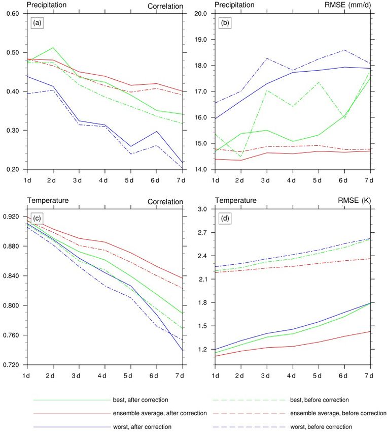
J. Liu et al.: Ensemble streamflow forecasting over a cascade reservoir catchment 269
Table 2. Information on hydrological datasets. (Please note that dates are given in the following format in this table: yyyy/mm/dd.)
Dataset Time range Time step
Rain gauge observation forcing 2013/1/1–2017/12/31 Hourly
Longtan & Yantan discharge gauge streamflow data 2013/1/1–2017/12/31 Hourly
Jiazhuan & Luofu discharge gauge streamflow data 2013/4/1–2017/9/30 Daily
TIGGE-ECMWF forecast forcing 2013/4/1–2017/9/30 Hourly
Table 3. Descriptions of calibrated parameters.
Parameters Range
Maximum velocity of baseflow (mm/d) 0.00000116–0.000579
Fraction of maximum velocity of baseflow where nonlinear 0.001–0.99
baseflow begins
Fraction of maximum soil moisture where nonlinear 0.2–0.99
baseflow occurs
Variable infiltration curve parameter 0.001–1
River width (m) 0–101.16
River depth (m) 0–6.46
River density (km/km2 ) 0.049–1.03
River roughness 0.033–0.05
River slope 0.015–0.47
where q0 , q, qmax and qmin are the normalized variable, the observation, and F (y) is a cumulative probability distribu-
input variable, and the maximum and minimum of the se- tion curve formed by the forecast ensembles. The CRPS has
quence of the variable, respectively. The hindcast experiment a negative orientation (smaller values are better), and it re-
was termed “Meteo-Hydro-LSTM” (Table 2). In addition, wards the concentration of probability around the step func-
we also tried an LSTM streamflow forecasting approach that tion located at the observed value (Wilks et al., 2005). The
only used 6 h historical streamflow data as inputs; this exper- skill score for deterministic forecast was calculated as
iment was termed “LSTM” (Table 2). The process of LSTM RMSE − RMSEref RMSE
is similar to Meteo-Hydro-LSTM but without the forecast in- SSRMSE = = 1− . (9)
0 − RMSEref RMSEref
terval streamflow, which is also shown in Fig. 2.
The skill score for a probabilistic forecast (CRPSS) could be
2.3 Evaluation method calculated similarly to the SSRMSE .
The root-mean-squared error (RMSE) was used to evaluate
the deterministic forecast, i.e., the ensemble means of 51 3 Results
(ECMWF) or 40 (ESP) forecast members. To evaluate prob-
abilistic forecasts, the continuous ranked probability score 3.1 Evaluation of CSSP calibration
(CRPS) was calculated as follows:
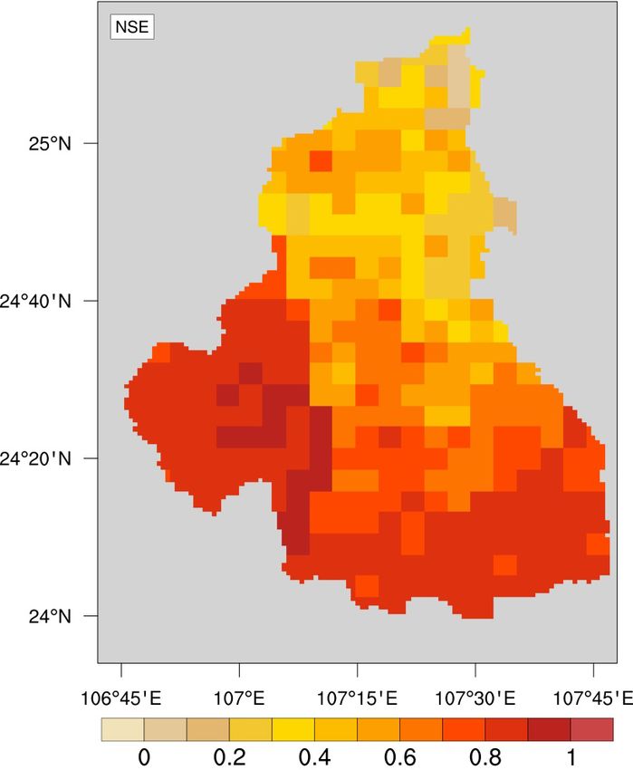
Z ∞ The employed CSSPv2 model is a fully distributed hydrolog-
ical model, and the streamflow is calculated through a pro-
CRPS = [F (y) − Fo (y)]2 , (7)
−∞ cess of converting gridded rainfall into runoff and a process
of runoff routing. Figure 3 shows the runoff calibration re-
where sults by calculating the NSE of monthly runoff simulations
0, y < observed value compared with observed gridded monthly runoff. After cal-
Fo (y) = (8) ibrating the CSSPv2 runoff model, the NSE of all grids are
1, y ≥ observed value
above zero, which indicates that the runoff simulation results
is a cumulative probability step function that jumps from zero in all grids are more reliable than the climatology method.
to one at the point where the forecast variable y equals the In addition, grids distributed in the downstream region have
https://doi.org/10.5194/hess-26-265-2022 Hydrol. Earth Syst. Sci., 26, 265–278, 2022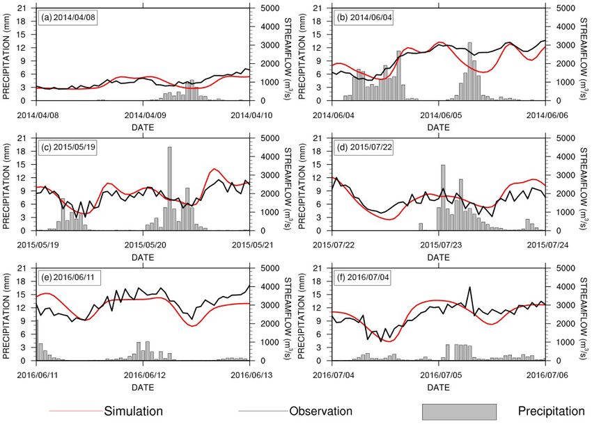
270 J. Liu et al.: Ensemble streamflow forecasting over a cascade reservoir catchment
Table 4. Experimental design in this study.
Experiments Description
ESP-Hydro Using the CSSPv2 land surface hydrological model driven by randomly
sampled historical meteorological forcings
Meteo-Hydro Using the CSSPv2 model driven by bias-corrected TIGGE-ECMWF
hindcast meteorological forcings
Meteo-Hydro-LSTM Using the LSTM model to correct streamflow from the Meteo-Hydro
hindcast
LSTM Using the LSTM model to forecast streamflow based on observations
only
Figure 2. A diagram for the integrated hydrometeorological and machine learning streamflow prediction.
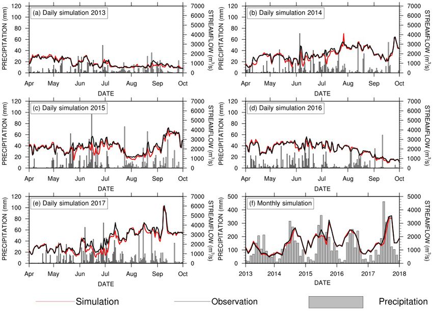
better NSE than the upstream grids. The NSE values of the Figures 4 and 5 show the results after the calibration of
grids in the southern part are greater than 0.5, which ac- the routing model, where CSSPv2 is driven by observed me-
counts for two-thirds of the interval basin area. Higher NSE teorological forcings to provide streamflow simulations and
values in the upstream part of Jiazhuan station (Fig. 1) are compared against observed streamflow at the Yantan hydro-
due to the more humid climate (not shown), as hydrological logical gauge. Figure 4 shows the daily and monthly stream-
models usually have better performance over wetter areas. flow simulation results. The monthly result (Fig. 4f) shows
For the downstream areas with less precipitation, the higher that the simulated streamflow closely follows the observed
NSE values are related to the higher percentage of sand in streamflow, and the NSE is 0.96. The daily streamflow simu-
the soil (not shown). Under the same meteorological condi- lations during flood seasons (Fig. 4a–e) also show good per-
tions, there is higher hydraulic conductivity with higher sand formance, and the NSE is 0.92. During June and July in 2014,
content (Wang et al., 2016), and it yields less runoff under 2015 and 2017, the CSSPv2 model underestimated the daily
infiltration excess, which is more suitable for the saturation- streamflow with a maximum of 1104 m3 /s and an average
excess-based runoff generation for the CSSPv2 model (Yuan of 334 m3 /s (Fig. 4b, c, e). In 2013 and 2016, the difference
et al., 2018b). between the observed and simulated streamflow is relatively
small, and the average difference is 96 m3 /s (Fig. 4a, d).
Hydrol. Earth Syst. Sci., 26, 265–278, 2022 https://doi.org/10.5194/hess-26-265-2022
J. Liu et al.: Ensemble streamflow forecasting over a cascade reservoir catchment                                               271

                                                                      precipitation and temperature (the red dashed lines) than the
                                                                      best ensemble members (the green dashed lines), with an
                                                                      average RMSE reduction of 3.66 mm/d and an average cor-
                                                                      relation increase of 0.04 for precipitation as well as an av-
                                                                      erage RMSE reduction of 0.1 K and an average correlation
                                                                      increase of 0.03 for temperature. After bias correction, the
                                                                      51-ensemble means still perform better than best ensemble
                                                                      members. Compared with the ensemble mean results be-
                                                                      fore bias correction, the RMSE decreased by 0.23 mm/d for
                                                                      the bias-corrected precipitation and decreased by 1 K for the
                                                                      bias-corrected surface air temperature. For the bias-corrected
                                                                      ensemble mean results, the average RMSE and correlation
                                                                      are 14.6 mm/d and 0.44 for precipitation, and they are 1.25 K
                                                                      and 0.87 for surface air temperature.

                                                                      3.3   Comparison between the ESP-Hydro and
                                                                            Meteo-Hydro streamflow forecasts

                                                                      Figure 7 presents the variations in RMSE and CRPS for
                                                                      the ESP-Hydro and Meteo-Hydro hourly streamflow fore-
                                                                      casts at the Yantan hydrological gauge. For the probabilistic
                                                                      forecast, Fig. 7a shows that the CRPS for the Meteo-Hydro
                                                                      streamflow forecast ranges from 165 to 225 m3 /s, while the
                                                                      CRPS for the ESP-Hydro streamflow forecast ranges from
Figure 3. Nash–Sutcliffe efficiency coefficients for the calibrated   170 to 230 m3 /s. The Meteo-Hydro approach performs bet-
grid runoff simulation from CSSPv2.                                   ter than ESP-Hydro, with a lower CRPS at all lead times
                                                                      and an average 6 % improvement in the CRPSS (Fig. 7c).
                                                                      For the deterministic forecast, Fig. 7b shows that the RMSE
   Figure 5 shows the hourly streamflow simulation results            for the Meteo-Hydro streamflow forecast ranges from 250
for a few flood events. Figure 5a shows that the CSSPv2               to 350 m3 /s, while the RMSE for the ESP-Hydro streamflow
model can accurately simulate the streamflow response to a            forecast ranges from 250 to 390 m3 /s. The Meteo-Hydro ap-
rainfall event after a dry period. Figure 5b–d show that the          proach also performs better than ESP-Hydro with a lower
CSSPv2 model overpredicted water loss during the recession            RMSE at all lead times, especially after 3 d, with the average
period for instantaneous heavy rainfall events. Figure 5e–            reduction in the RMSE reaching 6 % (Fig. 7d).
f show that the simulated streamflow has a larger fluctua-               Figure 7 also shows that the forecast skill of both met-
tion than the observations for continuous rainfall events. The        rics have a similar diurnal cycle, where the RMSE and CRPS
simulated streamflow is also smoother than the observations.          reach their peaks at around 00:00 UTC and drop to their lows
Nevertheless, the NSE for the hourly streamflow simulation            at 06:00 UTC. Figure 8 shows the diurnal cycle of the vari-
is 0.61, which suggests that CSSPv2 has acceptable perfor-            ables employed in the model, namely observed catchment
mance on an hourly timescale.                                         mean rainfall and observed streamflow at the Yantan and
                                                                      Longtan hydrological gauges, to explain the diurnal cycle
3.2   Bias correction of the TIGGE-ECMWF                              of the ESP-Hydro and Meteo-Hydro forecasting skill. These
      meteorological forecasts                                        three input variables show different diurnal patterns: the ob-
                                                                      served rainfall starts to rise at 00:00 UTC and reaches its
The resolution of TIGGE-ECMWF grid data is 0.25◦ , so the             maximum at 06:00 UTC; the observed streamflow at the Yan-
data were interpolated onto a 5 km grid to drive the CSSPv2           tan hydrological gauge drops to its minimum at 12:00 UTC
model. We calculated the annual average precipitation and             and rises to its maximum at 00:00 UTC; and the streamflow
temperature for both the observations and TIGGE-ECMWF                 from upstream of the Longtan hydrological gauge starts to
and then performed a bias correction by adding back the               drop at 00:00 UTC and reaches its minimum at 06:00 UTC.
difference (for precipitation) or multiplying back the ratio          After comparing these diurnal cycles with the cycle of fore-
(for temperature) to match the observations’ averages. Fig-           cast skill, it is found that the forecast skill decreases when
ure 6 shows the correlation coefficient and RMSE of TIGGE-            the upstream Longtan outflow starts to decrease and the pre-
ECMWF precipitation and temperature forecasts compared                cipitation starts to increase. When the upstream Longtan out-
against the observations, either before or after bias correc-         flow increases and the precipitation starts to decrease (after
tion. The 51-ensemble mean shows better performance for               06:00 UTC), the forecast skill rises.

https://doi.org/10.5194/hess-26-265-2022                                             Hydrol. Earth Syst. Sci., 26, 265–278, 2022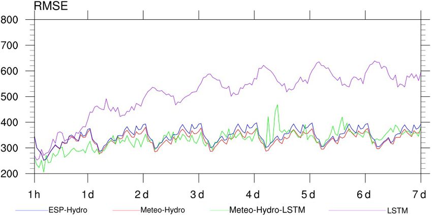
272                                       J. Liu et al.: Ensemble streamflow forecasting over a cascade reservoir catchment

Figure 4. Evaluation of streamflow simulations at the Yantan hydrological gauge. The black and red lines are the observed and simulated
streamflow. Panels (a)–(e) show daily streamflow, and panel (f) shows monthly streamflow. The gray bars represent daily (or monthly)
precipitation.

Figure 5. The same as Fig. 4 but for the evaluation of hourly streamflow simulations at the Yantan hydrological gauge. (Please note that
dates are given in the following format in this figure: yyyy/mm/dd.)

Hydrol. Earth Syst. Sci., 26, 265–278, 2022                                              https://doi.org/10.5194/hess-26-265-2022
J. Liu et al.: Ensemble streamflow forecasting over a cascade reservoir catchment                                                273

Figure 6. Evaluation of precipitation and temperature hindcasts from TIGGE-ECMWF. The red and blue lines represent the best and worst
results among the 51 TIGGE-ECMWF ensemble members, respectively, and the green lines represent the results for the ensemble means of
51 members. Solid and dashed lines represent the results after and before bias corrections, respectively.

3.4   The Meteo-Hydro-LSTM streamflow forecast                       Yantan hydrological gauge as input. Without using the phys-
                                                                     ical model forecast, the RMSE is improved only when the
                                                                     lead time is less than 1 d. Moreover, the performance of
Machine learning methods can recognize patterns hidden in            LSTM is far worse than the Meteo-Hydro streamflow fore-
input data and can simulate or predict streamflow without ex-        cast when the lead time is more than 2 d.
plicit descriptions of the underlying physical processes. Fig-          Figure 10 presents several examples of streamflow fore-
ure 9 shows the RMSE of the Meteo-Hydro-LSTM stream-                 casts using the Meteo-Hydro-LSTM and Meteo-Hydro ap-
flow forecast using the ensemble mean hydrological forecast          proaches to show the forecast improvements in detail. The
as described in the section above and using the past 6 h ob-         Meteo-Hydro-LSTM approach reduced the flood peak value
served streamflow of the Yantan hydrological gauge as input.         and the water loss during flood recession period compared
Compared with the Meteo-Hydro and ESP-Hydro approach,                with the Meteo-Hydro streamflow forecast approach, which
applying the LSTM model can further decrease the RMSE                improves the streamflow prediction for most cases (Fig. 10b–
within the first 72 h. The RMSE of the Meteo-Hydro-LSTM              f). However, when the upstream reservoir’s flood operation
approach ranges from 205 to 363 m3 /s during these 3 days,           is triggered by continuous heavy rain, Meteo-Hydro may un-
suggesting an average 6 % improvement compared with the              derpredict the streamflow. As the LSTM model further de-
Meteo-Hydro approach.                                                creases the streamflow, the Meteo-Hydro-LSTM method can
   Figure 9 also shows the RMSE of the LSTM streamflow               end up worsening the streamflow forecast, which means that
forecast using only the past 6 h observed streamflow of the

https://doi.org/10.5194/hess-26-265-2022                                             Hydrol. Earth Syst. Sci., 26, 265–278, 2022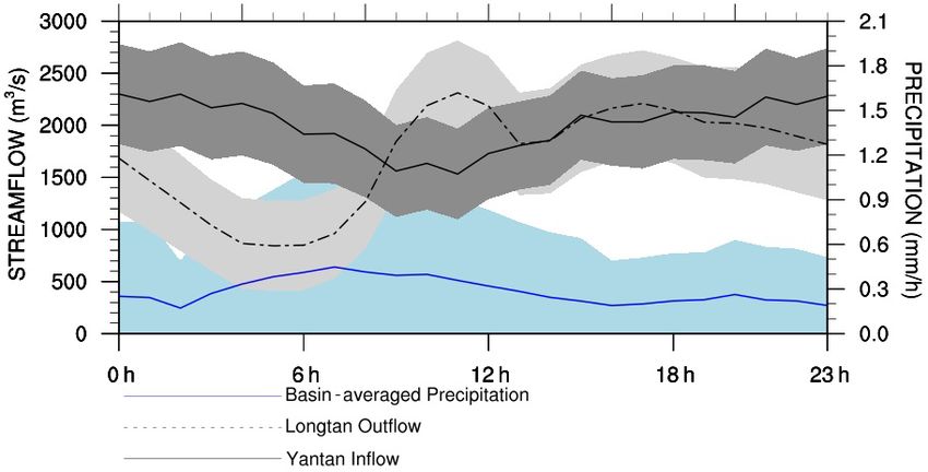
274                                         J. Liu et al.: Ensemble streamflow forecasting over a cascade reservoir catchment

Figure 7. (a) The continuous ranked probability score (CRPS) and (b) root-mean-squared error (RMSE) for the daily streamflow ensemble
forecasts at the Yantan hydrological gauge. Panels (c) and (d) show the skill score in terms of the CRPS and RMSE for Meteo-Hydro, where
ESP-Hydro is used as the reference forecast.

Figure 8. Diurnal cycle of Longtan outflow (m3 /s; dashed black line), Yantan inflow (m3 /s; solid black line) and basin-averaged precipitation
(mm/h; blue line) as well as their ranges. The time shown in this figure is universal time.

the machine learning method may not always improve the                    served streamflow at the Yantan hydrological gauge was used
forecasts (Fig. 10a).                                                     to calibrate the routing module of the CSSPv2 model. The
                                                                          bias-corrected TIGGE-ECMWF ensemble forecasts were
                                                                          then used to drive the CSSPv2 for streamflow forecasts,
4     Conclusions                                                         and the LSTM model was used to correct the stream-
                                                                          flow forecasts, resulting in an integrated meteorological–
In this study, we developed and evaluated a streamflow fore-
                                                                          hydrological–machine learning forecast framework.
casting framework by coupling meteorological forecasts with
                                                                             With automatic offline calibration of the CSSPv2 model,
a land surface hydrological model (CSSPv2) and a machine
                                                                          the NSE values are 0.96, 0.92 and 0.61 for streamflow sim-
learning method (LSTM) over a cascade reservoir catchment
                                                                          ulations at the Yantan hydrological gauge at monthly, daily
using hindcast data from 2013 to 2017. The monthly ob-
                                                                          and hourly timescales, respectively. The bias-corrected en-
served runoff was used to calibrate the runoff generation
                                                                          semble mean TIGGE-ECMWF forcings, which perform the
module of the CSSPv2 model grid by grid, and the hourly ob-

Hydrol. Earth Syst. Sci., 26, 265–278, 2022                                                   https://doi.org/10.5194/hess-26-265-2022
J. Liu et al.: Ensemble streamflow forecasting over a cascade reservoir catchment 275 Figure 9. The RMSE (m3 /s) for the hourly streamflow hindcasts from four forecasting approaches. The green line represents the Meteo- Hydro-LSTM forecast, the red line represents the Meteo-Hydro forecast, the blue line represent the ESP-Hydro forecast and the purple line represents the LSTM forecast based on historical streamflow observations alone. Figure 10. Evaluation of the forecast approaches for a few flooding events. The black lines are observed streamflow from the Yantan hydrological gauge, the blue lines are the Meteo-Hydro ensemble mean streamflow forecast and the red lines are the Meteo-Hydro-LSTM forecast streamflow using the Meteo-Hydro ensemble mean forecast with LSTM. The gray bars represent hourly precipitation averaged over the basin. (Please note that dates are given in the following format in this figure: mm/dd.) best among all ensemble members, show average respective Adding the LSTM model to the hydrometeorological fore- RMSE and correlation values of 14.6 mm/d and 0.44 for pre- cast (Meteo-Hydro-LSTM) can further reduce the forecast cipitation forecasts and 1.3 K and 0.87 for surface air temper- error. Within the first 72 h, LSTM can improve the forecast ature forecasts. By comparing these results with the hourly skill by a maximum of 25 % and an average of 6 %. However, observed streamflow, it is found that the integrated hydrom- if we do not use the streamflow predicted by Meteo-Hydro, eteorological forecast approach (Meteo-Hydro) increases the the error from the LSTM increases rapidly after 24 h, and probabilistic and deterministic forecast skill against the ini- the historical-data-based LSTM method performs worse than tial condition-based approach (ESP-Hydro) by 6 %. the Meteo-Hydro method. Most cascade reservoirs cannot https://doi.org/10.5194/hess-26-265-2022 Hydrol. Earth Syst. Sci., 26, 265–278, 2022
276                                         J. Liu et al.: Ensemble streamflow forecasting over a cascade reservoir catchment

currently forecast streamflow beyond 6 h, and the integrated              chy? Emerging themes and outstanding challenges for neural
Meteo-Hydro-LSTM approach has the potential to improve                    network river forecasting, Prog. Phys. Geogr., 36, 480–513,
the forecasts at long lead times. This study mainly focused on            https://doi.org/10.1177/0309133312444943, 2012.
exploring the added value of meteorology–hydrology cou-                 Adnan, R. M., Liang, Z., Trajkovic, S., Zounemat-Kermani, M.,
pled forecast and LSTM forecasts in a non-closed catch-                   Li, B., and Kisi, O.: Daily streamflow prediction using opti-
                                                                          mally pruned extreme learning machine, J. Hydrol., 577, 123981,
ment; therefore, the forecast uncertainty from upstream out-
                                                                          https://doi.org/10.1016/j.jhydrol.2019.123981, 2019.
flow was ignored by using the observed outflow. In the fu-              Alfieri, L., Burek, P., Dutra, E., Krzeminski, B., Muraro, D., Thie-
ture, it is planned to include the upstream outflow forecast;             len, J., and Pappenberger, F.: GloFAS – global ensemble stream-
however, this will be very challenging, as it requires the de-            flow forecasting and flood early warning, Hydrol. Earth Syst.
velopment of an upstream hydrometeorological forecast ca-                 Sci., 17, 1161–1175, https://doi.org/10.5194/hess-17-1161-2013,
pability as well as reservoir regulation forecasts. Artificial            2013.
intelligence (AI) techniques are expected to complement the             Balint, G., Csik, A., Bartha, P., Gauzer, B., and Bonta, I.: Appli-
physical model for reservoir regulation forecasts.                        cation of meterological ensembles for Danube flood forecasting
                                                                          and warning, in: Transboundary Floods: Reducing Risks through
                                                                          Flood Management, edited by: Marsalek, J., Stancalie, G., and
Data availability. The TIGGE-ECMWF hindcast data can be                   Balint, G., NATO Science Series, Springer, Dordecht, the Nether-
downloaded      from     https://apps.ecmwf.int/datasets/data/tigge/      lands, 57–68, https://doi.org/10.1007/1-4020-4902-1_6, 2006.
levtype=sfc/type=pf/ (Parsons et al., 2017). The in situ observations   Bougeault, P., Toth, Z., Bishop, C., Brown, B., Burridge, D.,
and simulation data are available from the authors upon request.          Chen, D. H., Ebert, B., Fuentes, M., Hamill, T. M., Mylne,
                                                                          K., Nicolau, J., Paccagnella, T., Park, Y., Parsons, D., Raoult,
                                                                          B., Schuster, D., Dias, P. S., Swinbank, R., Takeuchi, Y., Ten-
                                                                          nant, W., Wilson, L., and WorLey, S.: The THORPEX interactive
Author contributions. XY conceived and designed the study. JL
                                                                          grand global ensemble, B. Am. Meteorol. Soc., 91, 1059–1072,
performed the analyses and wrote the initial draft of the paper. XY
                                                                          https://doi.org/10.1175/2010BAMS2853.1, 2010.
revised the paper with substantial contributions from all authors. JZ
                                                                        Dai, Y., Zeng, X., Dickinson, R. E., Baker, I., Bonan, G. B.,
and YJ provided JL with modeling technical support. YL and LZ
                                                                          Bosilovich, M. G., Denning, A. S., Dirmeyer, P. A.,Houser, P.
provided the observed meteorology data used in this study. LY pro-
                                                                          R., Niu, G., Oleson, K. W., Schlosser, C. A., and Yang, Z.: The
vided the observed hydrology data used in this study.
                                                                          Common Land Model, B. Am. Meteorol. Soc., 84, 1013–1024,
                                                                          https://doi.org/10.1175/BAMS-84-8-1013, 2003.
                                                                        Dai, Y., Dickinson, R. E., and Wang, Y. P.: A two-big-leaf model
Competing interests. The contact author has declared that neither         for canopy temperature, photosynthesis, and stomatal conduc-
they nor their co-authors have any competing interests.                   tance, J. Climate, 17, 2281–2299, https://doi.org/10.1175/1520-
                                                                          0442(2004)0172.0.CO;2, 2004.
                                                                        Dang, T. D., Chowdhury, A. F. M. K., and Galelli, S.: On the repre-
Disclaimer. Publisher’s note: Copernicus Publications remains             sentation of water reservoir storage and operations in large-scale
neutral with regard to jurisdictional claims in published maps and        hydrological models: implications on model parameterization
institutional affiliations.                                               and climate change impact assessments, Hydrol. Earth Syst. Sci.,
                                                                          24, 397–416, https://doi.org/10.5194/hess-24-397-2020, 2020.
                                                                        Day, G. N.: Extended Streamflow Forecasting Using NWSRFS, J.
Acknowledgements. We would like to thank the reviewers for their          Water Resour. Plan Manag., 111, 157–170, 1985.
constructive comments and suggestions.                                  de Graaf, I. E. M., Sutanudjaja, E. H., van Beek, L. P.
                                                                          H., and Bierkens, M. F. P.: A high-resolution global-scale
                                                                          groundwater model, Hydrol. Earth Syst. Sci., 19, 823–837,
Financial support. This research has been supported by the Na-            https://doi.org/10.5194/hess-19-823-2015, 2015.
tional Key R&D Program of China (grant no. 2018YFA0606002)              Duan, Q., Sorooshian, S., and Gupta, V. K.: Optimal use of
and the National Natural Science Foundation of China (grant nos.          SCEUA global optimization method for calibrating watershed
41875105 and 41901035).                                                   models, J. Hydrol., 158, 265–284, https://doi.org/10.1016/0022-
                                                                          1694(94)90057-4, 1994.
                                                                        Gao, X., Zeng, Y., Wang, J., and Liu, H.: Immediate im-
Review statement. This paper was edited by Bob Su and reviewed            pacts of the second impoundment on fish communities in the
by Tongtiegang Zhao and three anonymous referees.                         Three Gorges Reservoir, Environ. Biol. Fish., 87, 163–173,
                                                                          https://doi.org/10.1007/s10641-009-9577-1, 2010.
                                                                        Getirana, A. C. V., Boone, A., Yamazaki, D., Decharme, B., Papa,
                                                                          F., and Mognard, N.: The Hydrological Modeling and Anal-
References                                                                ysis Platform (HyMAP): Evaluation in the Amazon Basin, J.
                                                                          Hydrometeorol., 13, 1641–1665, https://doi.org/10.1175/JHM-
Abrahart, R. J., Anctil, F., Coulibaly, P., Dawson, C. W.,                D-12-021.1, 2012.
  Mount, N. J., See, L. M., Shamseldin, A. Y., Solomatine,
  D. P., Toth, E., and Wilby., R. L.,: Two decades of anar-

Hydrol. Earth Syst. Sci., 26, 265–278, 2022                                                https://doi.org/10.5194/hess-26-265-2022
J. Liu et al.: Ensemble streamflow forecasting over a cascade reservoir catchment 277
Hao, Z., Aghakouchak, A., and Phillips, T. J.: Changes in con- Lorenz, E. N.: Deterministic Nonperiodic Flow, J. At-
current monthly precipitation and temperature extremes, En- mos. Sci., 20, 130–141, https://doi.org/10.1175/1520-
viron. Res. Lett., 8, 1402–1416, https://doi.org/10.1088/1748- 0469(1963)0202.0.CO;2, 1963.
9326/8/3/034014, 2013. Luo, X., Li, H.-Y., Leung, L. R., Tesfa, T. K., Getirana, A., Papa,
Hopson, T. and Webster, P.: A 1–10 day ensemble forecasting F., and Hess, L. L.: Modeling surface water dynamics in the
scheme for the major river basins of Bangladesh: forecasting Amazon Basin using MOSART-Inundation v1.0: impacts of geo-
severe floods of 2003–2007, J. Hydrometeorol., 11, 618–641, morphological parameters and river flow representation, Geosci.
https://doi.org/10.1175/2009JHM1006.1, 2010. Model Dev., 10, 1233–1259, https://doi.org/10.5194/gmd-10-
Hornberger, G. M., and Boyer, E. W.: Recent advances 1233-2017, 2017.
in watershed modeling, Rev. Geophys., 33, 949–957, Mulvaney, T.J.: On the use of self-registering rain and flood gauges
https://doi.org/10.1029/95RG00288, 1995. in making observations of the relations of rainfall and flood dis-
Humphrey, G. B., Gibbs, M. S., Dandy, G. C., and Maier, charges in a given catchment, Trans. Inst. Civil Eng. Ireland, 4,
H. R.: A hybrid approach to monthly streamflow fore- 18–33, 1851.
casting: Integrating hydrological model outputs into a Pappenberger, F., Ramos, M. H., Cloke, H. L., Wetterhall, F.,
Bayesian artificial neural network, J. Hydrol., 540, 623–640, Alfieri, L., Bogner, K., Mueller, A., Salamon, P.: How do I
https://doi.org/10.1016/j.jhydrol.2016.06.026, 2016. know if my forecasts are better? Using benchmarks in hy-
Jasper, K., Gurtz, J., and Lang, H.: Advanced flood forecasting in drological ensemble prediction, J. Hydrol., 522, 697–713, 65
Alpine watersheds by coupling meteorological observations and https://doi.org/10.1016/j.jhydrol.2015.01.024, 2015.
forecasts with a distributed hydrological model, J. Hydrol., 267, Parsons, D. B., Beland, M., Burridge, D., Bougeault, P., Brunet, G.,
40–52, https://doi.org/10.1016/S0022-1694(02)00138-5, 2002. Caughey, J., Cavallo, S. M., Charron, M., Davies, H. C., Ni-
Jaun, S., Ahrens, B., Walser, A., Ewen, T., and Schär, C.: A ang, A. D., Ducrocq, V., Gauthier, P., Hamill, T. M., Harr, P.
probabilistic view on the August 2005 floods in the upper A., Jones, S. C., Langland, R. H., Majumdar, S. J., Mills, B.
Rhine catchment, Nat. Hazards Earth Syst. Sci., 8, 281–291, N., Moncrieff, M., Nakazawa, T., Paccagnella, T., Rabier, F.,
https://doi.org/10.5194/nhess-8-281-2008, 2008. Redelsperger, J.-L., Riedel, C., Saunders, R. W., Shapiro, M.
Ji, P., and Yuan, X.: High-resolution land surface modeling A., Swinbank, R., Szunyogh, I., Thorncroft, C., Thorpe, A. J.,
of hydrological changes over the Sanjiangyuan region in Wang, X., Waliser, D., Wernli, H., and Toth, Z.: Thorpex research
the eastern Tibetan Plateau: 2. Impact of climate and land and the science of prediction, B. Am. Meteorol. Soc., 98, 807–
cover change, J. Adv. Model. Earth Syst., 10, 2829–2843, 830, https://doi.org/10.1175/BAMS-D-14-00025.1, 2017 (data
https://doi.org/10.1029/2018MS001413, 2018. available at: https://apps.ecmwf.int/datasets/data/tigge/levtype=
Ji, P., Yuan, X., Jiao, Y., Wang, C., Han, S., and Shi, C.: Anthro- sfc/type=pf/, last access: 12 January 2022).
pogenic contributions to the 2018 extreme flooding over the up- Robertson, D. E. and Wang, Q. J.: Seasonal Forecasts of Un-
per Yellow River basin in China, B. Am. Meteorol. Soc., 101, regulated Inflows into the Murray River, Australia, Water. Re-
S89–S94, https://doi.org/10.1175/BAMS-D-19-0105.1, 2020. sour. Manag., 27, 2747–2769, https://doi.org/10.1007/s11269-
Kirchner, J. W.: Getting the right answers for the right rea- 013-0313-4, 2013.
sons: Linking measurements, analyses, and models to advance Shao, J., Wang, J., Lv, S., and Bing, J.: Spatial and temporal
the science of hydrology, Water Resour. Res., 42, W03S04, variability of seasonal precipitation in Poyang Lake basin and
https://doi.org/10.1029/2005WR004362, 2006. possible links with climate indices, Hydrol. Res., 47, 51–68,
Kisi, O.: Streamflow forecasting using different artificial neu- https://doi.org/10.2166/nh.2016.249, 2016.
ral network algorithms, J. Hydrol. Eng., 12, 532–539, Toth, Z., Zhu, Y., and Marchok, T.: The use of ensem-
https://doi.org/10.1061/(ASCE)1084-0699(2007)12:5(532), bles to identify forecasts with small and large uncertainty,
2007. Weather Forecast, 16, 463–477, https://doi.org/10.1175/1520-
Kollet, S. J., Maxwell, R. M., Woodward, C. S., Smith, S., Vander- 0434(2001)0162.0.CO;2, 2001.
borght, J., Vereecken, H., and Simmer, C.: Proof of concept of re- Wang, R., Zhang, J., Guo, E., Zhao, C., and Cao, T.: Spa-
gional scale hydrologic simulations at hydrologic resolution uti- tial and temporal variations of precipitation concentration
lizing massively parallel computer resources, Water Resour. Res., and their relationships with large-scale atmospheric circu-
46, W04201, https://doi.org/10.1029/2009WR008730, 2010. lations across Northeast China, Atmos. Res., 222, 62–73,
Kratzert, F., Klotz, D., Brenner, C., Schulz, K., and Herrnegger, https://doi.org/10.1016/j.atmosres.2019.02.008, 2019.
M.: Rainfall–runoff modelling using Long Short-Term Mem- Wang, Y., Fan, J., Cao, L., and Liang, Y.: Infiltration and
ory (LSTM) networks, Hydrol. Earth Syst. Sci., 22, 6005–6022, Runoff Generation Under Various Cropping Patterns in the
https://doi.org/10.5194/hess-22-6005-2018, 2018. Red Soil Region of China, Land. Degrad. Dev., 27, 83–91,
Kratzert, F., Klotz, D., Herrnegger, M., Sampson, A. K., https://doi.org/10.1002/ldr.2460, 2016.
Hochreiter, S., and Nearing, G. S.: Toward improved pre- Wei, L., Hu, K.-H., and Hu, X.-D.: Rainfall occurrence and its rela-
dictions in ungauged basins: Exploiting the power of tion to flood damage in china from 2000 to 2015, J. Mt. Sci., 15,
machine learning, Water Resour. Res., 55, 11344–11354, 2492–2504, https://doi.org/10.1007/s11629-018-4931-4, 2018.
https://doi.org/10.1029/2019WR026065, 2019. Wilks, D. S., Dmowska, R., Hartmann, D., and Rossby, T. H.: Sta-
Leith, C. E.: Theoretical Skill of Monte Carlo Forecasts, tistical Methods in the Atmospheric Sciences, second edn., Inter-
Mon. Weather Rev., 102, 409–418, https://doi.org/10.1175/1520- national Geophysics Series, volume 91, Academic Press, ISBN
0493(1974)1022.0.CO;2, 1974. 9780080456225, 2005.
https://doi.org/10.5194/hess-26-265-2022 Hydrol. Earth Syst. Sci., 26, 265–278, 2022278 J. Liu et al.: Ensemble streamflow forecasting over a cascade reservoir catchment Wood, E. F., Roundy, J. K., Troy, T. J., van Beek, L. P. H., Bierkens, Yuan, X., Ma, F., Wang, L., Zheng, Z., Ma, Z., Ye, A., and Peng, S.: M. F. P., Blyth, E., de Roo, A., Döll, P., Ek, M., Famiglietti, An experimental seasonal hydrological forecasting system over J., Gochis, D., van de Giesen, N., Houser, P., Jaffé, P. R., Kol- the Yellow River basin – Part 1: Understanding the role of ini- let, S., Lehner, B., Lettenmaier, D. P., Peters-Lidard, C., Siva- tial hydrological conditions, Hydrol. Earth Syst. Sci., 20, 2437– palan, M., Sheffield, J., Wade, A., and Whitehead, P.: Hyperres- 2451, https://doi.org/10.5194/hess-20-2437-2016, 2016. olution global land surface modeling: Meeting a grand challenge Yuan, X., Wang, S., and Hu, Z.-Z.: Do climate change and El Niño for monitoring Earth’s terrestrial water, Water Resour. Res., 47, increase likelihood of Yangtze River extreme rainfall?, B. Am. W05301, https://doi.org/10.1029/2010WR010090, 2011. Meteorol. Soc., 99, S113–S117, https://doi.org/10.1175/BAMS- Xu, Y. P., Gao, X., Zhu, Q., and Zhang, Y.: Coupling D-17-0089.1, 2018a. a regional climate model and distributed hydrological Yuan, X., Ji, P., Wang, L., Liang, X. Z., Yang, K., Ye, A., model to assess future water resources in Jinhua River Su, Z., and Wen, J.: High-resolution land surface mod- Basin, East China, ASCE J. Hydrol. Eng., 20, 04014054, eling of hydrological changes over the Sanjiangyuan re- https://doi.org/10.1061/(ASCE)HE.1943-5584.0001007, 2015. gion in the eastern Tibetan plateau: 1. Model development Yang, S., Yang, D., Chen, J., Santisirisomboon, J., and Zhao, B.: and evaluation, J. Adv. Model Earth Syst., 10, 2806–2828, A physical process and machine learning combined hydrolog- https://doi.org/10.1029/2018MS001412, 2018b. ical model for daily streamflow simulations of large water- Zhang, Y., Erkyihum, S. T., and Block, P.: Filling the GERD: sheds with limited observation data, J. Hydrol., 590, 125206, evaluating hydroclimatic variability and impoundment strate- https://doi.org/10.1016/j.jhydrol.2020.125206, 2020. gies for Blue Nile riparian countries, Water Int., 41, 593–610, Yaseen, Z. M., Sulaiman, S. O., Deo, R. C., and Chau, K.-W.: An https://doi.org/10.1080/02508060.2016.1178467, 2016. enhanced extreme learning machine model for river flow fore- Zhao, T. T. G., Cai, X. M., and Yang, D. W.: Effect casting: State-of-the-art, practical applications in water resource of streamflow forecast uncertainty on real-time reser- engineering area and future research direction, J. Hydrol., 569, voir operation, Adv. Water Resour., 34, 495–504, 387–408, https://doi.org/10.1016/j.jhydrol.2018.11.069, 2018. https://doi.org/10.1016/j.advwatres.2011.01.004, 2011. Ye, A., Duan, Q., Yuan, X., Wood, E. F., and Zhu, E., Yuan, X., and Wood, A.: Benchmark Decadal Forecast Skill Schaake, J.: Hydrologic post-processing of MOPEX for Terrestrial Water Storage Estimated by an Elasticity Frame- streamflow simulations, J. Hydrol., 508, 147–156, work, Nat. Commun., 10, 1237, https://doi.org/10.1038/s41467- https://doi.org/10.1016/j.jhydrol.2013.10.055, 2014. 019-09245-3, 2019. Hydrol. Earth Syst. Sci., 26, 265–278, 2022 https://doi.org/10.5194/hess-26-265-2022
You can also read