Dynamic risk-based optimization on cryptocurrencies
←
→
Page content transcription
If your browser does not render page correctly, please read the page content below
The current issue and full text archive of this journal is available on Emerald Insight at:
                        https://www.emerald.com/insight/2514-4774.htm

  Dynamic risk-based optimization                                                                                         Risk-based
                                                                                                                      optimization on
       on cryptocurrencies                                                                                            cryptocurrencies
                                     Bayu Adi Nugroho
              Sekolah Tinggi Ilmu Ekonomi YKPN, Yogyakarta, Indonesia

Abstract
                                                                                                                        Received 13 January 2021
Purpose – It is crucial to find a better portfolio optimization strategy, considering the cryptocurrencies’ Revised 17 February 2021
asymmetric volatilities. Hence, this research aimed to present dynamic optimization on minimum variance Accepted 25 February 2021
(MVP), equal risk contribution (ERC) and most diversified portfolio (MDP).
Design/methodology/approach – This study applied dynamic covariances from multivariate GARCH(1,1)
with Student’s-t-distribution. This research also constructed static optimization from the conventional MVP,
ERC and MDP as comparison. Moreover, the optimization involved transaction cost and out-of-sample analysis
from the rolling windows method. The sample consisted of ten significant cryptocurrencies.
Findings – Dynamic optimization enhanced risk-adjusted return. Moreover, dynamic MDP and ERC could
win the naı€ve strategy (1/N) under various estimation windows, and forecast lengths when the transaction cost
ranging from 10 bps to 50 bps. The researcher also used another researcher’s sample as a robustness test.
Findings showed that dynamic optimization (MDP and ERC) outperformed the benchmark.
Practical implications – Sophisticated investors may use the dynamic ERC and MDP to optimize
cryptocurrencies portfolio.
Originality/value – To the best of the author’s knowledge, this is the first paper that studies the dynamic
optimization on MVP, ERC and MDP using DCC and ADCC-GARCH with multivariate-t-distribution and
rolling windows method.
Keywords Cryptocurrencies, Minimum variance, Equal risk contribution, Most diversified portfolio,
Multivariate GARCH
Paper type Research paper

1. Introduction
The popularity of cryptocurrencies has attracted investors to add cryptocurrencies into their
portfolios. The purpose of adding cryptocurrencies is to gain a diversification advantage
(Kajtazi and Moro, 2019; Urquhart and Zhang, 2019; Bouri et al., 2020). However, the increasing
risk of cryptocurrencies has raised some concerns (Palamalai et al., 2020). Moreover,
cryptocurrencies tend to have asymmetric volatility (Baur and Dimpfl, 2018). Therefore, finding
portfolio optimization techniques that result in minimal estimation errors is challenging.
   Several studies investigated the performance of cryptocurrencies portfolio under different
optimization techniques (Platanakis et al., 2018; Symitsi and Chalvatzis, 2018; Brauneis and
Mestel, 2019; Guesmi et al., 2019; Kajtazi and Moro, 2019; Liu, 2019; Platanakis and Urquhart,
2019; Schellinger, 2020; Susilo et al., 2020). However, Markowitz’s approach (Markowitz, 1952)
has two noticeable drawbacks based on theoretical perspectives (Kaucic et al., 2019).
First, Markowitz’s approach precipitately disregards variables with negatively skewed
distribution. Second, investors are more anxious concerning downside risk.
   Risk-based strategies can minimize Markowitz’s drawbacks. Some of the most popular
approaches are equal risk Contribution (ERC), minimum variance (MVP) and most diversified

JEL Classification — F30, G11, G15
    © Bayu Adi Nugroho. Published in Journal of Capital Markets Studies. Published by Emerald
Publishing Limited. This article is published under the Creative Commons Attribution (CC BY 4.0) license.
Anyone may reproduce, distribute, translate and create derivative works of this article (for both
commercial and non-commercial purposes), subject to full attribution to the original publication and                  Journal of Capital Markets Studies
authors. The full terms of this license may be seen at http://creativecommons.org/licences/by/4.0/                          Emerald Publishing Limited
                                                                                                                                              2514-4774
legalcode                                                                                                               DOI 10.1108/JCMS-01-2021-0002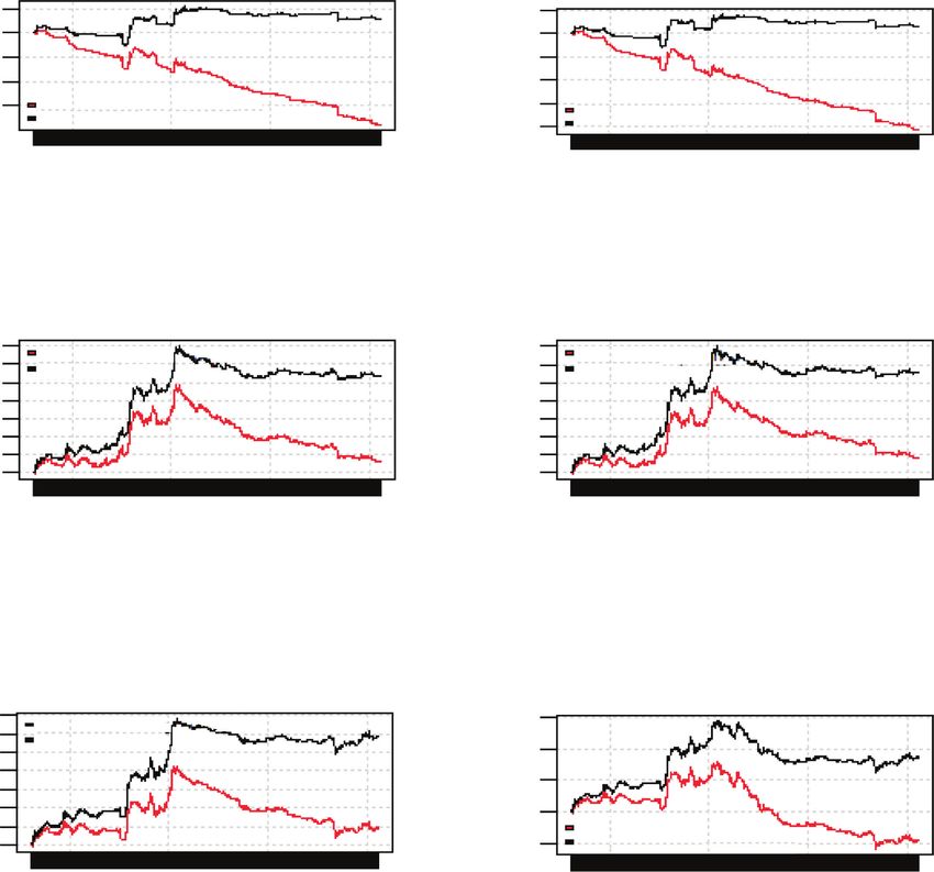
JCMS   portfolio (MDP). Choueifaty and Coignard (2008) implied that holding assets that are not
       perfectly correlated could lead to diversification. Further, MDP was exceptionally well
       regarding relative performance (Choueifaty et al., 2013). Also, ERC defines that a weight vector
       can attain diversification. The weight is obtained from a diversified portfolio concerning its
       constituents’ risk allocations (Qian, 2006, 2011). Notably, there is one similarity in the original
       ERC and MDP: the approaches do not use time-varying covariances or correlations. Therefore,
       this study uses dynamic parameters from GARCH estimations to create a dynamic portfolio.
          The present study attempted to answer the following question: Do risk-based portfolios
       using multivariate GARCH enhance portfolio performance compared with the conventional
       approaches and the naı€ve approach (1/N)? Hence, this research applied dynamic optimization
       on MVP, ERC and MDP. Moreover, this study used dynamic covariances from multivariate
       GARCH with the Student’s t-distribution. Also, this research applied the method of rolling
       windows with various GARH refits.
          Further, this study varies in many respects from previous literature. Some research
       explored the diversification advantage through multivariate GARCH based on bivariate
       portfolios (Basher and Sadorsky, 2016; Ahmad et al., 2018; Jalkh et al., 2020; Yousaf and Ali,
       2020a, 2020b), while this study applies GARCH estimations on ten risky assets. Second,
       previous studies extensively used dynamic hedge ratios and optimal weights strategy (Pal
       and Mitra, 2019; Antonakakis et al., 2020; Bouri et al., 2020; Yousaf and Ali, 2020b). This study
       implements three risk-based approaches. Third, while the conventional ERC, MVP and MDP
       optimization do not use time-varying covariances, this study applies dynamic parameters
       from multivariate GARCH. Fourth, this study uses multivariate Student’s t to account for
       skewed distribution (Antonakakis et al., 2020). Fifth, this study captures extreme volatilities
       into account in the period of COVID-19 pandemic and the years 2017 and 2018. Thus, this
       research mimics real investment. Kajtazi and Moro (2019) opted to disregard the extreme
       volatilities.
          There are two consequences, one investor-oriented and one that activates future study.
       For investment managers, the importance of finding models that can minimize estimation
       error in portfolio optimization is significant. Put differently, improving estimation error in
       covariances can enhance portfolio diversification gains, which is hugely significant,
       considering the crypto market’s stylized facts. The findings of this research can improve
       investors’ understanding of concerning crypto market.
          The second implication is that this research paves the way for future research-other risk-
       based methods, such as inverse volatility, efficient risk portfolio and maximum-decorrelation.
       Moreover, the application of other GARCH specifications such as Copula GARCH is left for
       future research.
          This paper is structured as follows. Section 2 shows the method and data used in this
       study. Section 3 discusses the findings. Section 4 exhibits a robustness check. The last part is
       the conclusion.

       2. Methodology
       This research applied risk-based strategies. Portfolio construction was referring to static and
       dynamic optimization. The covariances used in static optimization were not time-varying,
       while dynamic optimization implemented time-varying covariances from GARCH modeling.
       The covariance of multivariate GARCH was obtained from the rolling windows method to
       create an out-of-sample analysis (Basher and Sadorsky, 2016; Ahmad et al., 2018). Moreover,
       the researcher conducted all calculations in “R” data analysis software, and some of the
       packages used in this research were RiskPortfolios (Ardia et al., 2017b), rmgarch (Ghalanos,
       2019), FRAPO (Pfaff, 2016) and fPortfolio (Wuertz et al., 2017). This study also only had one
       portfolio constraint, which was long-only, to provide a detailed comparison between static
       and dynamic optimization.
2.1 Data                                                                                                  Risk-based
This paper is exploratory research. In line with previous studies, this research used the             optimization on
majority of the sample from other researchers (Antonakakis et al., 2019; Liu, 2019). This
research used ten major cryptocurrencies in portfolio construction. The cryptos were Bitcoin
                                                                                                      cryptocurrencies
(BTC), Ethereum (ETH), Ripple (XRP), Litecoin (LTC), Stellar (XLM), Monero (XMR), Dash
(DASH), Tether (USDT), Nem (XEM) and Dogecoin (DOGE). The researcher obtained daily
prices of the cryptocurrencies (CC) from www.coinmarketcap.com. Following previous
literature (Liu, 2019; Schellinger, 2020), this research took into account the cryptocurrency
bubbles from mid-2017 until the beginning of 2018. This approach reflects a realistic portrait
of the cryptos, and it gives a more informed investment strategy. Furthermore, the sample
period was started from August 8, 2015, to October 20, 2020, indicating 1900 observations.

2.2 Risk-based portfolios
This paper applied risk-based strategies (Ardia et al., 2017a): MV, MDP and ERC portfolio.
Besides, this research also created the hard-to-beat naı€ve strategy (EWP) or 1/N (DeMiguel
et al., 2007).
    MVP strategy:
                                                  N X
                                                  X N
                              minimize → σ 2p ¼                    σ a;b wa wb                  (1)
                                                   j¼1       j¼1

where σ 2p is the variance of p portfolio, and σ i;j is the covariance of asset aP
                                                                                 and asset b.
   MDP is referring to Choueifaty and Coignard’s (2008) findings. If               represents the
variance of the covariance matrix of N assets, the diversification ratio (DR) for a weight vector
ω in a portfolio Ω is defined as
                                                         0
                                                     ωσ
                                       DRω∈Ω ¼ pffiffiffiffiffiffiffiffiffiffiffiffiffi
                                                     P                                          (2)
                                                   0
                                                     ω ω

The denominator is portfolio standard deviation, while the numerator is the weighted
average of asset volatility. The decomposition of Eqn 2 is
                                                   1
                                 DRω∈Ω ¼ pffiffiffiffiffiffiffiffi                                (3)
                                             ðδþCRÞ  δCR

where δ is the volatility-weighted average correlation and CR is the volatility-weighted
concentration ratio. Highly correlated assets are poorly diversified. Choueifaty et al. (2013)
then showed the following formula for MDP strategy

                                               arg max DR
                                      PMDP ¼                                                    (4)
                                                   ωeΩ
              0
Minimizing ω C ω leads to maximum DR, where C is the correlation matrix. This treatment is
similar to MV optimization, but rather than using a covariance matrix, MDP uses a
correlation matrix.
    (ERC is characterized by a minimum asset allocation concerning the risk contribution to
its portfolio (Qian, 2006, 2011; Maillard et al., 2010). The definition of risk contribution is
                                                     vMω∈Ω
                                     Ca Mω∈Ω ¼ ωa                                               (5)
                                                       vωa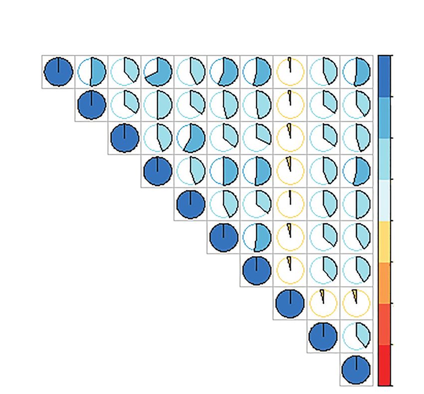
JCMS                    where ωa is the weight of a asset and Mω∈Ω is the portfolio’s standard deviation. Hence, the
                        optimization problem of ERC is
                                                           X             X
                                                  PERC: ωa      ω ¼ ωb             ω ∀a; b;
                                                                    a                  b                         (6)
                                                        0 ≤ ωa ≤ 1 for a ¼ 1; . . . ; N ;
                                                                    0
                                                                  ωa¼1
                        where a is a vector ðN 3 1Þ of 1s. The optimization’s goal is to minimize the risk contributions.
                        Assets with high volatilities get low weights.
                           While the previous study used around 360 days of estimation windows for covariance
                        creation (Liu, 2019; Schellinger, 2020), this study used different optimization days (see
                        Figures 1 and 2).
                           Further, the covariance in the static approach is as follows:
                                                                        1 X  M
                                             σ a;b ¼ Covða; bÞ ¼                ðrat  r a Þ$ðrbt  r b Þ; a; b ¼ 1; . . . ; N                              (7)
                                                                      M  1 t¼1

                        where r a is the mean returns of asset a of N assets in M periods. The variance is when a 5 b.
                        Eqn 7 is called the sample variance-covariance matrix.

                                             Optimization Days VS Sortino Ratio                                Optimization Days VS Sortino Ratio
                                             No Transaction Cost-Static Approach                               With Transaction Cost-Static Approach
                                                                                                      0.00
                         Sortino

                                                                                          Sortino

                                   0.06
                                                                                                     –0.05
                                   0.04
                                                                                                     –0.10

                                   0.02
                                           120 150 180 210 240 270 300 330 360                                120 150 180 210 240 270 300 330 360
                                                      optimization days                                                   optimization days
Figure 1.
Optimization days                                 ERC       EWP       MDP       MVP                                  ERC       EWP       MDP        MVP
vs Sortino ratio
(static approach)        Note(s): These figures exhibit Sortino Ratio across optimization days. The transaction cost was 50
                         basis points

                                           Optimization Days VS Expected Shortfall (ES)                      Optimization Days VS Expected Shortfall (ES)
                                               No Transaction Cost-Static Approach                              With Transaction Cost-Static Approach

                                   –0.02                                                             –3
                         ES in %

                                                                                           ES in %

                                   –0.04                                                             –4

                                   –0.06                                                             –5

                                                                                                     –6
                                   –0.08
                                           120 150 180 210 240 270 300 330 360                            120 150 180      210 240 270 300 330 360
                                                        optimization days                                               optimization days
Figure 2.
Optimization days                                 ERC        EWP      MDP        MVP                                ERC       EWP       MDP        MVP
vs expected shortfall
(static approach)        Note(s): These figures exhibit Expected Shortfall (ES) across optimization days. ES used a 95%
                         confidence level. The transaction cost was 50 basis points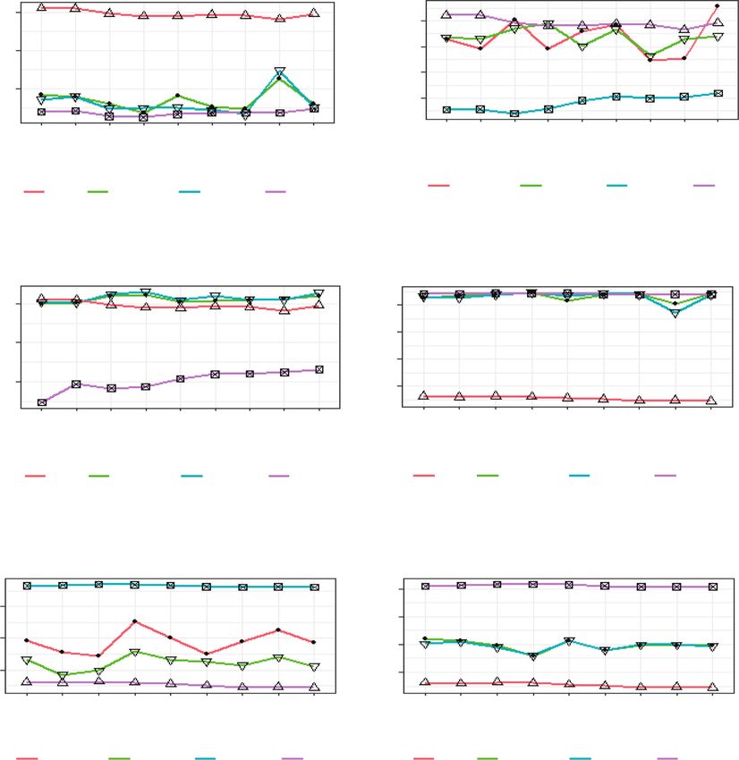
Further, this research applied out-of-sample evaluation. The estimation windows or                        Risk-based
optimization days for portfolio construction ranged from 120 to 360 days. For instance, the           optimization on
log-returns data set ranged from August 8, 2015 to October 20, 2020, and suppose the
optimization days were 360 days, meaning that this research used the date from August 8,
                                                                                                      cryptocurrencies
2015 to August 2, 2016 to obtain the weights and applied the weights on August 3, 2016. The
next optimization days were from August 9, 2015 to August 3, 2016, and it resulted in optimal
weights that applied the weights on August 4, 2016. The researcher repeated the process for
each new window created from the remaining sample. The researcher used daily sliding
windows in order to be comparable with the time-varying approach of GARCH. Also, the
researcher argued that frequent rebalancing could minimize estimation error.
   Moreover, this research applied the dynamic conditional correlation (DCC)-GARCH model
of Engle (2002) and asymmetric DCC (ADCC) of Cappiello et al. (2006). The dynamic variance-
covariance matrix:
                                       Vt ¼ Dt Rt Dt                                       (8)

Where Rt is a matrix of conditional correlation and Dt is a diagonal matrix for conditional
standard deviation
                                               1     1

                                  Dt ¼ diag v2n;t ; v2x;t                                (9)

                                   Rt ¼ diagðJt Þ−1=2 Jt diagðJt Þ−1=2                         (10)

The dynamics of J in the DCC process is
                                                                  0
                            Jt ¼ ð1  δ1  δ2 Þ J þ δ1 zt−1 zt−1 þ δ2 Jt−1                     (11)

Where J is the unconditional variance-covariance matrix of standardized residuals, δ1 is a
shock parameter and δ2 is the persistency variable. Cappiello et al. (2006) modify the DCC by
adding an asymmetric term
                        0          0        0           0     0          0     0   0
            Jt ¼ ðJ  P J P  Q J Q  R J − RÞ þ P zt−1 zt−1 P þ Q Jt−1 Q þ R z−t zt− R        (12)

A rolling window analysis created one-step-ahead dynamic covariances. The forecast length
was fixed at 1750 observations. However, the researcher also analysed the results from
various forecast lengths (see Figure 3). The GARCH models were refit starting at 120
observations. Every GARH refit defines how many times the model is recalculated and the
forecast duration is actually measured. For example, for a forecast length of 1,500 and refit
every 120 days, for a total actual forecast length of 1,500, there are 10 windows of 120
periods each.
   Moreover, this research also imposed 50 basis points of transaction cost (TCost). TCost is
the cost of purchasing or selling securities in order to construct a portfolio (Chavalle and
Chavez-Bedoya, 2019). The formula of TCost is (Platanakis et al., 2018):
                                       X N

                              TCostt ¼      Ta wa;t  wþa;t−1                          (13)
                                                a¼1

Where wþ a;t−1 represents the weight of the ath asset at the end of the period t – 1, and Ta is the
ath asset’s proportionate transaction expense.

3. Empirical results and discussions
This segment displays the effects of the creation of the portfolio. The first part of this section
concerns the analysis of results from stylized facts and the efficient frontier. The second part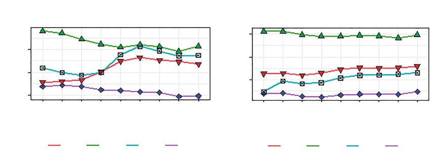
JCMS                                        Transaction Cost vs Sortino Ratio                                               Transaction Cost vs Sortino Ratio
                                                                                                                       1750 Days Forecast Length(Dynamic Approach)
                                                    Static Approach
                                   0.05

                                                                                                      Sortino
                                   0.00                                                                         0.00
                        Sortino
                                  –0.05
                                                                                                                –0.1
                                  –0.10
                                  –0.15                                                                         –0.2
                                  –0.20
                                                                                                                        10     20   30      40     50   60    70   80    90 100
                                  –0.25
                                           10   20    30   40    50    60    70    80    90 100                                Transaction Cost (Basis Points)
                                                Transaction Cost (Basis Points)
                                                                                                                          ERC-ADCC          EWP               MDP-DCC       MVP-DCC

                                                     ERC        EWP          MDP          MVP                             ERC-DCC           MDP-ADCC          MVP-ADCC

                                                                  (a)                                                                               (b)

                                               Transaction Cost vs Sortino Ratio                                             Transaction Cost vs Sortino Ratio
                                         1630 Days Forecast Length(Dynamic Approach)                                   1540 Days Forecast Length(Dynamic Approach)
                                   0.1

                                  0.00                                                                          0.00

                                                                                                      Sortino
                        Sortino

                                  –0.1                                                                          –0.1

                                  –0.2                                                                          –0.2

                                          10    20    30   40    50     60   70     80    90 100                        10     20      30   40     50   60    70   80    90 100
                                                 Transaction Cost (Basis Points)                                                Transaction Cost (Basis Points)

                                            ERC-ADCC       EWP               MDP-DCC        MVP-DCC                          ERC-ADCC        EWP              MDP-DCC       MVP-DCC

                                            ERC-DCC        MDP-ADCC          MVP-ADCC                                        ERC-DCC         MDP-ADCC         MVP-ADCC

                                                                 (c)                                                                                    (d)
Figure 3.              Note(s): These figures display portfolio performance concerning the Sortino ratio across different
Sortino ratio
vs transaction costs   transaction costs and forecast lengths of dynamic approaches. These portfolios applied 360 days
                       of optimization (static approach) and GARCH refits (dynamic method)

                       discusses the static method results, while the dynamic optimization results are in the last part
                       of this section.

                       3.1 Stylized fact
                       Table 1 presents descriptive statistics. All log-returns did not conform with normality
                       distribution, which was verified by the Shapiro-Wilk test. Interestingly, the returns were
                       positively skewed besides BTC, implying that buying assets with positive skewness could
                       lead to a sizeable positive return (Eraker and Wu, 2017). XEM had the highest mean returns,
                       and this finding is different from Antonakakis et al. (2019), who found that ETH had the
                       highest mean returns.
                          Also, XEM had the highest standard deviation, and this finding is different from Liu
                       (2019). XEM was the most risky crypto because it had the worst ES and VaR, while USDT
                       was the least risky crypto. Further, XEM had the best risk-adjusted return. Moreover, Phillips
                       and Perron (PP), augmented Dickey-Fuller (ADF) and Kwiatkowski, Phillips, Schmidt and
                       Shin (KPSS) tests showed that all returns were stationary. Also, all series were autocorrelated.
                       Hence, GARCH estimation is feasible.
                          Figure 4 shows the correlogram of daily log returns. Blue color shows a positive
                       correlation, while a red color reveals a negative correlation. The darker the color, the greater
                       the level of the correlations. The color becomes washed out when the correlations are near
                       zero. Findings show that most of the assets had positive correlations, consistent with Liu
                       (2019). Interestingly, USDT had a weak and negative correlation with other cryptos.
                          Also, Figure 5 presents an efficient frontier from a long-only portfolio. USDT and XEM
                       were located on the efficient frontier, indicating the lowest risk and the best-expected return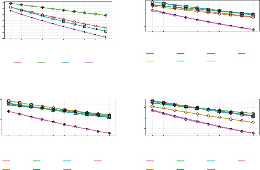
BTC      ETH             XRP             LTC             XLM             XMR            DASH            USDT             XEM             DOGE

Obs                  1901             1901          1901             1901             1901          1901           1901            1901            1901             1901
Min                0.464            0.551        0.616           0.449          0.410         0.494        0.459           0.049         0.362           0.493
Median(%)            0.206            0.000        0.230             0.000         0.200          0.000        0.080            0.000           0.000             0.000
Max                  0.225            0.412          1.027            0.510           0.723         0.585          0.438           0.057           0.996             0.518
Mean(%)              0.201            0.326          0.179            0.127           0.184         0.267          0.162           0.000           0.349             0.144
Std                  0.039            0.062          0.066            0.055           0.073         0.064          0.057           0.006           0.078             0.061
Skewness           0.096             0.079          2.960            0.764           2.000         0.678          0.636           0.288           1.974             1.034
Kurtosis            14.133            8.147         46.686           13.256          18.957         9.839          8.964          16.772          19.808           15.181
ES                 0.079            0.125        0.133           0.111          0.148         0.128        0.116           0.013         0.158           0.123
VaR                0.062            0.099        0.106           0.088          0.118         0.102        0.092           0.010         0.125           0.098
Drawdown             0.886            0.976          0.988            0.976           0.990         0.983          0.993           0.115           0.996             0.973
Omega                1.180            1.133          1.107            1.079           1.087         1.133          1.090           1.000           1.153             1.085
Sortino              0.071            0.051          0.047            0.036           0.042         0.064          0.043           0.000           0.075             0.037
Sharpe               0.051            0.037          0.027            0.023           0.025         0.042          0.028           0.000           0.045             0.024
KPSS                 0.063            0.081          0.092            0.108           0.096         0.093          0.099           0.007           0.106             0.046
PP                44.86***        43.28***     45.86***        44.20***        41.61***      46.19***     45.00***       82.99***       47.10***        41.64***
ADF               30.33***        28.88***     27.45***        30.62***        30.02***      31.43***     31.57***       39.86***       34.30***        28.61***
Shapiro-W            0.88***          0.90***        0.71***          0.85***         0.82***       0.90***        0.89***         0.66***         0.85***           0.81***
Note(s): This table presents descriptive stats of the log returns of the cryptos. Expected shortfall (ES) and value at risk (VaR) used 95% confidence level. ADF (PP) is
augmented Dickey-Fuller (Phillips and Perron) statistic. KPSS is Kwiatkowski, Phillips, Schmidt and Shin statistic. The Shapiro-Wilk is to test normality. *** Statistically
sig at 1 % level. The risk-free rate was assumed to be zero for the calculation of Sharpe and minimum acceptance return (MAR) of Sortino. A target threshold of zero was
also used in omega ratio
                                                                                                                                                                    Risk-based
                                                                                                                                                                optimization on
                                                                                                                                                                cryptocurrencies

             Table 1.
  Descriptive statistics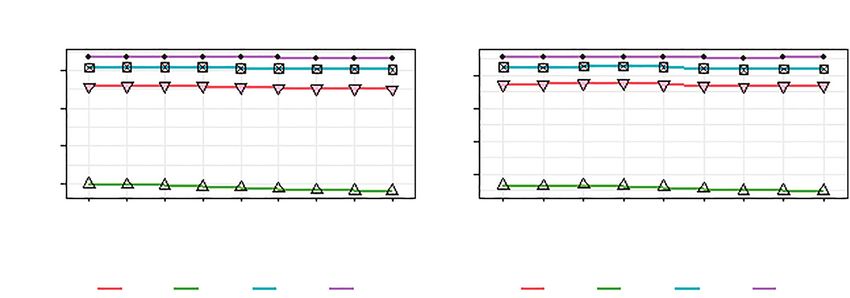
JCMS
DOGE
DASH
USDT
XMR
XEM
XRP
XLM
BTC
ETH
LTC
1
BTC
0.75
ETH
XRP 0.55
LTC
0.25
XLM
0
XMR
–0.25
DASH
USDT –0.05
XEM –0.75
DOGE
–1
Note(s): This figure shows correlogram matrix of the assets. The blue colour presents
Figure 4.
Correlogram
a positive correlation while red colour shows a negative correlation. The darker the
colour, the greater the level of the correlation
Efficient Frontier
0.004
XEM
ETH
0.003
Target Return [mean]
XMR
0.0012 0.0023
0.002
BTC
EWT XRP XLM
DASH
DOGE
LTC
0.001
0.000
Rmetrics
USDT
0.00 0.02 0.04 0.06 0.08
Target Risk [Sigma]
Note(s): This figure presents efficient frontier from short-selling constrained mean-variance
portfolio. The x and y-axis are in percentage. This figure consists of efficient frontier, tangency
line and EWP which is the naïve strategy. The line of Sharpe ratio (yellow) which coincides with
Figure 5.
Efficient frontier tangency point of the portfolio is also shown. The right hand side axis of the figure represents the
range of Sharpe ratio
among other cryptos. Moreover, Figure 5 displays in-sample analysis, implying that the
covariance matrix was estimated based on the entire sample, which was not a realistic
perspective. In-sample analysis is mainly used as a theoretical perspective rather than a
practical perspective (Liu, 2019; Schellinger, 2020). Therefore, this paper focused on out-of-
sample analysis using the rolling windows method.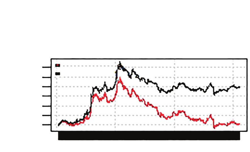
3.2 Static approach                                                                                                                      Risk-based
This section shows MVP, MDP and ERC portfolios’ optimization results based on a static                                               optimization on
covariance matrix. Figure 6 shows optimal weights from static portfolios. The highest
proportion of assets in the portfolio was USDT for all optimization methods. The average
                                                                                                                                     cryptocurrencies
proportions of USDT for MVP, ERC and MDP portfolio were 0.971, 0.697 and 0.832,
respectively. Interestingly, the lowest proportion of assets in the portfolio was XMR for MVP
and MDP portfolios. It was XLM for the ERC approach.
   Further, Table 2 shows the performance evaluation of MDP, ERC and MVP portfolios.
Panel A exhibits the performance without transaction cost, while Panel B shows the
performance with transaction cost (50 basis points). Without transaction costs, the level of
risk (ES and VaR) of MDP, ERC and MVP portfolios was significantly lower than individual
crypto (see Table 1). Interestingly, the level of risk was still reduced considerably after
imposing transaction cost to the portfolio. Moreover, the portfolio’s risk-adjusted return was
not significantly greater than individual cryptos, indicating that diversification across
cryptos did not significantly enhance return. This finding is different from Liu (2019). Note
that Table 2 only shows the performance of static MVP, ERC and MDP portfolio under 120,
150 and 180 estimation days. One should refer to Figures 1 and 2 for various estimation days.
   Figures 1 and 2 display portfolio performance (Sortino and ES) across different
optimization days [1]. Without transaction costs, the MDP portfolio was the best strategy in
terms of the Sortino ratio. After considering transaction costs, EWP outperformed other
portfolios regarding the Sortino ratio. In the level of risk or expected shortfall (Figure 2), EWP
was the worst performer (with and without transaction cost), while static MVP was the least
risky strategy.

                   Optimal Weights-MVP-Static Approach                                   Optimal Weights-MDP-Static Approach
           1.00                                                                 1.00

           0.75                                                                 0.75
 Weights

                                                                      Weights

           0.50                                                                 0.50

           0.25                                                                 0.25

           0.00                                                                 0.00
                  2017    2018               2019    2020                               2017    2018       2019      2020
                                   Date                                                                  Date

                   BTC      DOGE              LTC     XEM      XMR                       BTC      DOGE      LTC      XEM       XMR

                   DASH     ETH               USDT    XLM      XRP                       DASH     ETH       USDT     XLM       XRP

                                                       Optimal Weights-ERC-Static Approach
                                             1.00

                                             0.75
                                   Weights

                                             0.50

                                             0.25

                                             0.00
                                                     2017     2018              2019    2020
                                                                       Date

                                                      BTC      DOGE              LTC     XEM     XMR

                                                      DASH     ETH               USDT    XLM     XRP
                                                                                                                                                Figure 6.
                                                                                                                                       Optimal weights of
 Note(s): These figures exhibit optimal weights from MVP, MDP, and ERC portfolio. The                                                     static approach
 optimization days were 360 days with short-selling constraints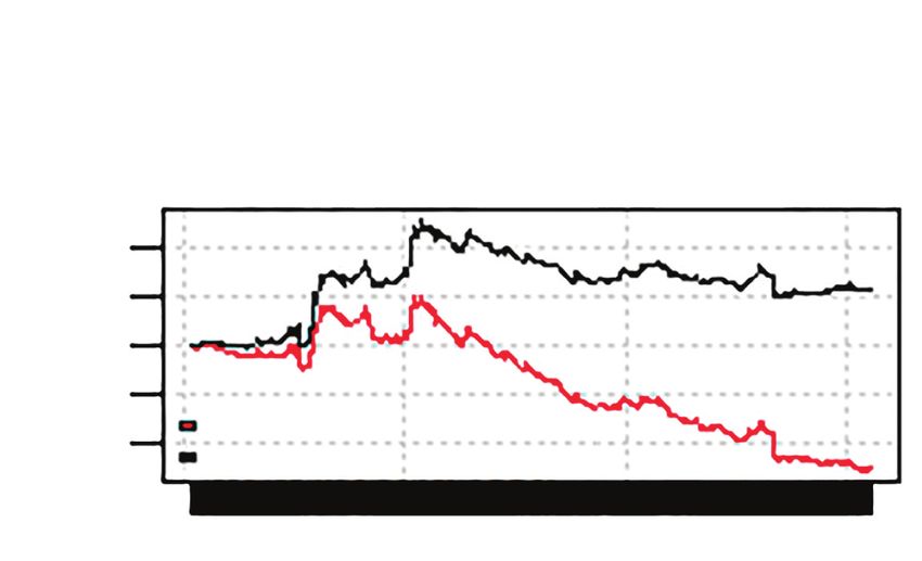
JCMS
approach
Table 2.
Performance
evaluation-static
Optimization 120 days Optimization 150 days Optimization 180 days
MVP ERC MDP MVP ERC MDP MVP ERC MDP
Panel A
ES (%) 1.276 2.846 0.792 1.284 2.840 1.847 1.302 2.832 1.849
VaR (%) 1.015 2.263 0.628 1.021 2.258 1.468 1.036 2.252 1.469
Drawdown (%) 12.700 82.400 7.970 14.400 80.680 46.830 15.500 80.380 47.630
Omega 1.077 1.077 1.258 1.079 1.077 1.091 1.075 1.079 1.085
Sortino (%) 2.761 3.124 7.487 2.889 3.212 3.979 2.776 3.331 3.758
Sharpe (%) 1.887 2.219 4.430 1.970 2.283 2.690 1.885 2.360 2.531
Panel B
ES (%) 2.466 3.293 2.118 2.478 3.279 2.777 2.441 3.241 2.742
VaR (%) 1.990 2.646 1.708 1.999 2.635 2.235 1.971 2.605 2.207
Drawdown (%) 88.815 86.581 38.767 88.961 86.908 86.118 88.766 86.241 85.675
Omega 0.583 0.780 0.684 0.585 0.782 0.704 0.559 0.772 0.686
Sortino (%) 13.087 8.639 12.701 12.930 8.610 10.311 13.657 9.025 10.867
Sharpe (%) 10.040 6.355 9.179 9.915 6.363 7.622 10.679 6.734 8.158
Note(s): This table exhibits performance measurement of MVP, ERC and MDP portfolio with different estimation windows (120, 150 and 180 days). Panel A shows the
performance without transaction cost, while Panel B indicates the performance with transaction cost (50 basis points). The risk-free rate was assumed to be zero for the
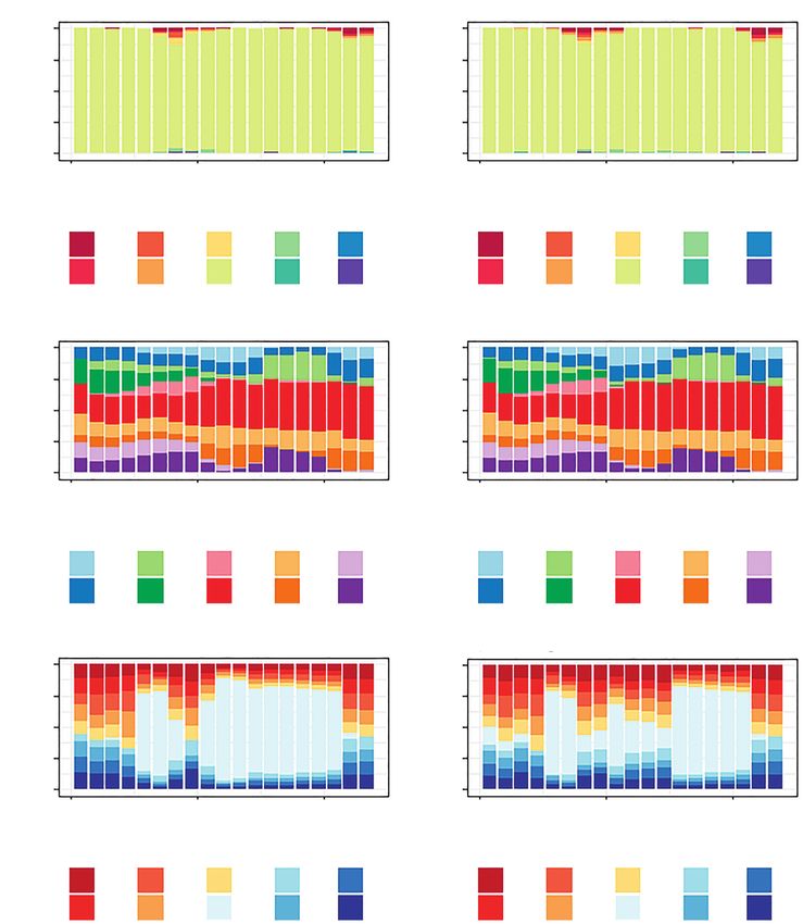
calculation of Sharpe and minimum acceptance return (MAR) of Sortino. A target threshold of zero was also used in omega ratioUnlike previous studies, this research computed cumulative returns. Figure 7 presents the Risk-based
cumulative returns of the portfolios (static approach). Based on the statistics, EWP was less optimization on
affected by transaction costs, and this finding is similar to Liu (2019). EWP had positive
average of net cumulative returns, while MVP, MDP and ERC had negative average of net
cryptocurrencies
cumulative returns.
3.3 Dynamic approach
Before applying the optimization, the researcher implemented diagnostic tests. Table 3
displays results of diagnostic tests. This paper used GARCH (1,1). Table 3 shows three
coefficients from the variance equation. The omega is the intercept, while alpha (1) and beta
(1) are the first lag of squared returns and conditional variance, respectively. The sum of α (1)
and β (1) was less than one and significant, indicating that the series was mean-reverting.
Moreover, the Ljung-Box tests exhibit that the GARCH estimation could obtain all returns
volatility since autocorrelation did not exist in the standardized residuals. Hence, the GARCH
(1,1) in this research is fit.
Further, Figure 8 displays the optimal weights of the dynamic approach. The
models’ settings were the rolling windows method with 1,750 days of forecast length
and 360 days of GARCH refits. Similar to the static process, USDT had immense
weight in the portfolio. However, the average of USDT’s weight in the dynamic ERC
and MDP portfolio is noticeably different from the static portfolio. For instance, the
average weight of USDT in ERC-ADCC and ERC-DCC portfolios were 40 percent and
33 percent, respectively. The mean weight of USDT in MDP-ADCC and MDP-DCC
Cumulative Returns-MVP Cumulative Returns-MDP
1.0
return
return
–0.5
0.0
–1.0
With Transaction Cost With Transaction Cost
–1.5
No Transaction Cost No Transaction Cost
08-2016
11-2016
01-2017
04-2017
07-2017
10-2017
01-2018
04-2018
07-2018
10-2018
01-2019
04-2019
07-2019
10-2019
01-2020
03-2020
06-2020
09-2020
08-2016
11-2016
01-2017
04-2017
07-2017
10-2017
01-2018
04-2018
07-2018
10-2018
01-2019
04-2019
07-2019
10-2019
01-2020
03-2020
06-2020
09-2020
date date
Cumulative Returns-ERC Cumulative Returns-EWP
3.0
1.0
With Transaction Cost
No Transaction Cost
return
return
–1.0 0.0
1.5
With Transaction Cost
0.0
No Transaction Cost
08-2016
11-2016
01-2017
04-2017
07-2017
10-2017
01-2018
04-2018
07-2018
10-2018
01-2019
04-2019
07-2019
10-2019
01-2020
03-2020
06-2020
09-2020
08-2016
10-2016
01-2017
04-2017
07-2017
10-2017
01-2018
04-2018
07-2018
10-2018
01-2019
04-2019
07-2019
10-2019
01-2020
03-2020
06-2020
09-2020
date date
Note(s): These figures exhibit cumulative returns of MVP, ERC, MDP, and EWP portfolio. Figure 7.
Cumulative returns –
The black line represents a portfolio without transaction cost, while the red line indicates a static approach
portfolio with transaction cost (50 bps). The optimization days were 360JCMS Estimate t-value
Ω 0.011 3.783***
α (1) 0.154 5.796***
β (1) 0.805 23.892***
Information criterion stats
AIC 1.124
BIC 1.133
SIC 1.124
HQIC 1.128
Log-likelihood 1106.876
Standardised residuals tests
Statistic p-value
Ljung-Box test (Q10) 9.988 0.442
Ljung-Box test (Q15) 16.888 0.326
Ljung-Box test (Q10)-squared 9.159 0.517
Ljung-Box test (Q15)-squared 16.336 0.360
LM arch test 9.884 0.626
Table 3. Note(s): This table exhibits diagnostic test of GARCH (1,1). The coefficients in the variance equation are listed,
Diagnostic tests Ω, α (1) and β (1). *** Statistically sig at 1%
portfolios were 32% and 33%, respectively. Interestingly, BTC had the second-largest
weight in the dynamic ERC portfolio, while XEM had the second-largest weight in the
dynamic MDP portfolio.
Furthermore, Table 4 indicates the performance evaluation of dynamic MVP, ERC and
MDP portfolio. Panel A shows the performance without transaction cost, while Panel B
indicates the performance with transaction cost (50 basis points). Without transaction cost,
dynamic MVP had the lowest portfolio risk level, followed by a dynamic MDP portfolio
(based on ES approach). Moreover, the ERC strategy was the most risky approach. With
transaction cost, dynamic MDP was the best performer concerning the Sortino and
Omega ratio.
Interestingly, the transaction cost could decrease the dynamic portfolio’s risk under
dynamic ERC and MDP models. This finding implied that frequent rebalancing might result
in higher mean returns without significantly increasing risk, and this finding is consistent
with a previous study (Brauneis and Mestel, 2019). Note that Table 4 only shows the
performance of dynamic MVP, ERC and MDP portfolio under 120, 150 and 180 GARCH refits
days. One should refer to Figure 9 for various GARCH refit days.
Moreover, Figure 10 shows cumulative returns from dynamic portfolios. With and
without transaction cost, dynamic MDP had the highest mean of cumulative returns, followed
by dynamic ERC. The average cumulative returns from the dynamic portfolios were higher
than the average from the static portfolios. However, the average cumulative return from the
EWP portfolio (see Figure 7) was slightly lower than the dynamic MDP, which had the
highest mean of cumulative returns under dynamic strategies.
Further, Figure 9 presents the Sortino ratio’s comparison between static and
dynamic MVP, ERC and MDP optimization. The results of Figure 9 included 50 basis
points of transaction costs. Regarding the Sortino ratio, dynamic MDP (Figure 9C) was
the best strategy. Intriguingly, dynamic MDP could win over naı€ve system in most of
GARCH refits days. The second-best strategy was dynamic ERC. Dynamic ERC
(Figure 9B) could also beat the 1/N method, although it was inconsistent under various1.00
Optimal Weights-MVP-ADCC
1.00
Optimal Weights-MVP-DCC
Risk-based
optimization on
0.75 0.75
cryptocurrencies
Weights
Weights
0.50 0.50
0.25 0.25
0.00 0.00
2016 2018 2020 2016 2018 2020
Date Date
BTC DOGE LTC XEM XMR BTC DOGE LTC XEM XMR
DASH ETH USDT XLM XRP DASH ETH USDT XLM XRP
Optimal Weights-MDP-ADCC Optimal Weights-MDP-DCC
1.00 1.00
0.75 0.75
Weights
Weights
0.50 0.50
0.25 0.25
0.00 0.00
2016 2018 2020 2016 2018 2020
Date Date
BTC DOGE LTC XEM XMR BTC DOGE LTC XEM XMR
DASH ETH USDT XLM XRP DASH ETH USDT XLM XRP
Optimal Weights-ERC-ADCC Optimal Weights-ERC-DCC
1.00 1.00
0.75 0.75
Weights
Weights
0.50 0.50
0.25 0.25
0.00 0.00
2016 2018 2020 2016 2018 2020
Date Date
BTC DOGE LTC XEM XMR BTC DOGE LTC XEM XMR
DASH ETH USDT XLM XRP DASH ETH USDT XLM XRP
Note(s): These figures show optimal weights from MVP, MDP, and ERC portfolio based on
DCC-GARCH (1,1) and ADCC-GARCH (1,1) with multivariate Student’-t-distribution and Figure 8.
Optimal weights of
rolling windows method with 1750 days of forecast length. The GARCH models were refit dynamic approach
every 360 days
refit days. However, Figure 9 only shows the performance of dynamic MVP, ERC and
MDP portfolio under 1750 days of forecast length. One should refer to Figure 3 for
various forecast lengths.
Moreover, Figure 9 also shows the expected shortfall’s (ES) comparison between
static and dynamic MVP, ERC and MDP optimization. Concerning ES, none of the
dynamic strategies could beat static strategies. The static MVP (Figure 9D) was the
least risky strategy. Interestingly, the 1/N approach was the most risky strategy. TheJCMS Refit days ES VaR Drawdown Omega Sortino Sharpe
Panel A
MVP-ADCC 120 0.014 0.011 0.357 1.080 0.028 0.019
MVP-DCC 0.014 0.011 0.371 1.122 0.043 0.028
ERC-ADCC 0.052 0.041 0.724 1.198 0.068 0.051
ERC-DCC 0.063 0.050 0.871 1.145 0.051 0.038
MDP-ADCC 0.061 0.049 0.978 1.217 0.098 0.066
MDP-DCC 0.061 0.049 0.959 1.213 0.096 0.065
MVP-ADCC 150 0.014 0.011 0.456 1.091 0.032 0.021
MVP-DCC 0.015 0.012 0.377 1.140 0.050 0.031
ERC-ADCC 0.064 0.051 0.783 1.109 0.039 0.029
ERC-DCC 0.067 0.053 0.853 1.141 0.052 0.038
MDP-ADCC 0.061 0.048 0.942 1.203 0.092 0.062
MDP-DCC 0.062 0.049 0.927 1.206 0.093 0.063
MVP-ADCC 180 0.015 0.012 0.326 1.150 0.051 0.033
MVP-DCC 0.013 0.011 0.374 1.174 0.062 0.039
ERC-ADCC 0.061 0.048 0.684 1.240 0.087 0.062
ERC-DCC 0.066 0.053 0.775 1.174 0.064 0.047
MDP-ADCC 0.062 0.049 0.975 1.214 0.097 0.065
MDP-DCC 0.061 0.048 0.988 1.211 0.096 0.065
Panel B
MVP-ADCC 120 0.027 0.022 0.864 0.662 0.108 0.079
MVP-DCC 0.027 0.022 0.877 0.644 0.115 0.085
ERC-ADCC 0.050 0.040 0.894 0.953 0.018 0.013
ERC-DCC 0.057 0.046 0.944 0.956 0.017 0.012
MDP-ADCC 0.048 0.038 0.895 1.000 0.000 0.000
MDP-DCC 0.048 0.038 0.886 1.004 0.002 0.001
MVP-ADCC 150 0.026 0.021 0.871 0.638 0.115 0.085
MVP-DCC 0.027 0.022 0.865 0.658 0.110 0.110
ERC-ADCC 0.058 0.047 0.966 0.880 0.048 0.036
ERC-DCC 0.061 0.049 0.964 0.940 0.024 0.018
MDP-ADCC 0.049 0.039 0.892 1.004 0.002 0.001
MDP-DCC 0.049 0.039 0.889 1.008 0.003 0.002
MVP-ADCC 180 0.026 0.021 0.887 0.619 0.120 0.091
MVP-DCC 0.026 0.021 0.894 0.604 0.126 0.126
ERC-ADCC 0.056 0.044 0.903 1.002 0.001 0.000
ERC-DCC 0.060 0.048 0.944 0.982 0.007 0.005
MDP-ADCC 0.050 0.040 0.889 1.022 0.010 0.006
MDP-DCC 0.051 0.041 0.884 1.029 0.012 0.008
Note(s): This table exhibits performance measurement of dynamic MVP, ERC and MDP portfolio with
different number of GARCH refits (120, 150 and 180 days). Panel A shows the performance without transaction
cost, while Panel B indicates the performance with transaction cost (10 basis points). The time-varying
Table 4. covariances were obtained from DCC-GARCH (1,1) and ADCC-GARCH (1,1) with multivariate Student’s
Performance t-distribution. Rolling windows method with 1,750 days of forecast length was employed. The risk-free rate was
evaluation-dynamic assumed to be zero for the calculation of Sharpe and minimum acceptance return (MAR) of Sortino. A target
approach threshold of zero was also used in omega ratio
static MDP (Figure 9F) was the second-least risky approach. Moreover, the findings
were also in line with previous literature that stated σ MVP≤σ ERC≤σ EWP (Maillard
et al., 2010).
Figure 3 exhibits the Sortino ratio across different transaction costs and forecast
lengths. Note that the results displayed in Figure 3 used 360 days of estimation windows
and GARCH refit. Figure 3A indicates that EWP outperformed all static portfolios. Also,
static MVP was the worst performer regarding the Sortino ratio across differentMVP-Dynamic vs Static (Sortino Ratio)
With Transaction Cost
ERC-Dynamic vs Static (Sortino Ratio)
With Transaction Cost
Risk-based
0.00
0.000
optimization on
cryptocurrencies
Sortino
Sortino
–0.05 –0.025
–0.050
–0.10
–0.075
120 150 180 210 240 270 300 330 360 120 150 180 210 240 270 300 330 360
Optimization(Static) / Refit(Dynamic) days Optimization(Static) / Refit(Dynamic) days
ERC-ADCC ERC-DCC ERC-Static EWP
EWP MVP-ADCC MVP-DCC MVP-Static
(a) (b)
MDP-Dynamic vs Static (Sortino Ratio) MVP-Dynamic vs Static (Sortino Ratio)
With Transaction Cost With Transaction Cost
0.00 ES in % –3
–4
–0.05
Sortino
–5
–0.10 –6
120 150 180 210 240 270 300 330 360 120 150 180 210 240 270 300 330 360
Optimization(Static) / Refit(Dynamic) days Optimization(Static) / Refit(Dynamic) days
EWP MDP-ADCC MDP-DCC MDP-Static EWP MVP-ADCC MVP-DCC MVP-Static
(c) (d)
ERC-Dynamic vs Static (Sortino Ratio) MDP-Dynamic vs Static (Sortino Ratio)
With Transaction Cost With Transaction Cost
–3
–4
ES in %
–4
ES in %
–5 –5
–6 –6
120 150 180 210 240 270 300 330 360 120 150 180 210 240 270 300 330 360
Optimization(Static) / Refit(Dynamic) days Optimization(Static) / Refit(Dynamic) days
ER-ADCC ERC-DCC ERC-Static EWP EWP MDP-ADCC MDP-DCC MDP-Static
(e) (f)
Note(s): These figures exhibit a comparison between static and dynamic MVP, MDP, and ERC portfolio. The Figure 9.
static approach used sample covariance or correlation matrix while the dynamic system used covariances from Dynamic vs static
DCC-GARCH (1,1) and ADCC-GARCH (1,1) with multivariate Student's t distribution. The transaction cost approach
was 50 bps. The forecast length for dynamic models was 1750 days
transaction costs. These findings are consistent with Liu (2019). Moreover, there are two
interesting findings in Figure 3B. Firstly, dynamic MVP was still the worst performer for
the Sortino ratio across different transaction costs. Secondly, only dynamic ERC and
MDP could beat the naı€ve strategy, although it was not consistent across many
transaction costs. Dynamic MDP could win the naı€ve approach when the transaction
costs ranged from 10 to 50 bps. However, Figures 3C and 3D display different results
under different forecast lengths. Figure 3C shows that dynamic ERC could win the naı€ve
approach when the transaction costs ranged from 10 to 60 bps, while Figure 3D indicates
that only ERC-ADCC and dynamic MDP could win the naı€ve approach when the
transaction costs ranged from 10 to 40 bps. Dynamic MVP had the worst risk-adjusted
performance in Figures 3C and 3D.JCMS Cumulative Returns-MVP-ADCC Cumulative Returns-MVP-DCC
–1.5 –0.5 0.5
–2.0 –1.0 0.0
return
return
With Transaction Cost With Transaction Cost
No Transaction Cost No Transaction Cost
01-2016
04-2016
07-2016
02-2017
05-2017
09-2017
12-2017
03-2018
07-2018
10-2018
01-2019
05-2019
08-2019
03-2020
06-2020
09-2020
11-2016
11-2019
01-2016
04-2016
07-2016
02-2017
05-2017
09-2017
12-2017
03-2018
07-2018
10-2018
01-2019
05-2019
08-2019
03-2020
06-2020
09-2020
11-2016
11-2019
date date
Cumulative Returns-MDP-ADCC Cumulative Returns-MDP-DCC
With Transaction Cost With Transaction Cost
3.0
3.0
No Transaction Cost No Transaction Cost
return
return
1.5
1.5
0.0
0.0
01-2016
04-2016
07-2016
02-2017
05-2017
09-2017
12-2017
03-2018
07-2018
10-2018
01-2019
05-2019
08-2019
03-2020
06-2020
09-2020
11-2016
11-2019
01-2016
04-2016
07-2016
02-2017
05-2017
09-2017
12-2017
03-2018
07-2018
10-2018
01-2019
05-2019
08-2019
03-2020
06-2020
09-2020
11-2016
11-2019
date date
Cumulative Returns-ERC-ADCC Cumulative Returns-ERC-DCC
3
With Transaction Cost
3.0
No Transaction Cost
–1 0 1 2
return
return
1.5
With Transaction Cost
0.0
No Transaction Cost
01-2016
04-2016
07-2016
02-2017
05-2017
09-2017
12-2017
03-2018
07-2018
10-2018
01-2019
05-2019
08-2019
03-2020
06-2020
09-2020
11-2016
11-2019
01-2016
04-2016
07-2016
02-2017
05-2017
09-2017
12-2017
03-2018
07-2018
10-2018
01-2019
05-2019
08-2019
03-2020
06-2020
09-2020
11-2016
11-2019
date date
Note(s): These figures exhibit the cumulative return of MVP, MDP, and ERC portfolio using DCC-
Figure 10.
GARCH (1,1) and ADCC-GARCH (1,1) with multivariate Student’s t distribution. The black line
Cumulative return-
dynamic approach represents a portfolio without transaction cost, while the red line indicates a portfolio with transaction
cost (50 bps). GARCH refits days were 360
4. Robustness tests
The robustness test is the last part of the empirical results section of this research. There
were two types of robustness tests in this study. First, the researcher used another
researcher’s sample (Schellinger, 2020). Second, the researcher applied extension models of
DCC and ADCC which were VAR-DCC and VAR-ADCC (Yousaf and Ali, 2020b). As stated
earlier, this research used ten blended cryptocurrencies. A previous study (Schellinger,
2020) divided the cryptos into coins (BTC, IOTA, ETH, EOS, XRP, NEO, LTC, BCH, XLM,
DASH) and tokens (MAID, USDT, GNT, GAS, OMG, DGD, BAT, PPT, SNT, REP). Global
minimum variance (GMV) strategy was the best performer in regars to risk-adjusted return.
Hence, this research’s robustness check used the sample and study period of the previous
study and set GMV as the benchmark to beat. The sampling started from August 1, 2017, to
May 31, 2019.Before applying dynamic optimization, the researcher created efficient frontiers of long- Risk-based
only constrained mean-variance portfolio from token and coin-type cryptos (Figure 11). The optimization on
left-hand side of the figure shows an efficient frontier from coin-type cryptocurrency. BTC
and DASH are located on the efficient frontier indicating the lowest risk and the best-expected
cryptocurrencies
return among other cryptos. Moreover, the right-hand side of the figure shows an efficient
frontier from token-type cryptocurrency. BAT and USDT are located on the efficient frontier
indicating the lowest risk and the best-expected return among other cryptos.
Table 5 shows the results of the robustness test. For coin-type cryptos, all dynamic
strategies outperformed the benchmark. While GMV’s Sharpe annualized was marginally
better than Sharpe annualized from the dynamic process, the Sortino and omega ratios are
better measurements due to their ability to capture a downward deviation (Sortino and Price,
1994; Keating and Shadwick, 2002). More interestingly, dynamic ERC and MDP yielded a
Efficient Frontier Efficient Frontier
Traget Return[mean]
Traget Return[mean]
0.0299 0.034
0.0804 0.126
0.0
0.05
Rmetrics
Rmetrics
–0.2
–0.10
0 2 4 6 8 0 2 4 6 8
Traget Risk[Sigma] Traget Risk[Sigma]
Note(s): These figures present efficient frontiers from long-only constrained mean-variance
portfolios. The x and y-axis are in percentages. These figures consist of the efficient frontier,
tangency line, and EWP, which is the naïve strategy. The Sharpe ratio line (yellow), which
coincides with the portfolio’s tangency point, is also in the figure. The right-hand side axis
of the model represents the range of the Sharpe ratio. The left-hand side of the figure shows Figure 11.
Efficient frontiers-
an efficient frontier from coin-type cryptocurrencies. The right-hand side of the figure robustness test
offers an efficient frontier from token-type cryptocurrencies
Coin-type cryptos Token-type cryptos
Strategies Sortino Omega Sharpe.Annualized Sortino Omega Sharpe.Annualized
GMV 0.0086 1.0215 0.4956 0.0483 0.9400 0.6755
MVP-ADCC 0.0085 1.0215 0.4957 0.0169 0.9907 3.2830
VAR-MVP-ADCC 0.0059 0.9916 0.4969 0.0199 0.9832 3.2585
MVP-DCC 0.0059 0.9916 0.4969 0.0125 1.0013 3.2588
VAR-MVP-DCC 0.0095 1.0230 0.4486 0.0199 0.9832 3.2585
ERC-ADCC 0.0094 1.0228 0.4487 0.0279 0.9424 0.7384
VAR-ERC-ADCC 0.0094 1.0228 0.4487 0.0263 0.9462 0.7862
ERC-DCC 0.0095 1.0230 0.4486 0.0451 0.9048 0.7344
VAR-ERC-DCC 0.0048 0.9934 0.4437 0.0383 0.9190 0.7695
MDP-ADCC 0.0048 0.9935 0.4436 0.0190 0.9637 0.6397
VAR-MDP-ADCC 0.0051 0.9928 0.4409 0.0250 0.9508 0.6459
MDP-DCC 0.0051 0.9928 0.4409 0.0190 0.9637 0.6432
VAR-MDP-DCC 0.0086 1.0215 0.4956 0.0244 0.9520 0.6463
Note(s): This table exhibits performance evaluations of dynamic MVP, ERC and MDP portfolio against GMV
(Schellinger, 2020). The models applied DCC and ADCC-GARCH(1,1) with multivariate Student t and 40 days of Table 5.
GARCH refits. Following Schellinger (2020), the risk-free rate was 2.28% p.a, The rate was for calculating Performance
Sharpe and minimum acceptance return (MAR) of Sortino, while the Omega ratio’s target threshold used evaluation-
zero value robustness testJCMS positive Sortino ratio compared with other strategies. For token-type cryptos, all dynamic
system also outperformed the benchmark. Moreover, VAR-based models did not provide
significant portfolio risk-adjusted performance compared with non-VAR models. However,
VAR-based models could also win the benchmark. Overall, the dynamic MDP and ERC were
the best strategies. Note that the robustness test applied 40 days of GARCH refits in the
optimization [2]. The results of this study support the finding of a research by Inci and
Lagasse (2019) who used an earlier time-series sample that Bitcoin is feasible for
cryptocurrencies diversification.
5. Conclusion
This research aimed to present dynamic optimization on MVP, ERC and MDP. This
study applied dynamic covariances from multivariate GARCH (1,1) with the Student’s
t-distribution. This research also constructed static optimization from the conventional MVP,
ERC and MDP as the comparison. Moreover, this research applied the rolling windows
method with different GARH refits and forecast lengths to ensure out of sample analysis.
Findings showed that diversification across cryptos could lower the risk under expected
shortfall and VaR. MVP was the least risky strategy under static and dynamic approaches.
However, none of the portfolios under the static process could beat the naı€ve system when the
transaction cost more than 60 bps was imposed. Although dynamic portfolios outperformed
static portfolios concerning Sortino and omega ratios, dynamic portfolios were riskier than
the static approach.
Moreover, this research also created simulation regarding portfolio performance across
different transaction costs and forecast lengths. None of the portfolio strategies could
consistently outperform the 1/N approach under different schemes: net cumulative returns,
various estimation windows and forecast lengths. To further validate the findings, this study
used another researcher’s sample as a robustness check. Results showed that the dynamic
approach could beat another researcher’s best strategy: GMV. Notably, dynamic MDP and
ERC were the most consistent methods of outperforming 1/N system and the GMV under
certain schemes.
Although this paper has some interesting findings, still this paper is not without its
drawbacks. First, this paper only focuses on three risk-based portfolios, while there are still
other risks based methods such as inverse volatility, risk-efficient portfolios and maximum
decorrelation. Second, this paper uses dynamic covariances for ERC and MVP approaches
while applying dynamic correlation may result in better performance. Third, GARCH
estimations have been extensively researched. The validity of the findings under alternative
methods is left for future research. Lastly, the models seem too complicated to retail investors.
This study also paves the way for future research. For instance, a dynamic approach can
be applied to other, less risky assets such as stocks and bonds. Since this study only used one
portfolio constraint, future study can apply more than one portfolio constraint and objective.
Also, future studies can make comparisons between complicated method (e.g. GARCH-based
portfolio) and simple method (e.g. momentum-based portfolio).
ORCID iDs
Bayu Adi Nugroho http://orcid.org/0000-0001-6113-9362
Notes
1. The same conclusion is obtained from omega ratio and VaR.
2. Since the sample period is shorter, shorter GARCH refits days is required.References Risk-based
Ahmad, W., Sadorsky, P. and Sharma, A. (2018), “Optimal hedge ratios for clean energy equities”, optimization on
Economic Modelling, Vol. 72, pp. 278-295, doi: 10.1016/j.econmod.2018.02.008.
cryptocurrencies
Antonakakis, N., Chatziantoniou, I. and Gabauer, D. (2019), “Cryptocurrency market contagion:
market uncertainty, market complexity, and dynamic portfolios”, Journal of International
Financial Markets, Institutions and Money, Vol. 61, pp. 37-51, doi: 10.1016/j.intfin.2019.
02.003.
Antonakakis, N., Cunado, J., Filis, G., Gabauer, G. and de Gracia, F.P. (2020), “Oil and asset
classes implied volatilities: investment strategies and hedging effectiveness”, Energy
Economics, Vol. 91, 104762, doi: 10.1016/j.eneco.2020.104762.
Ardia, D., Bolliger, G., Boudt, K. and Gagnon-Fleury, J.-P. (2017a), “The impact of covariance
misspecification in risk-based portfolios”, Annals of Operations Research, Vol. 254 No. 1,
pp. 1-16, doi: 10.1007/s10479-017-2474-7.
Ardia, D., Boudt, K. and Gagnon-Fleury, J.-P. (2017b), “RiskPortfolios: computation of risk-based
portfolios in R”, The Journal of Open Source Software, Vol. 2 No. 10, p. 171, doi: 10.21105/
joss.00171.
Basher, S.A. and Sadorsky, P. (2016), “Hedging emerging market stock prices with oil, gold, VIX, and
bonds: a comparison between DCC, ADCC and GO-GARCH”, Energy Economics, Vol. 54,
pp. 235-247, doi: 10.1016/j.eneco.2015.11.022.
Baur, D.G. and Dimpfl, T. (2018), “Asymmetric volatility in cryptocurrencies”, Economics Letters,
Vol. 173, pp. 148-151, doi: 10.1016/j.econlet.2018.10.008.
Bouri, E., Lucey, B. and Roubaud, D. (2020), “Cryptocurrencies and the downside risk in equity
investments”, Finance Research Letters, Vol. 33, doi: 10.1016/j.frl.2019.06.009.
Brauneis, A. and Mestel, R. (2019), “Cryptocurrency-portfolios in a mean-variance framework”,
Finance Research Letters, Vol. 28, pp. 259-264, doi: 10.1016/j.frl.2018.05.008.
Cappiello, L., Engle, R. and Sheppard, K. (2006), “Asymmetric dynamics in the correlations of global
equity and bond returns”, Journal of Financial Econometrics, Vol. 4 No. 4, pp. 537-572, doi: 10.
1093/jjfinec/nbl005.
Chavalle, L. and Chavez-Bedoya, L. (2019), “The impact of transaction costs in portfolio optimization:
a comparative analysis between the cost of trading in Peru and the United States”, Journal of
Economics, Finance and Administrative Science, Vol. 24 No. 48, pp. 288-311, doi: 10.1108/JEFAS-
12-2017-0126.
Choueifaty, Y. and Coignard, Y. (2008), “Toward maximum diversification”, The Journal of Portfolio
Management, Vol. 35 No. 1, pp. 40-51, doi: 10.3905/JPM.2008.35.1.40.
Choueifaty, Y., Froidure, T. and Reynier, J. (2013), “Properties of the most diversified portfolio”,
Journal of Investment Strategies, Vol. 2 No. 2, pp. 1-22.
DeMiguel, V., Garlappi, L. and Uppal, R. (2007), “Optimal versus naive diversification: how inefficient
is the 1/N portfolio strategy?”, The Review of Financial Studies, Vol. 22 No. 5, pp. 1915-1953,
doi: 10.1093/rfs/hhm075.
Engle, R. (2002), “Dynamic conditional correlation: a simple class of multivariate generalized
autoregressive conditional heteroskedasticity models”, Journal of Business and Economic
Statistics, Vol. 20 No. 3, pp. 339-350, doi: 10.1198/073500102288618487.
Eraker, B. and Wu, Y. (2017), “Explaining the negative returns to volatility claims: an equilibrium
approach”, Journal of Financial Economics, Vol. 125 No. 1, pp. 72-98, doi: 10.1016/j.jfineco.2017.
04.007.
Ghalanos, A. (2019), rmgarch: Multivariate GARCH Models, R package version 1.3-7.
Guesmi, K., Saadi, S., Abid, I. and Ftiti, Z. (2019), “Portfolio diversification with virtual currency:
evidence from bitcoin”, International Review of Financial Analysis, Vol. 63, pp. 431-437, doi:
10.1016/j.irfa.2018.03.004.JCMS Inci, A.C. and Lagasse, R. (2019), “Cryptocurrencies: applications and investment opportunities”,
Journal of Capital Markets Studies, Vol. 3 No. 2, pp. 98-112, doi: 10.1108/jcms-05-2019-0032.
Jalkh, N., Bouri, E., Vo, X.V. and Dutta, A. (2020), “Hedging the risk of travel and leisure stocks: the
role of crude oil”, Tourism Economics. doi: 10.1177/1354816620922625.
Kajtazi, A. and Moro, A. (2019), “The role of bitcoin in well diversified portfolios: a comparative global
study”, International Review of Financial Analysis, Vol. 61, pp. 143-157, doi: 10.1016/j.irfa.2018.
10.003.
Kaucic, M., Moradi, M. and Mirzazadeh, M. (2019), “Portfolio optimization by improved NSGA-II and
SPEA 2 based on different risk measures”, Financial Innovation, Vol. 5 No. 1, p. 26, doi: 10.1186/
s40854-019-0140-6.
Keating, C. and Shadwick, W. (2002), “A universal performance measure”, Journal of Performance
Measurement, Vol. 6 No. 3, pp. 59-84, available at: www.researchgate.net/publication/%
0D228550687_A_Universal_Performance_Measure.
Liu, W. (2019), “Portfolio diversification across cryptocurrencies”, Finance Research Letters, Vol. 29,
pp. 200-205, doi: 10.1016/j.frl.2018.07.010.
Maillard, S., Roncalli, T. and Teı€letche, J. (2010), “The properties of equally weighted risk contribution
portfolios”, The Journal of Portfolio Management, Vol. 36 No. 4, pp. 60-70, doi: 10.3905/jpm.2010.
36.4.060.
Markowitz, H. (1952), “Portfolio selection”, The Journal of Finance, Vol. 7 No. 1, pp. 77-91, doi: 10.2307/
2975974.
Pal, D. and Mitra, S.K. (2019), “Hedging bitcoin with other financial assets”, Finance Research Letters,
Vol. 30, pp. 30-36, doi: 10.1016/j.frl.2019.03.034.
Palamalai, S., Kumar, K.K. and Maity, B. (2020), “Testing the random walk hypothesis for leading
cryptocurrencies”, Borsa Istanbul Review, In Press. doi: 10.1016/j.bir.2020.10.006.
Pfaff, B. (2016), Financial Risk Modelling and Portfolio Optimisation with R, 2nd Ed., John Wiley &
Sons, London.
Platanakis, E. and Urquhart, A. (2019), “Portfolio management with cryptocurrencies: the role of
estimation risk”, Economics Letters, Vol. 177, pp. 76-80, doi: 10.1016/j.econlet.2019.01.019.
Platanakis, E., Sutcliffe, C. and Urquhart, A. (2018), “Optimal vs naı€ve diversification in
cryptocurrencies”, Economics Letters, Vol. 171, pp. 93-96, doi: 10.1016/j.econlet.2018.07.020.
Qian, E. (2006), “On the financial interpretation of risk contribution: risk budgets do add up”, Journal
of Investment Management, Vol. 4 No. 4, pp. 41-51.
Qian, E. (2011), “Risk parity and diversification”, The Journal of Investing, Vol. 20 No. 1, pp. 119-127,
doi: 10.3905/joi.2011.20.1.119.
Schellinger, B. (2020), “Optimization of special cryptocurrency portfolios”, The Journal of Risk Finance,
Vol. 21 No. 2, pp. 127-157, doi: 10.1108/JRF-11-2019-0221.
Sortino, F.A. and Price, L.N. (1994), “Performance measurement in a downside risk Ffamework”, The
Journal of Investing, Vol. 3 No. 3, pp. 59-64, doi: 10.3905/joi.3.3.59.
Susilo, D., Wahyudi, S., Pangestuti, I.R.D., Nugroho, B.A. and Robiyanto, R. (2020), “Cryptocurrencies:
hedging opportunities from domestic perspectives in Southeast Asia emerging markets”, SAGE
Open, Vol. 10 No. 4, doi: 10.1177/2158244020971609.
Symitsi, E. and Chalvatzis, K.J. (2018), “Return, volatility and shock spillovers of Bitcoin with energy
and technology companies”, Economics Letters, Vol. 170, pp. 127-130, doi: 10.1016/j.econlet.2018.
06.012.
Urquhart, A. and Zhang, H. (2019), “Is Bitcoin a hedge or safe haven for currencies? An intraday analysis”,
International Review of Financial Analysis, Vol. 63, pp. 49-57, doi: 10.1016/j.irfa.2019.02.009.
Wuertz, D., Setz, T., Chalabi, Y. and William, C. (2017), “Rmetrics - portfolio selection and
optimization”, available at: www.rmetrics.org.You can also read