Discrete Boltzmann Modeling of Plasma Shock Wave - arXiv
←
→
Page content transcription
If your browser does not render page correctly, please read the page content below
Journal Title
                                                                                                                                                             XX(X):1–12
                                                    Discrete Boltzmann Modeling of Plasma                                                                    ©The Author(s) 2021
                                                                                                                                                             Reprints and permission:
                                                    Shock Wave                                                                                               sagepub.co.uk/journalsPermissions.nav
                                                                                                                                                             DOI: 10.1177/ToBeAssigned
                                                                                                                                                             www.sagepub.com/

                                                                                                                                                               SAGE
                                                                          1,2                         1,3     1,4,5
                                                    Zhipeng Liu , Jiahui Song , Aiguo Xu                              , Yudong Zhang and Kan Xie3
                                                                                                                                            6

                                                    Abstract
                                                    Plasma shock waves widely exist and play an important role in high-energy-density environment, especially in the
                                                    inertial confinement fusion. Due to the large gradient of macroscopic physical quantities and the coupled thermal,
                                                    electrical, magnetic and optical phenomena, there exist not only hydrodynamic non-equilibrium (HNE) effects, but also
arXiv:2108.10590v1 [physics.plasm-ph] 24 Aug 2021

                                                    strong thermodynamic non-equilibrium (TNE) effects around the wavefront. In this work, a two-dimensional single-fluid
                                                    discrete Boltzmann model is proposed to investigate the physical structure of ion shock. The electron is assumed
                                                    inertialess and always in thermodynamic equilibrium. The Rankine-Hugoniot relations for single fluid theory of plasma
                                                    shock wave is derived. It is found that the physical structure of shock wave in plasma is significantly different from that
                                                    in normal fluid and somewhat similar to that of detonation wave from the sense that a peak appears in the front. The
                                                    non-equilibrium effects around the shock front become stronger with increasing Mach number. The charge of electricity
                                                    deviates oppositely from neutrality in upstream and downstream of the shock wave. The large inertia of the ions causes
                                                    them to lag behind, so the wave front charge is negative and the wave rear charge is positive. The variations of HNE
                                                    and TNE with Mach number are numerically investigated. The characteristics of TNE can be used to distinguish plasma
                                                    shock wave from detonation wave.

                                                    Keywords
                                                    Discrete Boltzmann method, kinetic modeling, plasma, shock wave, non-equilibrium effects

                                                    Introduction                                                         Both hydrodynamic and kinetic models were used to study
                                                                                                                         the steady-state structure and relevant macroscopic quantities
                                                    Shock waves widely exist in nature and engineering fields,           around shock front. In earlier studies, two-fluid plasma
                                                    such as in supersonic flows and detonation. Plasma shock             model based on Navier-Stokes (NS) equations was adopted
                                                    wave, which propagates in plasma, is a kind of shock                 by several authors and some interesting physical images were
                                                    wave accompanied by electromagnetic effects. One of the              obtained. For example, Jukes 26 investigated the velocity and
                                                    important application of the plasma shock wave is laser              temperature distribution through the shock wave, and found
                                                    driven initial confinement fusion (ICF), in which materials          the electron temperature change more gradually than ion
                                                    are ionized by high-energy laser and strong shock waves are          through a larger distance. Meanwhile, the ion temperature
                                                    formed to compress pellets and heat fuel 1–6 .                       rises to a maximum that slightly higher than the final
                                                       From a macro perspective, shock waves are generally               equilibrium temperature. However, in that study the electric
                                                    regarded as strong discontinuities formed by the super-              field is neglected, which means those results are valid only
                                                    position of a series of weak disturbances. But from the              when the scale of flow behavior under investigation is much
                                                    micro and mesoscopic perspectives, the shock wave has                larger than the Debye length (characteristic scale of charge
                                                    a finite width and possesses fine physical structures 7–12 .         separation) λd . At the same time, the electron viscosity
                                                    The physical structure and propagation mechanism of shock            and ion thermal conductivity were neglected. Jaffrin and
                                                    wave in the macroscopic sense in neutral fluids have been
                                                    studied for decades and well understood. However, with the
                                                    development of measuring technology, the kinetic structure           1 Laboratory of Computational Physics, Institute of Applied Physics and

                                                    of shock wave and its variation with key parameters such as          Computational Mathematics, Beijing 100088, China
                                                                                                                         2 Department of Physics, School of Science, Tianjin Chengjian University,
                                                    Mach number (Ma) and species mass ratio between different
                                                                                                                         Tianjin 300384, China
                                                    particles, etc., are attracting more attention 13–25 . Especially,   3 School of Aerospace Engineering, Beijing Institute of Technology,
                                                    due to its complexity, the kinetic behavior of shock wave in         Beijing 100081, China
                                                    plasma is still kept far from clear.                                 4 HEDPS,Center for Applied Physics and Technology, and College of

                                                                                                                         Engineering, Peking University, Beijing 100871, China
                                                       In view of the complexity of plasma shock wave, the               5 State Key Laboratory of Explosion Science and Technology, Beijing
                                                    one-dimensional collisional plasma shock wave was studied            Institute of Technology, Beijing 100081, China
                                                    in most literatures. The understanding of one-dimensional            6 School of Mechanics and Safety Engineering, Zhengzhou University,

                                                    collisional plasma shock waves is of fundamental reference           Zhengzhou 450001, China
                                                    value for understanding more complex plasma shock waves.             Corresponding author:
                                                    In literatures, most of the work were focused on a shock wave        Aiguo Xu, Kan Xie
                                                    propagating in a fully ionized plasma with no external forces.       Email: Xu Aiguo@iapcm.ac.cn, xiekan@bit.edu.cn

                                                    Prepared using sagej.cls [Version: 2017/01/17 v1.20]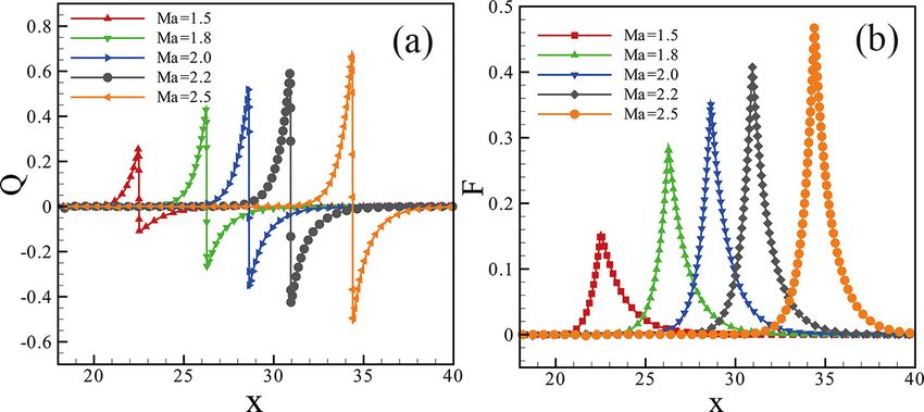
2                                                                                                        Journal Title XX(X)

Probstein 27 gave the typical structure of plasma shock          state, which allows the distribution function deviate from
front by combining two-fluid NS equations with Poisson           equilibrium state around the shock wave front. However,
equation, and the transport coefficients given by Spitzer 28     Tidman’s 36 work neglect the electron thermal conductivity,
and Braginskii 29 were adopted. The result shows an ion          which plays an important role in forming the electron
shock wave imbedded in wider electron thermal layer when         preheating layer because of the small ion-electron mass
Ma > 1.12. The thickness of ion shock is proportional to         ratio. Greenberg and Treve 38 first investigated the self-
downstream ion mean free path, and there exists a preheating     induced electric field caused by charge separation by using
layer in front of the ion shock where electron temperature is    Mott-Smith bi-Maxwellian form, but only considered the
higher than ion. Moreover, when the shock is strong (Ma =        momentum exchange between ions and electrons. Such a
10), a precursor electric shock layer appears upstream, in       treatment is insufficient because dissipative effects such
which electric effects interact with flow. Ramirez 30 studied    as ion/electron viscosity and thermal conductivity play
the nonlocal electron heat relaxation effects by generalizing    important roles in maintaining the continuity structure of
the results of Jaffrin with arbitrary ionization number Z. The   shock front. Casanova 39 computed the ionic Fokker-Planck
results prove that nonlocal electron heat transport widens       equation, combining with the electron heat equation. The
the preheating layer and smoothes the electron temperature       result shows that ionic viscosity and thermal conduction
profile. Hu 31 considered the plasma electric characters such    are much larger than classic transport coefficients assumed
as current, field and charge around the shock front. It          in hydrodynamic simulation, and the effective shock width
was found that a weak current carried by the shock could         is comparable to the width of the electronic preheating
obviously affect the shock strength. Masser 32 developed         layer, which means a hundredfold increase over the classic
semi-analytic solutions by using a two-temperature model,        value. Videl 40 then used the same model and discovered
and found the boundary between continues and discontinues        that the broaden of shock front is because of the energetic
solutions depended on the upstream Mach number. In the           ions streaming from the hot and dense plasma into the
literatures above, only one type of ion has been considered.     cold. Keenan and Simakov 41 adopted a high-fidelity Vlasov-
Simakov 33–35 then generalized the Braginskii electron fluid     Fokker-Planck code to investigate the shock structure with
description to multi-ion plasma shock waves.                     Mach number and different ion composition. By comparing
   Though much efforts and progress have been made by            the result with multi-ion hydrodynamic simulation, they find
using hydrodynamic method, such as the NS equations.             that the kinetic width of shock saturate for Ma  1, and the
It should be noted that this treatment is mainly based on        asymptotic value depends on the upstream lighter species
continuous medium hypothesis, and is valid only when             concentration.
the Knudsen number (defined as mean free path divide                It is easy to find that the study on plasma shock wave
by a characteristic length scale) Kn  1. In other words,        is facing a dilemma. From one side, the hydrodynamic
hydrodynamic method is valid only when considering               model based on NS is insufficient for describing the
behavior in a scale large enough. It is understandable           kinetic behavior of plasma. From the other side, the full
that such a treatment will be challenged when considering        kinetic model is too complicated to solve for most cases.
behavior in small scale, for example, in scale for showing       It is meaningful to develop some coarse-grained kinetic
shock structure, especially strong shock structure with          model whose physical description capability is in between
extremely high physical gradient. A more specific case is        the hydrodynamic and fully kinetic models. The Discrete
that the structure of imbedded ion shock should be explored.     Boltzmann Modeling (DBM) method is one of methods for
Moreover, the Kn of shock wave become larger as Ma               constructing such coarse-grained kinetic models 8,10 . It can
increases. The Knudsen number can also be regarded as the        be regarded as a variant hybrid of the Lattice Boltzmann
relative thermodynamic relaxation time with respect to the       Method (LBM) 42–59 and the description method of non-
time scale of flow under consideration. Since the time scale     equilibrium behavior in statistical physics. But it should be
for shocking is very small, there exist extremely strong non-    pointed out that, being different from the standard LBM in
equilibrium effects near shock front. For the convenience of     the usual sense, the DBM does not rely on the physical image
description, the non-equilibrium described by hydrodynamic       of lattice gas model where the virtual particles propagate
theory is referred to as Hydrodynamic Non-Equilibrium            from current grid to an adjacent grid in one time step.
(HNE), and the non-equilibrium described by kinetic theory       In the absence of misunderstanding, DBM is also used as
due to deviating from thermodynamic equilibrium is referred      an abbreviation for discrete Boltzmann model or discrete
to as Thermodynamic Non-Equilibrium (TNE). It is clear           Boltzmann method.
that the HNE is only one small part of TNE. Additionally,           As one of the specific applications of coarse-grained
the coefficients of viscosity and heat conduction (the two       modeling theory in non-equilibrium statistical physics in the
parameter describing the TNE) in NS are usually determined       field of fluid mechanics, the DBM is a further development
by experience or experiment.                                     of phase space description method in the form of discrete
   As a more fundamental description method, kinetic             Boltzmann equation 60 . The methodology of DBM is to
theory based on distribution function is more suitable for       decompose complex problems into parts and select a
investigating the fine structure of plasma shock. Tidman 36      perspective to study a set of kinetic properties of the
employed Boltzmann-Fokker-Planck equations by assuming           system, so it requires that the kinetic moments describing
that the distribution function of ion is a bi-Maxwellian         this set of properties maintain their values in the model
form. This form was put forward by Mott-Smith 37 . The           simplification. Based on the independent components of the
idea is that the distribution function transitions from the      kinetic moments of (f − f eq ), construct the phase space,
upstream equilibrium state to the downstream equilibrium         and the phase space and its subspaces are used to describe

Prepared using sagej.cls
Liu, Song, Xu, Zhang and Xie                                                                                                     3

the non-equilibrium behavior of the system. The research           evolves towards f eq through particle collisions, and the
perspective and modeling accuracy will be adjusted as              speed of this process is controlled by relaxation time τ .
the research progresses. With the help of DBM, kinetic             According to the different forms of f eq , the linearized
processes neglected by NS modeling, such as the non-               collision model named as Bhatnagar-Gross-Krook (BGK)
equilibrium and mutual conversion of internal energy in            model 66 , Ellipsoidal Statistical (ES) BGK model 67 , Shakov
different degrees of freedom during the reaction process,          model (for monatomic gas) 68 , Rykov model (for diatomic
etc., can be investigated 8,10–12,60–65 , where f and f eq are     gas) 69 , etc. In this work, we adopt BGK model, where f eq is
the distribution function and its corresponding equilibrium,       the Maxwellian distribution which reads
respectively.
   In order to simplify the problem and consistent with            f eq (ρ, u, T ) =
the existing literature, we focus mainly on a one-                             D/2        1/2
                                                                                                       (v − u)2     η2

                                                                          1             1
dimensional shock wave propagating in a fully ionized,             ρ                             exp −          −
                                                                        2πRT          2πnRT              2RT      2nRT
quasi-neutral, homogeneous, unmagnetized plasma with no                                                                (3)
applied external electric and magnetic fields, and the ion-
electron recombination effect are also neglected. The ion is in    where ρ, u and T are the density, bulk velocity and
single species and the charge number Zi = 1. Moreover, the         temperature, respectively. R is the gas constant. D is the
radiation effect is neglected, which means the only external       number of space dimension. η represents the extra degree
force that charge particles subjected to is electric field force   of freedom such as molecular rotation and vibration. n is the
caused by charge separation.                                       number of extra degree of freedom, according to which the
   This paper is arranged as follows. In section 2, we briefly     specific heat ratio γ could be written as,
introduce the DBM and the physical quantities used to
describe plasma shock system. In section 3, we adopt two                            γ = (D + n + 2)/(D + n)                    (4)
Riemann shock tube problems to verify the present DBM. In
section 4, we introduce the calculation parameter settings.        In the following discussion the mass of the particle (ion)
In section 5, we explore the ion peak structure and the            described by the distribution function and the gas constant R
corresponding TNE effects near the wavefront and give the          are assumed to be unity, and consequently the mass density
relationship between ion peak distribution and the intensity       equals to the number density and T is used to replace RT .
of electric force. Then, we change the magnitude of Ma and
investigate the variation trend of ion physical quantities and     Discretization of the particle velocity space
TNE effects near the peak. In section 6, we summarize and
make a conclusion for the whole paper.                             The discrete Boltzmann equation with discrete velocity vi is
                                                                   as follows,
Discrete Boltzmann modeling method                                       ∂fi       ∂fi                 1
                                                                             + viα     + Force term = − (fi − fieq )           (5)
The original Boltzmann equation reads                                    ∂t        ∂rα                 τ
              ∂f        ∂f         ∂f                              where the subscript i (= 1, ..., N ) represents the ith discrete
                   +v·      +a·        = Q(f, f )           (1)
               ∂t       ∂r         ∂v                              velocity, and the subscript α represents the x, y and z
where f is the particle distribution function. The variables t     component of space in three-dimensional case.
, v , r , a, are the time, particle velocity, space coordinate,       f (r, v, t) is defined in the (6 + 1)-dimensional phase
acceleration caused by external force, respectively. Q(f, f )      space of particle position, particle velocity and time.
is the Boltzmann collision term, which represents the change       Since particle can move towards any direction range
of distribution function f caused by particle collisions.          from (−∞, +∞), the conventional discrete method for
From Boltzmann equation to discrete Boltzmann model, two           discretizing time and space is not suitable for the
steps of coarse-grained physical modeling are required. The        discretization of particle velocity space. Therefore, the
principle of coarse-grained modeling is that the physical          discrete distribution function fi do not have specific physical
quantities we concern must keep the same values before and         meaning, also do not correspond to the probability that
after simplification.                                              particle velocity equal to vi . What we used to analyzing
                                                                   the system is not the specific value of fi , but the kinetic
Linearization of the collision term                                moments. So the principle is that integral form of the kinetic
Compared with Liouville equation, Boltzmann equation is            moments is equal to the sum form, as follows,
a much coarse-grained model. However, the collision term                             Z               X
Q(f, f ) in the right-hand of Eq. (1) is still too complicated                         f Ψ(v)dv =         fi Ψ(vi )             (6)
to solve for most practical problems. A common practice                                               i
is to substitute the collision term with a linearized collision
operator, and write the Boltzmann equation as the following        where Ψ(v) = [1, v, vv, · · · ] correspond to different kinetic
form,                                                              moments. It is easy to find that the dimension of fi equals
                                                                   to that of f v. According to Chapman-Enskog multi-scale
          ∂f      ∂f       ∂f       1                              analysis, Eq. (6) can be finally expressed as
             +v·      +a·       = − (f − f eq )        (2)
          ∂t      ∂r       ∂v       τ                                            Z
where f eq is the local particle equilibrium distribution
                                                                                                     X eq
                                                                                    f eq Ψ0 (v)dv =      fi Ψ0 (vi )           (7)
function. The physical meaning of this practice is that f                                             i

Prepared using sagej.cls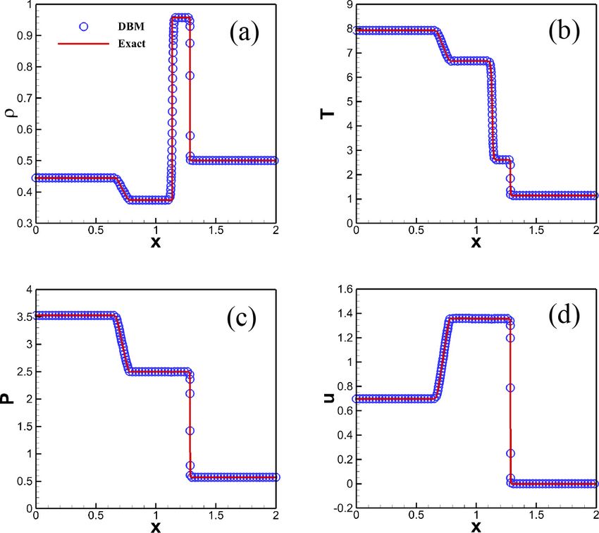
4 Journal Title XX(X)
where Ψ0 (v) corresponds to higher order kinetic moments. forcing term, where e is the charge of proton. When the non-
A key step for the DBM simulation is the calculation of fieq equilibrium effects caused by f deviating from f eq in force
on the right hand of Eq. (5). term is not significant, we have
The modeling precision of DBM can be adjusted
according to the practical needs. As the first attempt for ∂f ∂f eq (v − u) eq
a· ≈a· = −eE · f . (15)
constructing DBM for plasma, in this paper we consider ∂v ∂v T
the case where the system deviates from its thermodynamic
Consequently, the DBM evolution equation (5) becomes
equilibrium slightly and consequently only the first order
TNE effects are needed to be taken into account. ∂fi ∂fi (v − u) eq 1
To construct such a DBM, the values of seven kinetic + viα − eE · fi = − (fi − fieq ).
∂t ∂rα T τ
moments shown in the left hand side of Eqs. (8)-(14), should (16)
keep unchanged when being calculated in the following It is easy to find that the following hydrodynamic model,
summation form,
∂ρ
+ ∇ · (ρu) = 0,
Z Z X eq
f eq dvdη = ρ =
fi , (8)
∂t
∂ρu
+ ∇ · (ρuu) + ∇p = −∇ · P 0 + ρeE,
∂t
∂ET + ∇ · [(E + p)u] = ∇ · [κ∇T + P 0 · u] + ρeE · u,
Z Z X
f eq vdvdη = ρu = fieq v,
(9) T
∂t
(17)
Z Z is one part of the current DBM, where p = ρT is the
1 pressure, ET = ρeint + (ρu2 )/2 is the system energy per
f eq v 2 + η 2 dvdη = ET
(10)
2 unit volume, and eint = (n + 2)T /2 is the internal energy.
u2
X
(D + n) T 1 µ = τ p and κ = cp τ p are the coefficients of viscosity and
fieq vi2 + ηi2 ,
=ρ + = thermal conductivity, respectively.
2 2 2
In addition to the HNE behavior, DBM could simultane-
Z Z X ously give the the most relevant TNE effects accompanying
f eq vvdvdη = pI + ρuu = fieq vi vi , (11) with the macroscopic flows. In other words, DBM can
be regarded as a hydrodynamic model supplemented by
a coarse-grained model of the most relevant TNE effects.
The way to obtain TNE quantities is by comparing the
Z Z
1 2
f eq
v + η 2 vdvdη = (ET + p) u = ρu
(12) distribution function f to the local equilibrium distribution
2
(D + n + 2) T u2
X
1 function f eq with kinetic moments at a certain time, which
fieq vi2 + ηi2 vi ,
+ = defined as,
2 2 2
∆m = Mm (f ) − Mm (f eq ), (18)
Z Z
f eq vvvdvdη = p(uα eβ eγ δβγ + eα uβ eγ (13) ∆∗m = Mm
∗ ∗
(f ) − Mm (f eq ), (19)
X eq
δαγ + eα eβ uγ δαβ ) + ρuuu = fi vi vi vi , where Mm represent the different orders of non-central
∗
kinetic moments involving bulk velocity, and Mm represents
Z Z the different orders of central kinetic moments describing the
1 2 thermal fluctuation information. Of all the kinetic moments,
f eq v + η 2 vvdvdη = T (ET + p) I
(14)
2 the first three will always be equal when displace f eq
u2
(D + n + 2) T with f , which is determined by the conservation law of
+ uu (ET + 2p) = p +
2 2 mass, momentum and energy. However, the result will be
(D + n + 4) T u2
different for higher order moments, and each of these non-
I + ρuu + = equilibrium quantities reflects the extent system deviated
2 2
X eq 1 from local thermodynamic equilibrium from one aspect. The
vi2 + ηi2 vi vi ,
fi non-equilibrium quantities used in this paper are defined as
2 follows,
where ηi is the discrete correspondence of η. The DBM for X X eq
higher order TNE flows can be constructed in a similar way
∆2 = fi vi vi − fi vi vi ,
via considering higher order TNE effects (i.e. more kinetic X X eq
f v2 + η2 v − v2 + η2 v ,
∆ =
3,1 i i i i fi i i i
moments have to be considered).
X X
In this work, we consider only one type of ion with
∆3 = fi vi vi vi − fieq vi vi vi ,
charge Zi = 1. The electron is assumed to be inertialess and
X X eq
fi vi2 + ηi2 vi vi − fi vi2 + ηi2 vi vi ,
∆4,2 =
always in thermodynamic equilibrium. The behavior of ion
is described by the distribution function f which follows (20)
Eq. (5). The only interaction taken into account between By substituting vi in Eq. (20) with (vi − u), a TNE quantity
ion and electron is the electric field force caused by charge ∆∗m based on the central kinetic moments can also be
separation. The electric field force a = eE is added into the obtained.
Prepared using sagej.cls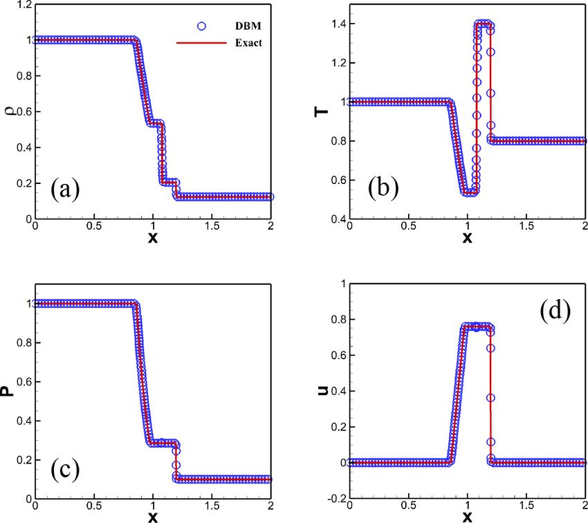
Liu, Song, Xu, Zhang and Xie 5
of discrete velocities are shown in Eq. (26),
(i − 1)π (i − 1)π
v1 cos , sin , i=1−4
2 2
√
(2i − 1)π (2i − 1)π
2v2 cos , sin , i=5−8
4 4
vi =
√
(2i − 9)π (2i − 9)π
2v3 cos , sin , i = 9 − 12
4 4
(i − 13)π (i − 13)π
v4 cos , sin , i = 13 − 16
2 2
(26)
and ηi = η0 for i = 5, 6, 7, 8, else ηi = 0.
Validation and verification
Figure 1. Schematic of the discrete velocity model.
In this section, we choose two typical one-dimensional
Riemann problems to confirm the validity of the present
model for capturing main structures in flow. And the spatial
In this work we consider a one-dimensional shock, so the
and temporal derivatives are discretized by using forward
electric field force is only in x direction. Thus, we get the
Euler finite difference scheme and the nonoscillatory nonfree
following evolution equation,
dissipative (NND) scheme, respectively.
∂fi ∂fi eEx (vix − ux ) eq 1 Sod shock tube problem
+ viα − fi = − (fi − fieq ).
∂t ∂rα T τ
(21) The initial conditions are as follows,
The Poisson equation gives (
(ρ, T, u, v)L = (1.0, 1.0, 0.0, 0.0), x≤1
(27)
d2 ϕ e (ni − ne ) (ρ, T, u, v)R = (0.125, 0.8, 0.0, 0.0), x>1
=− (22)
dx2 ε0 where the subscript “L” and “R” represent the left and
right sides of the discontinuity interface. The grid number
where ϕ is the space potential, ni is the ion number density of calculated region is [Nx × Ny ] = [2000 × 1], and the
which is equals to ρi and ne is the electron number density. initial interface is located at x = 1. The meshing size is
ε0 is the vacuum permittivity. The electron is assumed to ∆x = ∆y = 1 × 10⁻³ , and the time step is ∆t = 1 × 10⁻⁵ .
be always in thermodynamic equilibrium, so the electron Parameters for discrete velocities are v1 = 0.5, v2 = 1.0,
density obeys Boltzmann distribution as v3 = 2.9, and v4 = 4.5. The parameter for extra degree
is η0 = 5. The other parameters are τ = 2 × 10⁻⁵ , n =
eϕ 0 (i.e., γ = 2). In the y direction, the periodic boundary is
ne = ne0 exp (23)
kTe adopted. In the x direction, the left and right boundary are
assumed always in the initial equilibrium state, which are
Where ne0 is the initial electron density when ϕ is equal ( eq
to zero. k = R/NA is the Boltzmann constant, and is equal fi,−1,t = fi,0,t = fi,1,t=0
eq (28)
to 1 for particle mass NA and gas constant R are unity. By fi,Nx +2,t = fi,Nx +1,t = fi,N x ,t=0
substituting Eq. (22) with Eq. (23) and assuming the vacuum
permittivity ε0 is unity, the Poisson equation reads where the subscripts “−1”, “0”, “Nx + 1” and “Nx + 2”
represent the ghost nodes on the left and right sides. Figure
d2 ϕ
eϕ
2 shows the comparison between the analytical result of
= ene0 exp − eni (24) sod shock tube problem and the result of DBM at t = 0.1.
dx2 Te
Obviously, the result of DBM is in good agreement with
the exact solution. Here the exact solution is in Euler level,
The proton charge e, electron temperature Te , and initial which means the dissipation effects such as viscosity and
electron density ne0 are assumed to be unity. Then the thermal conduction have been ignored.
Poisson reads
d2 ϕ Lax shock tube problem
= exp (ϕ) − ni (25)
dx2 The initial conditions are as follows,
(
In this work, we consider only the two dimensional case. (ρ, T, u, v)L = (0.445, 7.928, 0.698, 0.0), x≤1
(29)
The seven kinetic moment relations, (8)-(14), have sixteen (ρ, T, u, v)R = (0.5, 1.142, 0.0, 0.0), x>1
components in two-dimensional case, so at least sixteen
discrete velocities are needed. The sketch map of discrete Figure 3 shows the computation result of density, pressure,
velocity model we adopted is shown in Figure. 1. The values temperature and velocity in x direction at t = 0.1, where the
Prepared using sagej.cls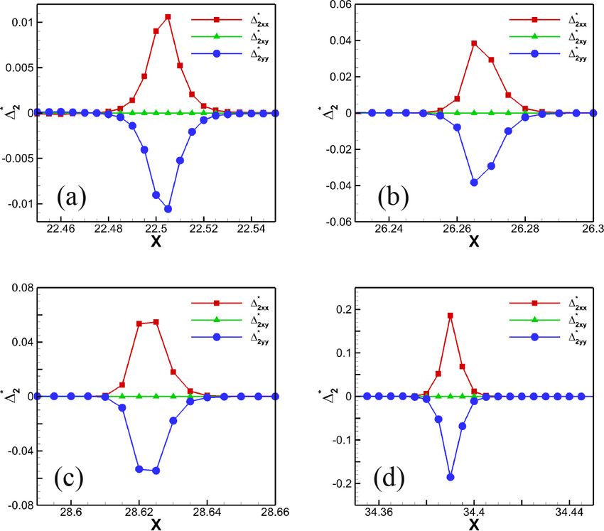
6 Journal Title XX(X)
Calculation parameter settings
In the simulation of plasma shock wave, the initial
macroscopic quantities are arranged as follows,
(
(ρ, u1 , u2 , T )L = (ρ0 , u0 , 0, T0 ), x ≤ Nx /8
(30)
(ρ, u1 , u2 , T )R = (1.0, 0.0, 0.0, 1.0), x > Nx /8
where the subscripts “L” and “R” indicates the downstream
and upstream of shock wave. ρ0 , u0 , T0 are the initial
downstream density, bulk velocity, temperature, respectively.
The initial upstream and downstream macroscopic quantities
are connected by the Rankine-Hugoniot relations, which
can be deduced from Eq. (17) after several steps. First, by
substituting Eq. (17) with Eq. (25) we get the following
equations
∂ρ
+ ∇ · (ρu) = 0,
Figure 2. Comparison between Riemann solutions and DBM
∂t
∂ρu
results of Sod shock tube problem. (a) density, (b) pressure, (c)
+ ∇ · (ρuu) + ∇p = ∇2 ϕ − exp(ϕ) ∇ϕ, (31)
temperature, (d) horizontal velocity. ∂t
∂E
T + ∇ · [(E + p)u] = −ρu∇ϕ,
T
∂t
After simplification, Eq. (31) becomes
∂ρ
+ ∇ · (ρu) = 0,
∂t
2
∂ρu [∇ϕ] (32)
+ ∇ · [ρuu + p − + exp(ϕ)] = 0,
∂t 2
∂ET + ϕ ∂ρ + ∇ · [(ET + p + ρϕ)u] = 0,
∂t ∂t
For the steady state, Eq. (32) becomes
∇ · (ρu) = 0,
2
(∇ϕ) (33)
∇ · [ρuu + p − + exp(ϕ)] = 0,
2
∇ · [(ET + p + ρϕ)u] = 0,
For the steady state upstream and downstream flow, there
Figure 3. Comparison between Riemann solutions and DBM exist no electric current and charge separation, which means
results of Lax shock tube problem. (a) density, (b) pressure, (c) ∇ϕ equals to zero. Then the Rankine-Hugoniot relations
temperature, (d) horizontal velocity.
ρ1 u1 = ρ2 u2
ρ1 u1 u1 + ρ1 T1 + exp(ϕ1 ) = ρ2 u2 u2 + ρ2 T2 + exp(ϕ2 )
blue circles indicate the DBM results and the red solid lines
γ u2 γ u2
T1 + 1 + ϕ1 = T2 + 2 + ϕ2
indicate the exact Riemann solution in Euler level. The grid γ−1 2 γ−1 2
number of calculated region is [Nx × Ny ] = [2000 × 1], and (34)
the initial interface is also located at x = 1. The parameter are deduced, where “1” and “2” represent the upstream and
are set to be ∆x = ∆y = 1 × 10⁻³ , ∆t = 1 × 10⁻⁵ , τ = downstream. Also, the Poisson equation becomes
2 × 10⁻⁵ , η0 = 5, n = 0 (i.e., γ = 2), and v1 = 0.5, v2 =
ρi = ni = exp(ϕ) (35)
1.0, v3 = 2.9, v4 = 4.5. The boundary conditions in x and
y direction are consistent with the setting in sod shock tube After setting the initial conditions, the the Poisson equation
problem. From Figure. 3, we can observe that the two results is calculated for the whole computational domain with time
are in good agreement with each other. evolution. The accurate solution of Poisson is assumed as
From the results of two one-dimensional Riemann follows
problems, we find that the present DBM with appropriate ϕ = ϕ0 + δϕ (36)
discretization schemes can capture the main structure of flow By inserting Eq. (36) into Eq. (25), the Poisson equation
with shock wave, expanding wave and contact discontinuity reads
effectively, which is a basic capability for simulating shock
wave propagating in plasma. ∂ 2 x (ϕ0 ) + ∂ 2 x (δϕ) − exp(ϕ0 + δϕ) + ni = 0 (37)
Prepared using sagej.cls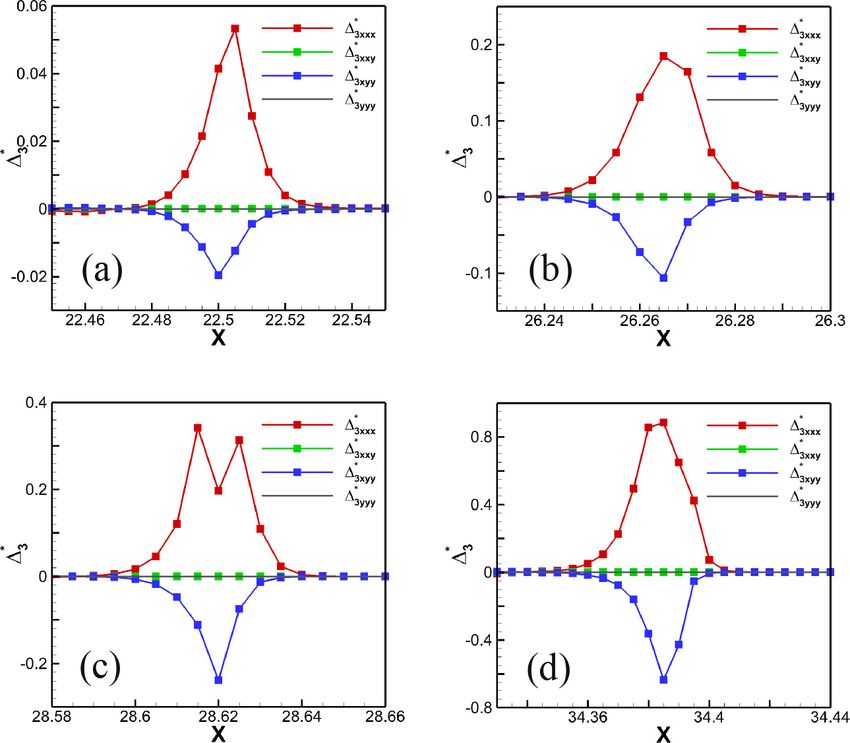
Liu, Song, Xu, Zhang and Xie                                                                                                      7

Figure 4. Density, temperature, pressure and horizonal velocity   Figure 7. Quantity of charge and electric field force varies with
distribution when Ma = 1.5. (a) plasma shock wave at t = 8,       Ma at t = 8. (a) charge, (b) electric field force.
(b) shock wave in neutral fluids at t = 2.

                                                                  direction, around plasma and neutral fluid shock when Ma =
                                                                  1.5 and Ma = 1.8, respectively. It is found that the plasma
                                                                  shock wave is very different from the shock wave in neutral
                                                                  fluids, and somewhat similar to the detonation wave. The
                                                                  macroscopic quantities both exhibit spike structures and
                                                                  reach the maximum value in the same position, but the
                                                                  maximum value of these macroscopic quantities are all less
                                                                  than the corresponding downstream value of shock wave in
                                                                  neutral fluids. Besides, the result is also different comparing
Figure 5. Density, temperature, pressure and horizonal velocity   with previous studies for not only temperature but also
distribution when Ma = 1.8. (a) plasma shock wave at t = 8,       density, velocity and pressure appear maximum value that
(b) shock wave in neutral fluids at t = 2.                        exceeds the downstream equilibrium value. The reason is that
                                                                  the exchange of momentum and energy between electrons
                                                                  and ions are ignored in our hypothesis.
                                                                     Figure 6 describes the electrical quantities, including
                                                                  electric field force, potential and net charge distribution
                                                                  in x direction, around plasma when Ma = 1.5 and Ma =
                                                                  1.8, respectively. It is observed that the electric field force
                                                                  also behave as a spike, but the net charge presenting as
                                                                  two opposite spikes. Through further analysis of data, it
                                                                  is found that the peak position of electric field force does
                                                                  not coincide with macroscopic quantities, but locate at the
Figure 6. Electric field force, potential and net charge          position where the net charge Q = 0. The peak position of
distribution of plasma shock wave at t = 8. (a) Ma = 1.5, (b)
                                                                  positive net charge is coincide with macroscopic quantities,
Ma = 1.8.
                                                                  but the peak position of negative net charge is locate at
                                                                  upstream. Intuitively, the net charge represents the extent of
It is further assumed that                                        charge separation. Because the proton charge e is assume
                                                                  to unity, the net charge is also equal to net density, so
                   ∂ 2 x (ϕ0 ) − exp(ϕ0 ) + ni = f0        (38)   there occurs charge separation or density difference during
                                                                  the motion of plasma shock wave and forms the ion
Thus the Poisson equation reads,                                  and electron concentration region in the downstream and
                                                                  upstream, respectively. In terms of the net charge spikes
                    ∂ 2 x (δϕ) − exp(ϕ0 )δϕ = −f0          (39)
                                                                  amplitude and width, it is observed that the absolute value
Eq. (39) is a tridiagonal matrix, so the chase method is          of positive net charge peak is greater than that of negative
used for calculation. The grid number of calculated region is     net charge peak, but the negative net charge region is wider
[Nx × Ny ] = [10000 × 1], and the initial interface is located    than positive net charge region, which is determined by the
at Nx /8. The simulation conditions are ∆x = ∆y = 5 ×             fact that the total charge of plasma is zero. The distribution
10−3 , ∆t = 1 × 10⁻⁴ , τ = 2 × 10⁻⁴ , n = 0 (i.e., γ = 2).        of net charge also demonstrate that the electron tends to
In order to maintain the stability of model, we choose v1 =       move towards upstream and the ion tends to move towards
0.5, v2 = 1.0, v3 = 2.9, v4 = 4.5, and η0 = 5.                    downstream, and the diffusion area of electron is longer than
                                                                  ion because of the small electron/ion mass ratio.
Result and disscussion
                                                                  Macroscopic and electrical quantities around
Macroscopic quantities around plasma shock                        plasma shock wave
wave                                                              We then investigate the variations of macroscopic and
We first investigate the steady state structure of plasma         electrical quantities with Ma number. Figure 7 shows the net
shock wave. Figures 4 and 5 give the macroscopic quantities,      charge and electric field force distribution around the shock
including density, pressure, temperature and velocity in x        front for the cases of Ma = 1.5, 1.8, 2.0, 2.2, 2.5. It is found

Prepared using sagej.cls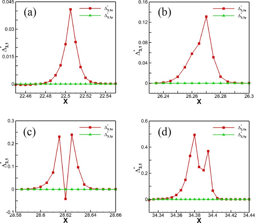
8 Journal Title XX(X)
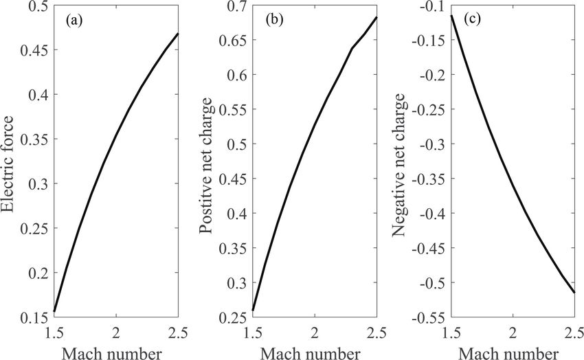
Figure 10. Electrical quantities peak value varies with Ma. (a)
electric force, (b) positive net charge, (c) negative net charge.
Figure 8. Macroscopic quantities peak value varies with Ma.
(a) density, (b) temperature, (c) pressure, (d) horizontal velocity.
Figure 11. Non-equilibrium quantities versus x when
Ma = 1.8. (a) ∆∗2 , (b) ∆∗3,1 , (c) ∆∗3 , (d) ∆∗4,2 .
downstream values with increasing Ma. It is observed that
Figure 9. Difference value between macroscopic quantities the difference of density first increases, then decreases with
peak value and downstream value varies with Ma. (a) density, Ma. The differences of temperature and pressure increase
(b) temperature, (c) pressure, (d) horizontal velocity. with Ma. The difference of velocity decreases linearly with
Ma. From Figures. 9 (b) and (c), it is also observed that the
growth rates of both decrease gradually with the increase of
that an electric double layer appeared around the shock front. Ma, and the growth rate of temperature decreases faster.
The large inertia of the ions causes them to lag behind, so the Figure 10 shows the electrical quantity peak values versus
wave front charge is negative and the wave rear charge is Ma. It can be seen from Figure. 10 (a) that the electric
positive. The peak value on the left side is larger than that field force remains growing as Ma increases, indicating that
on the right side, and the width on the left is smaller than the the extent of charge separation increases. The electric field
right, which means the left side is much steeper than the right force is the expression of the non-uniform charge distribution
side. As the Mach number increase, the two peaks of both inside the shock wave, so there exists strong charge non-
two sides increase, indicating that electrons tend to move uniform phenomenon inside the shock wave, which greatly
upstream of the shock wave with the increasing of Ma. This affects the shock wave structure. From Figures. (b) and (c),
movement tendency makes the degree of charge separation it is observed that the absolute values of the positive and
increase, and the electric field force also becomes larger. negative peak keep growing, but the growth rates of both
Figure 8 shows the peak values of macroscopic quantities keep decreasing gradually.
varies with Ma. Obviously, the four peak values increases
with Ma approximately in linear form. However, the growth
rate of temperature and pressure increase slowly with Ma,
Non-equilibrium Effects around plasma shock
and the growth rate of density and horizontal velocity wave
decrease slowly with Ma. Figure 11 shows the non-equilibrium quantities of ion when
Figure 9 gives the evolution of differences between Ma=1.8. Among the different types of TNE defined by Eq.
macroscopic quantity peak values and the corresponding (19), the most commonly used are non-organized momentum
Prepared using sagej.cls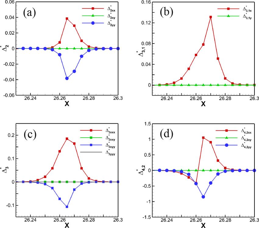
Liu, Song, Xu, Zhang and Xie 9
Figure 12. ∆∗2 varies with Ma. (a) Ma=1.5, (b) Ma=1.8, (c)
Figure 13. ∆∗3,1 varies with Ma. (a) Ma=1.5, (b) Ma=1.8, (c)
Ma=2.0, (d) Ma=2.5.
Ma=2.0, (d) Ma=2.5.
flux (NOMF) ∆∗2 and non-organized energy flux (NOEF)
∆∗3,1 . The former have three components including ∆∗2xx ,
∆∗2xy and ∆∗2yy . ∆∗2xx and ∆∗2yy indicate the momentum
flux in x and y direction, respectively. While ∆∗2xy indicates
the shear effect. ∆∗3,1 represents the energy flux, and its two
components ∆∗3,1x and ∆∗3,1y indicate the energy flux in x
and y direction, respectively. From Figure. 11 (a) it could
be found that the NOMF was symmetrically distributed
in the x and y directions, which means the way system
deviate from equilibrium in x and y direction is similar but
towards different direction. It should be note that, the way
system deviate from equilibrium in three-dimensional case
can also be inferred from two-dimensional results. Due to the
symmetry of the system, we cannot assume that the way the
system deviates from equilibrium in the y and z directions
are different, so the ∆∗2xx is the same for two and three
dimensional case. However, ∆∗2yy will be evenly distributed
in the y and z directions for three-dimensional case, and the Figure 14. ∆∗3 varies with Ma. (a) Ma=1.5, (b) Ma=1.8, (c)
sum of these three components is zero. Besides, ∆∗2xy is zero, Ma=2.0, (d) Ma=2.5.
indicating that there is no shear effect. Figure 11 (c) gives the
distribution of ∆∗3,1 . It is observed that ∆∗3,1x always deviate
from equilibrium in one direction, and reaches its maximum
at the wave front. ∆∗3,1y is zero, which means there exist no
non-equilibrium effect of energy flux in y direction. ∆∗3 and
∆∗4,2 are correspond to flux of viscous effect and heat flux.
From Figure. 11 (b), it is observed that the flux of ∆∗2xx
and ∆∗2yy in x direction is not zero, and both deviate from
equilibrium toward one direction. However, the magnitude
of ∆∗3xxx is larger than ∆3xyy . Figure 11 (d) describes the
flux of ∆∗3,1 . It is found that the flux of ∆∗3,1x in x direction
appears a reverse at downstream, but the flux of ∆∗3,1y in y
direction always toward one direction.
By changing the magnitude of the Mach number, we
further investigate the variation of the non-equilibrium
effects with Mach number. Some simulation results are
shown in Figures. 12 - 15 which are for ∆∗2 , ∆∗3,1 , ∆∗3
and ∆∗4,2 , respectively. Firstly, the amplitudes of all the
four quantities increase with Ma. Then, from Figure. 13,
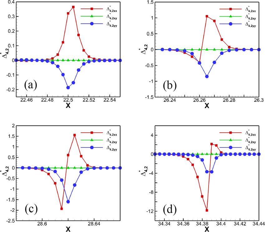
Figure 15. ∆∗4,2 varies with Ma. (a) Ma=1.5, (b) Ma=1.8, (c)
it is observed that the NOEF in x direction ∆∗3,1x appears Ma=2.0, (d) Ma=2.5.
a reverse when Ma = 2.0. When Ma = 2.5, ∆∗3,1x become
Prepared using sagej.cls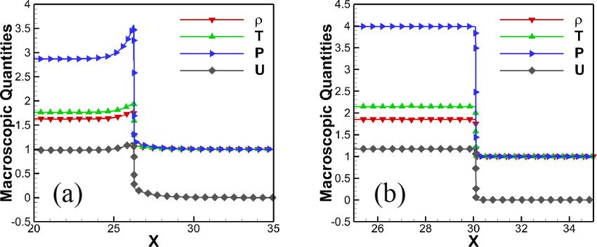
10                                                                                                              Journal Title XX(X)

positive again, forming a bimodal structure, which means           (Beijing Institute of Technology) (under Grant No. KFJJ21-16M),
the increasing Ma causes the strong non-equilibrium of             and the China Postdoctoral Science Foundation (under Grant No.
energy flux in x direction. Finally, an evident difference from    2019M662521).
the case of detonation wave 15 is that ∆∗4,2 is qualitatively
different from ∆∗2 for the plasma shock wave.

                                                                   References
Conclusion
                                                                    1. Craxton R, Anderson K, Boehly T et al. Direct-drive inertial
A discrete Boltzmann model for plasma shock wave is
                                                                       confinement fusion: A review. Physics of Plasmas 2015;
constructed. The model works for both steady and un-
                                                                       22(11): 110501.
steady shock waves. The electron is assumed inertialess
                                                                    2. Betti R and Hurricane O. Inertial-confinement fusion with
and always in thermodynamic equilibrium. The Rankine-
                                                                       lasers. Nature Physics 2016; 12(5): 435–448.
Hugoniot relations for single fluid theory of plasma shock
                                                                    3. Zhou Y. Rayleigh–taylor and richtmyer–meshkov instability
wave is derived. It is found that the physical structure of
                                                                       induced flow, turbulence, and mixing. i. Physics Reports 2017;
shock wave in plasma is significantly different from that in
                                                                       720: 1–136.
neutral fluid and somewhat similar to that of detonation wave
                                                                    4. Zhou Y. Rayleigh–taylor and richtmyer–meshkov instability
from the sense that a peak appears in the front. The charge
                                                                       induced flow, turbulence, and mixing. ii. Physics Reports 2017;
of electricity deviates oppositely from neutrality in upstream
                                                                       723: 1–160.
and downstream of the shock wave. The large inertia of the
                                                                    5. Wang Z, Xue K and Han P. Bell–plesset effects on rayleigh–
ions causes them to lag behind, so the wave front charge
                                                                       taylor instability at cylindrically divergent interfaces between
is negative and the wave rear charge is positive. The non-
                                                                       viscous fluids. Physics of Fluids 2021; 33(3): 034118.
equilibrium effects around the shock front become stronger
                                                                    6. Xue K, Shi X, Zeng J et al. Explosion-driven interfacial
with increasing Mach number. The variations of HNE and
                                                                       instabilities of granular media. Physics of Fluids 2020; 32(8):
TNE with Mach number are numerically investigated. The
                                                                       084104.
characteristics of TNE can be used to distinguish plasma
                                                                    7. Pham-Van-Diep G, Erwin D and Muntz E. Nonequilibrium
shock wave from detonation wave.
                                                                       molecular motion in a hypersonic shock wave. Science 1989;
   It is understandable that the dissipative effects of electron       245(4918): 624–626.
and the diffusion effects between ion and electron have             8. Xu A, Zhang G and Ying Y. Progess of discrete boltzmann
not been taken into account in this work. It is still an               modeling and simulation of combustion system (in chinese).
open topic that DBM for more practical cases where both                Acta Physica Sinica 2015; 64(4): 184701.
the electron thermal conductivity and momentum/energy               9. Liu H, Kang W, Duan HL et al. Recent progresses on numerical
transfer between ion and electron are important. The two               investigations of microscopic structure of strong shock waves
fluid DBM for plasma is in progress, which will be published           in fluid (in chinese). Scientia Sinica (Physica, Mechanica &
in future.                                                             Astronomica) 2017; 47(7): 19–27.
   Finally, it should be noted that, like the NS model,            10. Xu A, Zhang G and Zhang Y. Discrete boltzmann modeling
DBM is a theoretical model to describe the behavior of                 of compressible flows. In Kyzas GZ and Mitropoulos AC
the coarse-grained system, and the scope and depth of its              (eds.) Kinetic Theory, chapter 02. Rijeka: InTech, 2018. DOI:
description of the dynamic properties of the system can                10.5772/intechopen.70748. URL http://dx.doi.org/
be adjusted according to the research needs of specific                10.5772/intechopen.70748.
problems.The DBM is the same as the NS model, and it               11. Xu A, Chen J, Song J et al. Progress of discrete boltzmann
is necessary to select the appropriate numerical calculation           study on multiphase complex flows (in chinese).             Acta
method before the numerical experiment is carried out.                 Aerodynamica Sinica 2021; 39(3): 138–169. DOI:10.7638/
From the point of view of the research needs of physical               kqdlxxb-2021.0021.
problems, we can choose any numerical calculation method           12. Xu A, Shan Y, Chen F et al. Progress of mesoscale modeling
that meets the research needs of physical problems and is              and investigation of combustion multiphase flow (in chinese).
allowed by the current hardware and software environment.              Acta Aeronautica et Astronautica Sinica 2021; 42(12): 625842.
Readers interested in numerical methods may refer to more              DOI:10.7527/S10006893.2021.25842.
specialized literature.                                            13. Liu H, Kang W, Zhang Q et al.               Molecular dynamics
                                                                       simulations of microscopic structure of ultra strong shock
Acknowledgements                                                       waves in dense helium. Frontiers of Physics 2016; 11(6): 1–
   The authors thank Lifeng Wang, Hongbo Cai, Yingkui Zhao             11.
for helpful discussions on plasma and implosion physics, thank     14. Liu H, Zhang Y, Kang W et al. Molecular dynamics simulation
Yanbiao Gan, Feng Chen, Chuandong Lin, Ge Zhang, Guanglan              of strong shock waves propagating in dense deuterium, taking
Sun, Jie Chen, Dejia Zhang, Yiming Shan, Hanwei Li, and Cheng          into consideration effects of excited electrons. Physical Review
Chen for helpful discussions on DBM, thank Long Miao, Song             E 2017; 95(2): 023201.
Bai, Dongfeng Yan, Xiaolong Yi and Fuwen Liang for helpful         15. Yan B, Xu AG, Zhang GC et al. Lattice boltzmann model for
discussions on the article organization. This work was supported       combustion and detonation. Frontiers of Physics 2013; 8(1):
by the National Natural Science Foundation of China (under             94–110.
Grant Nos. 11772064, 12172061, 12102397 and 11602162), CAEP        16. Chuan-Dong L, Ai-Guo X, Guang-Cai Z et al. Polar coordinate
Foundation (under Grant No. CX2019033), the opening project            lattice boltzmann kinetic modeling of detonation phenomena.
of State Key Laboratory of Explosion Science and Technology            Communications in Theoretical Physics 2014; 62(5): 737.

Prepared using sagej.cls
Liu, Song, Xu, Zhang and Xie 11
17. Lin C, Xu A, Zhang G et al. Polar-coordinate lattice boltzmann 38. Greenberg O and Treve Y. Shock wave and solitary wave
modeling of compressible flows. Physical Review E 2014; structure in a plasma. The Physics of Fluids 1960; 3(5): 769–
89(1): 013307. 785.
18. Lin C, Xu A, Zhang G et al. Double-distribution-function 39. Casanova M, Larroche O and Matte JP. Kinetic simulation of
discrete boltzmann model for combustion. Combustion and a collisional shock wave in a plasma. Physical Review Letters
Flame 2016; 164: 137–151. 1991; 67(16): 2143.
19. Zhang Y, Xu A, Zhang G et al. Kinetic modeling of detonation 40. Vidal F, Matte J, Casanova M et al. Ion kinetic simulations
and effects of negative temperature coefficient. Combustion of the formation and propagation of a planar collisional shock
and Flame 2016; 173: 483–492. wave in a plasma. Physics of Fluids B: Plasma Physics 1993;
20. Gan Y, Xu A, Zhang G et al. Discrete boltzmann trans-scale 5(9): 3182–3190.
modeling of high-speed compressible flows. Physical Review 41. Keenan BD, Simakov AN, Chacón L et al. Deciphering the
E 2018; 97(5): 053312. kinetic structure of multi-ion plasma shocks. Physical Review
21. Xu AG, Zhang GC, Zhang YD et al. Discrete boltzmann E 2017; 96(5): 053203.
model for implosion-and explosionrelated compressible flow 42. Succi S. The lattice Boltzmann equation: for fluid dynamics
with spherical symmetry. Frontiers of Physics 2018; 13(5): 1– and beyond. Oxford university press, 2001.
14. 43. Shan X and Chen H. Lattice boltzmann model for simulating
22. Zhang YD, Xu AG, Zhang GC et al. Discrete ellipsoidal flows with multiple phases and components. Physical review E
statistical bgk model and burnett equations. Frontiers of 1993; 47(3): 1815.
Physics 2018; 13(3): 1–13. 44. Zhang Y, Qin R and Emerson DR. Lattice boltzmann
23. Zhang Y, Xu A, Zhang G et al. Discrete boltzmann method for simulation of rarefied gas flows in microchannels. Physical
non-equilibrium flows: Based on shakhov model. Computer review E 2005; 71(4): 047702.
Physics Communications 2019; 238: 50–65. 45. Ambrus VE and Sofonea V. Quadrature-based lattice
24. Lin C, Luo KH, Xu A et al. Multiple-relaxation-time boltzmann models for rarefied gas flow. Flowing Matter 2019;
discrete boltzmann modeling of multicomponent mixture with : 271.
nonequilibrium effects. Physical Review E 2021; 103(1): 46. Chen F, Xu A, Zhang G et al. Multiple-relaxation-time
013305. lattice boltzmann approach to compressible flows with flexible
25. Qiu R, Bao Y, Zhou T et al. Study of regular reflection specific-heat ratio and prandtl number. EPL (Europhysics
shock waves using a mesoscopic kinetic approach: Curvature Letters) 2010; 90(5): 54003.
pattern and effects of viscosity. Physics of Fluids 2020; 32(10): 47. Li Q, Luo K, Gao Y et al. Additional interfacial force in
106106. lattice boltzmann models for incompressible multiphase flows.
26. Jukes J. The structure of a shock wave in a fully ionized gas. Physical Review E 2012; 85(2): 026704.
Journal of Fluid Mechanics 1957; 3(3): 275–285. 48. Wang Z, Wei Y and Qian Y. A simple direct heating
27. Jaffrin MY and Probstein RF. Structure of a plasma shock thermal immersed boundary-lattice boltzmann method for its
wave. Physics of Fluids 1964; 7(10): 1658–1674. application in incompressible flow. Computers & Mathematics
28. Spitzer L. Physics of fully ionized gases. Interscience with Applications 2020; 80(6): 1633–1649.
publishers Inc., New York, 1956. 49. Chen Z, Shu C and Tan D. Highly accurate simplified lattice
29. Braginskii S and Leontovich M. Reviews of plasma physics, boltzmann method. Physics of Fluids 2018; 30(10): 103605.
1965. 50. Wang Y, Zhong C, Cao J et al. A simplified finite volume
30. Ramirez J, Sanmartin J and Fernández-Feria R. Nonlocal lattice boltzmann method for simulations of fluid flows from
electron heat relaxation in a plasma shock at arbitrary laminar to turbulent regime, part i: Numerical framework and
ionization number. Physics of Fluids B: Plasma Physics 1993; its application to laminar flow simulation. Computers &
5(5): 1485–1490. Mathematics with Applications 2020; 79(5): 1590–1618.
31. Hu Y and Hu X. The properties and structure of a plasma non- 51. Saadat MH, Bösch F and Karlin IV. Semi-lagrangian lattice
neutral shock. Physics of Plasmas 2003; 10(7): 2704–2711. boltzmann model for compressible flows on unstructured
32. Masser T, Wohlbier J and Lowrie R. Shock wave structure for meshes. Physical Review E 2020; 101(2): 023311.
a fully ionized plasma. Shock waves 2011; 21(4): 367–381. 52. Fei L, Du J, Luo K et al. Modeling realistic multiphase
33. Simakov AN and Molvig K. Electron transport in a collisional flows using a non-orthogonal multiple-relaxation-time lattice
plasma with multiple ion species. Physics of Plasmas 2014; boltzmann method. Physics of Fluids 2019; 31(4): 042105.
21(2): 024503. 53. Qiu R, Bao Y, Zhou T et al. Study of regular reflection
34. Simakov AN and Molvig K. Hydrodynamic description of shock waves using a mesoscopic kinetic approach: Curvature
an unmagnetized plasma with multiple ion species. i. general pattern and effects of viscosity. Physics of Fluids 2020; 32(10):
formulation. Physics of Plasmas 2016; 23(3): 032115. 106106.
35. Simakov AN and Molvig K. Hydrodynamic description of an 54. Qiu R, Zhou T, Bao Y et al. Mesoscopic kinetic approach for
unmagnetized plasma with multiple ion species. ii. two and studying nonequilibrium hydrodynamic and thermodynamic
three ion species plasmas. Physics of Plasmas 2016; 23(3): effects of shock wave, contact discontinuity, and rarefaction
032116. wave in the unsteady shock tube. Physical Review E 2021;
36. Tidman and D A. Structure of a shock wave in fully ionized 103(5): 053113.
hydrogen. Physical Review 1958; 111(6): 1439–1446. 55. Sun D. A discrete kinetic scheme to model anisotropic liquid–
37. Mott-Smith HM. The solution of the boltzmann equation for a solid phase transitions. Applied Mathematics Letters 2020;
shock wave. Physical Review 1951; 82(6): 885. 103: 106222.
Prepared using sagej.cls12 Journal Title XX(X)
56. Sun D, Xing H, Dong X et al. An anisotropic lattice
boltzmann–phase field scheme for numerical simulations of
dendritic growth with melt convection. International Journal
of Heat and Mass Transfer 2019; 133: 1240–1250.
57. Zhan C, Chai Z and Shi B. A lattice boltzmann model for
the coupled cross-diffusion-fluid system. Applied Mathematics
and Computation 2021; 400: 126105.
58. Huang Q, Tian F, Young J et al. Transition to chaos in a two-
sided collapsible channel flow. Journal of Fluid Mechanics
2021; .
59. Wang H, Tian F and Liu X. Lattice boltzmann model for
interface capturing of multiphase flows based on the allen-cahn
equation 2021; .
60. Xu A, Song J, Chen F et al. Modeling and analysis methods
for complex fields based on phase space (in chinese). Chinese
Journal of Computational Physics published online 2021; 38:
available at https://kns.cnki.net/kcms/detail/
11.2011.O4.20210524.1535.002.html. URL
https://kns.cnki.net/kcms/detail/11.2011.
O4.20210524.1535.002.html.
61. Ji Y, Lin C and Luo KH. Three-dimensional multiple-
relaxation-time discrete boltzmann model of compressible
reactive flows with nonequilibrium effects. AIP Advances
2021; 11(4): 045217.
62. Lin C, Su X and Zhang Y. Hydrodynamic and thermodynamic
nonequilibrium effects around shock waves: Based on a
discrete boltzmann method. Entropy 2020; 22(12): 1397.
63. Lin C and Luo KH. Mrt discrete boltzmann method for
compressible exothermic reactive flows. Computers & Fluids
2018; 166: 176–183.
64. Lin C and Luo KH. Mesoscopic simulation of nonequilibrium
detonation with discrete boltzmann method. Combustion and
Flame 2018; 198: 356–362.
65. Chen L, Lai H, Lin C et al. Specific heat ratio effects
of compressible rayleigh-taylor instability studied by discrete
boltzmann method. Frontiers of Physics 2021; 16(5): 1–12.
66. Bhatnagar PL, Gross EP and Krook M. A model for collision
processes in gases. i. small amplitude processes in charged and
neutral one-component systems. Physical review 1954; 94(3):
511.
67. Holway Jr LH. New statistical models for kinetic theory:
methods of construction. The physics of fluids 1966; 9(9):
1658–1673.
68. Shakhov E. Generalization of the krook kinetic relaxation
equation. Fluid dynamics 1968; 3(5): 95–96.
69. Larina IN and Rykov VA. Kinetic model of the boltzmann
equation for a diatomic gas with rotational degrees of freedom.
Computational Mathematics and Mathematical Physics 2010;
50(12): 2118–2130.
Prepared using sagej.clsYou can also read