Determinants of Losses on Construction Loans: Bad Loans, Bad Banks, or Bad Markets? - FDIC

WORKING PAPER SERIES

 Determinants of Losses on Construction Loans:
 Bad Loans, Bad Banks, or Bad Markets?

 Emily Johnston Ross
 Federal Deposit Insurance Corporation

 Joseph B. Nichols
 Board of Governors of the Federal Reserve System

 Lynn Shibut
 Federal Deposit Insurance Corporation

 August 2021

 FDIC CFR WP 2021-07

 fdic.gov/cfr

The Center for Financial Research (CFR) Working Paper Series allows CFR staff and their coauthors to circulate
preliminary research findings to stimulate discussion and critical comment. Views and opinions expressed in CFR Working
Papers reflect those of the authors and do not necessarily reflect those of the FDIC or the United States. Comments and
suggestions are welcome and should be directed to the authors. References should cite this research as a “FDIC CFR
Working Paper” and should note that findings and conclusions in working papers may be preliminary and subject to
revision.

1

 Determinants of Losses on Construction Loans:
 Bad Loans, Bad Banks, or Bad Markets?

 Emily Johnston Ross 1
 Federal Deposit Insurance Corporation
 Joseph B. Nichols 2
 Board of Governors of the Federal Reserve System
 Lynn Shibut 3
 Federal Deposit Insurance Corporation

 August 2021

 Abstract
Construction loan portfolios have experienced notoriously high loss rates during economic
downturns and are a key factor in many bank failures. Yet there has been little research on what
drives losses on construction loans and how to mitigate those losses, due to a lack of data. Using
proprietary loan-level data from more than 15,000 defaulted construction loans at over 275 banks
that failed between 2008 and 2013, we explore the extent to which observed losses during a
severe downturn are driven by the characteristics of the loans, the originating banks, and the
local markets. We find close ties between loss rates and certain loan characteristics as well as
market conditions both at and after origination, while institution-level differences across banks
appear less important. We find that the risk of higher losses on construction loans is influenced
not only by the originating bank’s behavior but also by the behavior of other local lenders in the
market. This finding has important implications for how lenders and regulators manage risk
through the real estate cycle. We also find support for existing regulatory guidance regarding
higher capital requirements for construction loans, specifically for land and lot development
loans.

JEL Classification Codes: R31, R33, G21
Keywords: ADC, Construction Loan, LGD, CRE.

The views and opinions expressed in this paper reflect the views of the authors and not
necessarily those of the FDIC, the Board of Governors of the Federal Reserve System, or the
United States. The authors wish to thank Lily Freedman, A.J. Michelli, and Michael Pessin for
research assistance; Suzi Gardner, Derek Johnson, Michael McCann, and Ken Redline for expert
advice; and Domenic Barbato, Rosalind Bennett, Mike Brennan, Kayla Freeman, Lisa Garcia,
Peter Martino, Ajay Palvia, Smith Williams, and Mary Zaki for useful comments. All errors and
omissions are our own.

1
 550 17th St NW, Washington, DC 20429, emjohnston@fdic.gov
2
 20th and C St NW, Washington, DC 20551, joseph.b.nichols@frb.gov
3
 550 17th St NW, Washington, DC 20429, lshibut@fdic.gov

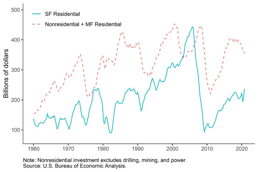
1. Introduction
The construction sector of the economy is inherently cyclical. Figure 1 presents residential and
nonresidential construction investment in the United States from 1960 to 2020 and reveals a
series of large swings for both types of collateral. The bust was especially strong in the Great
Recession, with a peak-to-trough decline of 79 percent for residential investment and 51 percent
for nonresidential and multifamily investment. 4 An important contributor to this high degree of
cyclicality in the construction sector is the stickiness of construction spending, caused by the
time required to plan, finance, and construct a project. Many commercial projects take three or
more years to complete, making it difficult to quickly adjust the level of investment in response
to demand shocks. 5

 Figure 1: Level of Investment in Construction from 1960 to 2020

It is not surprising, then, that construction loans have often played a significant role in
weakening bank balance sheets and contributing to bank failures during periods of financial
distress. 6 Noncurrent loan rates for acquisition, development, and construction (ADC) loans at
U.S. banks were more than double the noncurrent rates of other types of mortgages during both

4
 Residential investment peak is 2005Q4 and trough is 2009Q2, while for nonresidential investment the peak is
2008Q2 and the trough is 2011Q1.
5
 For example, see Grenadier (1995) and Wheaton (2014).
6
 We include in our analysis not only loans for the construction of the actual buildings but also loans to acquire the
land itself and loans to develop the lots before the actual building construction (i.e., putting in curbs and pipes, etc.)
For the remainder of the paper, construction loans refer to the subset of loans that finance the construction of the
actual buildings.

 2

the Great Recession and the 1980 to 1994 banking crisis. 7 Researchers have also found that
banks with heavy exposures to ADC loans were more likely to fail during both crises. 8 More
broadly, periods of real estate speculation have frequently contributed to financial crises around
the world. 9 Thus bankers need to approach ADC loans with appropriate caution and expertise,
and banking regulators need to set policies and procedures that suitably address the risk.

Unfortunately, there is much less information in the literature about what triggers losses for ADC
loans than for retail loans, corporate loans, or mortgages on existing residential and commercial
properties. Other types of loans often use nonbank financing, such as public debt markets or
securitization, that provide publicly available loan performance data for empirical studies. 10
ADC loans instead have, until recently, been limited to bank financing. As a result, data
availability has severely restricted research on ADC loan performance. In fact, we are unaware
of any empirical research that focuses on loss given default (LGD) for ADC loans, despite its
critical importance to the losses of this high-risk asset class.

This paper fills this hole in the literature by using a unique and proprietary set of loan-level data.
The goal of this paper is to learn about the factors that drive distressed LGD for ADC loans and
to explore the implications for lenders and regulators. We decompose LGD on ADC loans into
components that can inform bankers, investors, and regulators about risk exposures in actionable
ways. We then group the explanatory variables into loan, bank, and market characteristics, and
we examine the sensitivity of LGD to each group. Losses due to poor underwriting or poor bank
management can be mitigated through changes in lending policies and supervisory oversight.
Other factors that are not under direct control of the lender, such as losses tied to changes in
market conditions post-origination, are best addressed by loss reserves or capital requirements.

We analyze LGD for a sample of more than 15,000 loans from over 275 failed banks that were
resolved by the FDIC from 2008 to 2013. Most of these loans were originated during the boom
period in the mid-2000s, defaulted during the Great Recession, and were worked out during and
after the Great Recession. We acknowledge that this sample is hardly random: clearly we are
oversampling bad loans at bad banks during a very bad time. 11 However, we feel that this is

7
 Author calculations using Call Report data. From 2008 through 2013, the noncurrent rate for ADC loans peaked at
16.8 percent, single-family peaked at 8.1 percent, and the others (C&I, multifamily, and other CRE) peaked below 5
percent. From 1991 to 1994, ADC loans peaked at 14.1, and the next highest loan type (other CRE) peaked at 5.5
percent. Data are not available for most loan types before 1991.
8
 See GAO (2013) and Friend, Glenos, and Nichols (2013) for analysis of the Great Recession. See Fenn and Cole
(2008) and Collier, Forbush, and Nuxoll (2003) for analysis of the 1980 to 1994 crisis.
9
 Both Kindleberger (2000) and Reinhart and Rogoff (2011) cite speculation in various forms of construction and
real estate as an underlying cause for many historical financial crises.
10
 See, for example, Altman, Resti, and Sironi (2004) and Downs and Xu (2015).
11
 We perform a benchmarking exercise in Appendix B, comparing our data against losses on construction loans
from a separate and independent supervisory data collection for large banks. We find differences between the two
samples, but we also find credible explanations for these difference that relate to the composition of the sample

 3

precisely the sample one would want to work with to explore the drivers of ADC loan risk. It is
losses on bad loans during bad times that account for the majority of ADC losses at banks and
are the most damaging to the banking industry. And it is the drivers of distressed LGDs that is
what is interesting, as aggregate losses on construction loans during benign periods have
historically been negligible.

One of our key findings is that banks exert no direct control over some factors that heavily
influence distressed LGD. More specifically, we find two factors related to local markets at the
time of default: the share of noncurrent ADC loans held by local lenders when the loan defaults,
and the change in the local ratio of ADC loans to total loans between origination and default.
Higher local noncurrent rates for ADC loans at the time of default are an indication of markets
that are experiencing distress. At the same time, an increase in local ADC lending between
origination and default shows the extent to which other lenders are leaning into the market. If a
local area has both strongly increasing ADC lending and relatively high local noncurrent rates at
the same time, the local market may be unstable or overheating. We would expect to observe
higher losses on loans defaulting in these markets. We believe that the sensitivity of losses for
ADC loans to changes in these local market factors post-origination provides a strong argument
supporting the use of higher capital requirements and lower loan-to-value (LTV) limits than for
less cyclically sensitive loans. 12

We document the importance of market conditions at loan origination as well. The bank’s
decisions regarding when and where to make ADC loans are not exogenous: they reflect a bank’s
ability to properly assess and manage risk based on information available when the lending
decision is made. We find that loans originated in markets with higher proportions of ADC loans
to total loans are associated with higher losses, and loans originated in markets with higher ADC
lending growth in the period leading up to origination also have higher losses. Local markets
with outsized ADC lending exposure and faster ADC loan growth at origination may contribute
to higher losses through multiple channels, such as less experienced lending officers and
builders, weaker loan covenants, and less focus on risk exposures. In highly competitive markets,
lenders are well aware that they can originate loans only if their loan terms and covenants are
competitive. They may pay insufficient attention to increases in the supply of homes and
buildings (including the extent of new inventory that will or may soon arrive), optimistic
construction budgets or real estate appraisals, or environmental or other construction risks. Given
the time delay required to complete construction and the inability to adjust investment quickly, a
risk of oversupply under such conditions may be heightened.

(such as size and geography) and variable definitions, increasing our confidence in the representativeness of the
FDIC loan data.
12
 The noncurrent rate for ADC loans, as reported in the Call Report, soared from 0.8 percent as of year-end 2006 to
16.8 percent as of March 31, 2010. The peak rate for ADC loans was more than double the peak rate for other loan
types.

 4

We find that loan characteristics also explain a large share of the variation in LGD. Loans for
projects earlier in the development cycle, specifically those to purchase land and develop lots,
had significantly higher losses than loans for the actual construction of either single-family or
commercial buildings (“vertical” construction). This supports tighter capital and LTV guidance
for these loans. We find that smaller loans in our sample also have higher loss rates. The location
of the project matters, with loans outside of the originating bank’s footprint or in a judicial
foreclosure state 13 having higher losses as well. We do not observe a significant difference in
LGD between single-family and commercial construction loans.

We examine several loan-level characteristics based on the observed performance of the
mortgages post-origination. This includes the timing of the default (specifically the age of the
loan at default) and whether the loan defaulted at the expected maturity of the loan (a “maturity
default”). We also include the share of the committed balance that has been drawn at the time of
default and whether the bank allowed the borrower to draw more than what was originally
committed (an “overage”). These loan-level variables at default reflect a combination of
borrower/builder performance and the monitoring function of the lender. From a collateral
perspective, these variables may reflect the extent of progress made in creating collateral value
through construction.

In contrast to market and loan characteristics, bank-level factors seem to explain much less of the
variation in LGD. These include broad measures that are readily comparable across banks, such
as asset size or portfolio growth, which may, for example, reflect institutional differences in
specialization or in how loans are originated or monitored. We find that larger banks tend to
suffer lower losses in default. We also observe that LGD is higher when the bank had high ADC
loan growth leading up to origination and when it spent a longer time in distress before failure.
But overall, the impact of bank-level characteristics on LGD appears much smaller than loan-
level or market-level characteristics.

Our results have important implications to both bankers and regulators. When the demand (or
speculative demand) for new homes and buildings triggers a sustained strong increase in ADC
lending, the conditions for overbuilding—followed by high ADC defaults and high LGD on
defaulted loans—strengthen. Banks would be well served by astute credit risk functions that are
well informed about the risks that ADC loans pose during periods of distress, and how those
risks are exacerbated when the local market experiences a sustained period of new construction
and high levels of competition. While good underwriting and loan monitoring processes within
the originating bank will mitigate losses during periods of distress, the actions of other local
lenders and builders may contribute to oversupply in the market. Bank examiners should look for
evidence that banks understand these risks, have the appropriate levels of loss reserves, actively

13
 That is, a state where a court order is required for foreclosures.

 5

monitor for potential overbuilding, and do—or stand ready to—pull back their lending or
promptly take other actions to reduce their exposures as risks increase.

The rest of the paper is organized as follows. Because lending related to construction has unique
traits that influence LGD, Section 2 provides institutional background information that informs
our analysis. Section 3 discusses the FDIC Loss Share Administration program and the data used
for our analysis. Section 4 lays out the methodology, Section 5 provides the results, and Section
6 discusses the implications of those results. Section 7 concludes.

2. Institutional Background
Several unique aspects of ADC loans set them apart from other mortgages. The most significant
difference from the perspective of modeling losses is that a large share of the collateral that
backs ADC loans is created during the loan term. There is no cash flow from rents available to
service the debt. There is no rental history upon which to base a valuation, merely a speculative
estimate of value based on market conditions as of the expected completion date. This is a
foundational difference that influences the loan origination and servicing processes, the loan
terms, and the lender’s risk exposure. Section 2.1 begins by explaining the processes involved in
originating and managing these loans and the loan terms. Section 2.2 discusses the lender’s risks
from ADC loans and how they relate to the nature of the collateral, the loan administration
processes, and the loan terms. In both sections, ADC loans are compared with other, more
familiar, types of real estate loans, 14 and relevant academic literature is discussed.

2.1 Loan Processes and Terms
This section begins with a discussion of the typical loan origination process and loan terms,
followed by sections on the collateral valuation at origination, the monitoring process, default,
and the loan workout process. 15

2.1.1 Loan Origination and Loan Terms
Investors frequently form a Limited Liability Corporation (LLC) for each specific project. The
LLC acts as the official borrower, who hires a builder to do the construction; sometimes the
builder is the investor. The investor normally purchases the property and places it in the LLC (if
any), designs the construction project, hires the builders, and completes the entitlement process 16
before origination.

The term to maturity for ADC loans is relatively short, and larger projects usually involve
multiple loans. For example, for a single-family housing development, the borrower might obtain
a land development loan to put in curbs, underground pipes, and electrical service and a separate

14
 Specifically, to a typical first lien for a single-family home or commercial real estate loan (CRE) loan.
15
 This section is based on anecdotal information from discussions with bankers, examiners, and other experts.
16
 That is, the process of obtaining the zoning changes and other regulatory approvals that are required before
construction begins.

 6

construction loan to build the houses. Even single construction loans are often structured in
tranches, with the next segment of the committed balance being issued to the borrower only if
certain thresholds are met. For larger office/retail complexes, there may be separate loans or loan
tranches for each phase of development. Many ADC loans include a “permanent” (that is, long-
term) financing phase once construction is complete and other thresholds are met. 17 A large
share of the profits come from fees at origination. The loan structures for other types of
mortgages are more permanent and less complex, with interest income comprising a larger share
of the lender’s profit.

ADC projects rarely produce income for the borrower until construction is complete and the
property is either leased to tenants or sold. Therefore, the loans are normally structured with an
interest reserve with no payments due directly from the borrower until maturity (or, in the case of
single-family developments, as homes are sold). With an interest reserve, the total amount of the
loan includes funds disbursed to the borrower and undisbursed funds that are used to cover
interest expenses during the loan term. This structure contrasts with other types of mortgages,
where regular payments are due throughout the loan term (and which serve as a key measure in
determining default).

The payment stream to the borrower also differs markedly from other mortgages. For single-
family residential (SFR) and commercial real estate (CRE) mortgages, the full loan amount is
normally disbursed at origination. For ADC loans, the loan documents set forth a pre-defined
schedule, where new disbursements are made as various phases of construction (or in some cases
sales or leases) are completed. The requirements for each tranche of the loan to be disbursed are
spelled out in the loan covenants. Disbursements are often relatively modest during the early part
of the loan term.

One other significant difference between ADC loans and other mortgages is the prevalence of
recourse. Lenders frequently require borrowers to provide personal guarantees to back ADC
loans. These guarantees, or recourse, provide some “skin-in-the-game” on the part of the
borrower, if the value of the raw land or partially built project that is pledged as collateral is not
sufficient. Recourse is less frequently used for other types of mortgages, where the equity share
of the existing property pledged as collateral provides the “skin-in-the-game.” Glancy, et al.
(2021) find that recourse in transitional loans (defined as construction and redevelopment loans)
is correlated with unobserved risks, as transitional loans with recourse have higher spreads at
origination and worse performance during the COVID pandemic, however they are looking at
the impact of recourse on default and not recovery rates.

17
 For example, for a multifamily loan, a specified share of the apartments might have to be leased.

 7

2.1.2 Valuation at Origination
Banks must decide whether to originate an ADC loan based on the potential value of the project,
which is by definition unobserved. Third-party certified appraisers are hired during the loan
approval process and must adhere to well-developed standards that govern estimation methods
and the products they produce. 18 Loan commitments often occur before the appraisal is
complete—and are often conditional on the appraised value—but loan originations always occur
after the appraisal. Appraisals for construction projects are by their nature more speculative than
for existing buildings, where historical rental cash flows are available.

Banks normally request both an “as is” appraised value and one or more “as will be” appraised
value(s). There are two standard “as will be” measures of value. The first, known as “as
stabilized” value, represents the value for the finished project when the appraiser assumes that
the property is already built and leases have stabilized or finished lots or homes have been sold
as of the appraisal date. The second, known as the bulk value, represents a value based on a
discounted cash flow approach when the appraiser develops assumptions about the time needed
for building, the time needed for lease stabilization or asset sale(s), the future value of the
finished project, and then discounted the estimated future value to the appraisal date. Finished
product values are invariably higher, and banks used them more often—and relied on them more
heavily—during boom periods. We expect that, especially when markets are shifting, the
appraisals are significantly less reliable for construction projects than for other real estate.

2.1.3 Loan Monitoring
The monitoring process for ADC loans is much more labor intensive than for other mortgages
and often requires detailed knowledge of construction, the local regulatory approval process, the
loan contract details, the local market, and the title insurance process. Over the term of the loan,
the lender monitors the progress of the construction, including items such as the receipt of
materials, payments to suppliers, progress on the building(s), and associated regulatory
approvals. Based on the status of the construction and the loan covenants, the lender determines
when draws can be made, the size of the allowed draws, whether and how the loan terms should
be adjusted (if construction problems arise or markets shift), and when payments are due.
Adjustments are commonplace as the construction progresses and may arise because of issues
such as changing prices for labor or materials, delays in receiving materials, subcontractor
availability, environmental problems, poor quality construction, or changes in local demand.

2.1.4 Loan Default
The timing of loan default falls into two categories: term defaults and maturity defaults. Maturity
defaults occur when the borrower is unable to sell the collateral at an adequate price, or, for
commercial properties, when the borrower cannot obtain sufficient permanent financing to pay

18
 See Appraisal Standards Board (2017) for details.

 8

off the ADC loan in full. 19 Because the borrower does not make regular payments, term
defaults 20 are almost always determined by the lender (or in some cases bank examiners); they
are frequently based on an evaluation of the local market conditions and anticipated demand, or
on the borrower being unable to meet performance covenants. This contrasts sharply with other
types of mortgages, where borrowers make regular payments and default is simply determined
by payment delinquency. 21 Because loan default involves judgment on the part of the bank, the
timing may be less consistent across banks for ADC loans. 22

2.1.5 Loan Workout
The workout process for ADC loans is more complex and the lender’s negotiating position is
weaker than in the other types of mortgages, for two reasons. First, the investor’s equity position
is more likely to be deeply negative, especially during a severe crisis. 23 Thus investors may be
unwilling or unable to bring additional capital to the project or monitor the building process.
Second, and more importantly, the builder has considerable scope to influence the outcome and
incentives that rarely align with those of the lender. The construction industry is highly cyclical,
and during distress periods builders are retrenching and desperate for cash to pay staff and fund
operations. With no new construction projects available, builders aggressively seek additional
draws from existing loans to survive. They rarely have any reason to cut back on existing
projects, regardless of whether demand exists for the finished project. All the loan participants
are well aware of the high cost of changing builders in the middle of a project and the significant
discount to market value for an incomplete building, and builders and investors can use that
knowledge at the lender’s expense during negotiations.

2.2 Risks
We now link some of the institutional aspects of ADC lending to specific risks that can help
drive losses. We divide these risks into four separate, but often interrelated, topics: construction
risks, the opacity of ADC loans, the option value of land, and sensitivity to real estate cycles.
Both construction risks and opacity contribute to the higher level of idiosyncratic risk of
construction loans, while the option value of land and the sensitivity to real estate cycles
contribute to the higher level of cyclical risks for ADC loans. We provide a summary of risks in
Appendix A.

19
 In some cases, this takes the form of being unable to meet the lender’s requirements for a conversion to permanent
financing (that is a conversion to a CRE loan).
20
 Term defaults occur before the maturity of the loan. We define maturity defaults as defaults that occur within 90
days of maturity or after maturity. All other defaults are term defaults.
21
 In some cases, lenders may place CRE loans into nonaccrual status even when payments are current, because the
value of the collateral has dropped and the lender no longer expects full repayment of the loan at maturity. This is
common in the commercial mortgage-backed securities (CMBS) market, where the master servicer will transfer
such a loan to the special servicer to begin the loan workout process even if the loan is still current.
22
 However, banks have some scope to restructure other types of troubled loans in ways that minimize reported
defaults, known as “evergreening.” This type of restructuring is less likely to occur for single-family mortgages
because most of them have standard terms.
23
 In some cases, solvency may be uncertain or positive but the investor is illiquid.

 9

2.2.1 Construction Risks
Cost overruns for construction projects are commonplace. Problems often begin with the budget
itself, which may suffer from optimism bias, inadequate feasibility analysis, omissions of
required items, or simplistic assumptions that do not adequately consider risks or entrepreneurial
profit. Other problems can include bad weather; delays in the availability of subcontractors, staff,
materials, or government inspectors; design changes and scope creep; cost increases for labor or
materials; unexpected underground conditions and other environmental problems; inexperienced
builders; or foul play and corruption. 24 The potential for these challenges to arise results in the
need for ongoing, and costly, monitoring of ADC loans by the lender.

2.2.2 Opacity
As discussed in Section 2.1, the lending function for ADC loans involves more complicated
terms and conditions than for other types of mortgages. The loan monitoring process is more
complex, and determining whether the loan is in default is more ambiguous. The loan workout
process is more likely to depend on stakeholders with incentives that differ markedly from the
lender. Loan guarantees are used more frequently, and the value of these guarantees are not
readily discernable. The appraisal process requires more estimation that introduces more
opportunities for error, and the construction process involves numerous potential pitfalls that are
not immediately obvious. Taken as a whole, these characteristics support a conclusion that ADC
loans are more opaque than other mortgage types. This opacity explains why there is no
standardized underwriting process and why banks usually retain ADC loans in their portfolios. It
also may magnify the scope for lender myopia or overconfidence.

2.2.3 Option Value of Land
A wide range of research exists on the option value of land, from Quigg (1993) to Munneke and
Womack (2020). The underlying theory is that all land, both developed and undeveloped, is
valued based on its highest and best use. Geltner et al. (2014) documented how the highest and
best use may change over time in response to changes in the local market and demand for space.
Property whose highest and best use was as a farm may instead now have a highest and best use
as single-family residences. Once the option value of developing the land (or redeveloping it to
change the property type) reaches a certain threshold, the project becomes viable and can acquire
investment and financing.

One aspect of the option value of land that is relevant to thinking about potential loss on
construction loans is the limited reversibility of investment. When the project starts, the highest
and best use might be single-family residential. However, once the project reaches completion,
the highest and best use may have shifted due to market developments and is now retail. The

24
 See Ahiaga-Dagbui and Smith (2014) for additional discussion.

 10

physical aspects of the project are difficult to reverse: for example, the street plan for a housing
development would not serve an office park.

But zoning restrictions can often be even more difficult to reverse. Before loan origination,
builders must obtain local approvals to construct the building(s) and, for single-family
developments, break the property into separate lots for future sale, which is often time-
consuming and politically challenging. This process can add substantial value to the project: on a
per-acre basis, the value of timberland or farmland is often a fraction of the value of the same
acreage (in the same condition and location) that has been approved for homes or a retail
shopping center. But it also represents a stickiness in terms of optimal land use. For example, if
agricultural land had been re-zoned as residential, it could be costly—or politically impossible—
to transition it to another higher best use. The option value of the land is “spent” once the project
has begun. A shift in demand during a project’s lifetime could lead to higher losses on the ADC
loan.

2.2.4 Sensitivity to Real Estate Cycles
LGD for ADC loans is far more sensitive to real estate price changes than other types of
mortgages, for several reasons. First, substantial time elapses between the date the lender
commits to the loan and completion of the construction. This lag is caused by the time to build,
which is often longer than the original estimate because of time lost to address supply problems
and subcontractor schedules, longer-than expected regulatory approvals (such as demolition,
environmental impact, various stages of construction, and sometimes zoning), and investor and
lender decisions associated with change requests, and lender inspections and approvals for
draws. Major market shifts can occur between the loan commitment date and the completion of
construction. 25 The potential for losses relating to the time delay between origination and
completion is compounded by two additional factors: (a) strong incentives for builders to
continue building during periods of distress regardless of the declining value of the finished
product, and (b) potential weaknesses in appraisals, such as reliance on “as stabilized”
valuations.

Second, most construction projects end with empty buildings, and the borrower’s ability to repay
the loan is generally contingent on finding buyers or tenants for the finished product. 26
Relocation costs, and the transaction costs for purchasing real estate, are substantial and may
hinder sales or leases. Relatively few ADC loans are backed by owner-occupied buildings or
projects with significant levels of pre-leasing or pre-sale contracts in place at the time of loan
commitment. During periods of serious distress, pre-leasing and pre-sale agreements can fall

25
 See Grenadier (1995) and Wheaton (1999) for additional discussion. Both authors cite this time lapse as a
contributing factor to real estate cycles.
26
 Or, for horizontal construction, approval of a new loan for the next phase of construction.

 11

through. On the other hand, many commercial leases are long-term. These phenomena mitigate
losses for other types of residential and commercial mortgages but amplify the sensitivity to
business cycles for ADC loans. 27

Third, while all loan types are affected by heightened competition during boom periods, ADC
loans tend to be more strongly affected. ADC loan growth was much stronger than other loan
types during the boom before the Great Recession: from year-end 2003 to year-end 2007, ADC
loans held by banks increased 131 percent, but other types of mortgages held by banks increased
45 percent. 28 Lenders with a stronger appetite for growth—and thus a higher willingness to take
on risk—gravitated to ADC loans, most likely because it was easier for them to gain market
share. 29 For example, as of year-end 2007, the median ratio of ADC loans to total loans held by
de novo banks was 17 percent; the ratio was only 5 percent for banks that were ten years old or
older and had the strongest CAMELS composite rating. 30 During boom periods, lenders may feel
pressure to grow quickly, and the benefits of monitoring (including tight loan covenants)
diminish while the costs remain constant. 31 In addition, the average experience levels of lending
officers and builders declines. New builders are more likely to make mistakes, both in the cost
estimation process and the construction itself. New lending officers have less knowledge of and
skill in all aspects of the loan origination process, and they lack memories of the high costs
associated with real estate downturns. Lusht and Leidenberger (1979) found empirical evidence
that both builder and lending officer experience reduced the probability of default for
construction loans; there is good reason to expect the same for LGD. 32

3. Data
This section introduces the FDIC Loss Share Administration data that are the primary data used
in the paper. We then discuss the construction of our LGD measure, including a decomposition
of the loss into different components. The decomposition supports the comparison of our LGDs
with those from other sources that may contain different components. We then provide a range of

27
 See Grenadier (1995) for additional discussion.
28
 Percentages derived from bank Call Reports. See Rajan (1994) for additional discussion and evidence that
heightened competition results in looser bank lending policies (such as relaxed underwriting criteria and less
stringent monitoring).
29
 According to bank Call Reports, as of year-end 2006 (at the height of the boom), de novo banks, banks with high
loan growth rates, and banks that relied heavily on brokered deposits all had higher concentrations of ADC loans
and higher ADC loan growth rates than other banks. Yom (2005) discusses the incentives for de novo banks to grow
quickly.
30
 Data from bank Call Reports and examinations. De novo is defined as eight years old or younger. For the second
group, only banks with a CAMELS composite rating of 1 are included in the calculation. CAMELS ratings are
supervisory designations of bank condition and range from 1 (very strong) to 5 (very weak).
31
 At least as long as the boom continues. See Rajan (1994) and Levitin and Wachter (2013) for evidence and
discussion on pressure for earnings and asset growth during boom times. See Ruckes (2004) for an analysis of the
net benefit of loan monitoring across the cycle.
32
 There is substantial evidence of the same phenomenon for lending more generally. See, for example, Berger and
Udell (2003) and Rötheli (2012).

 12

descriptive statistics about our loss data, both overall and across different regions and property
types. 33 We end with a brief discussion of potential concerns about our data.

3.1 FDIC Loss Share Administration Data
In this study, we use LGD data from banks that failed and were resolved by the FDIC in the
aftermath of the 2008 financial crisis. Loan portfolios held by failed banks oversample the upper
end of the credit loss distribution of ADC loans, and they should incur higher default rates than
portfolios at healthy banks. The nature of this sample selection works to our benefit. A signi-
ficant driver of losses to a bank will depend on the performance of the worst-performing loans in
their portfolio. A lending institution’s solvency is not dependent on the performance of the
median loan, but by the performance and losses in the upper tail of the credit loss distribution.34

The FDIC has a loss share program to help dispose of assets from failed banks. From 2008
through 2013, the FDIC sold $39 billion in ADC loans from 289 failed banks to 144 bank
acquirers with loss share coverage. Most of the FDIC loss share agreements provided the
acquirers with 80 percent indemnification from credit losses for five years for assets covered
under the agreement (thus acquirers would absorb just 20 percent of the losses). 35 To manage its
risk exposure and support program administration, the FDIC collected information from the
failed banks as of the sale date (that is, the date the bank failed) and through detailed quarterly
reporting requirements from the acquiring banks after the sale date. Note that when we refer to
bank characteristics in this paper, we are referring to the characteristics of the failed bank that
originated the loan and not the acquiring bank that serviced the loan. The dataset contains data
from the inception of the program in 2008 through year-end 2015. 36

One of the unique aspects of the loss share program data is its detail on the components of the
losses. As we discuss further in Section 3.2, most existing LGD data in the literature do not have
this level of detail. Loss share LGD components include
 • Charge-offs (net of recoveries);
 • Loss on sale of asset (loan or other real estate owned (ORE));
 • Expenses (legal fees, foreclosure expenses, appraisals, property maintenance costs, etc.)
 paid to third parties related to the asset, except servicing fees; and
 • Up to 90 days of accrued interest.

33
 Given that the loan level data we use are by definition drawn from failed banks, Appendix B provides a
benchmarking exercise with a separate and independent set of data on defaulted construction loans from the Federal
Reserve’s FR Y-14Q Schedule H.2.
34
 Compared with surviving banks, failed banks had higher ratios of ADC loan exposure to capital and higher loan
default rates during the Great Recession. This does not necessarily mean that they had higher LGDs. We tested
whether the individual bank’s loan default rate influenced LGD for our sample, and we found that the relationship
between LGD and the bank’s default rate was insignificant in most specifications.
35
 For an additional three years, the acquirer was required to continue reporting all losses and recoveries, and to
continue to share recoveries (net of certain collection expenses) with the FDIC. However, most of the loss share
transactions were terminated shortly before or after the full indemnification period ended.
36
 As of year-end 2015, either the loss share agreements had been terminated or the loss-sharing period had expired
for 243 of the 289 agreements. Only $860 million (2 percent) of the ADC loan portfolio was still active.

 13

For loans foreclosed under the loss share program, the FDIC was entitled to share in any income
earned from the collateral. Losses from bulk loan sales were covered by the FDIC, but only if the
acquirer could demonstrate that a bulk loan sale was more cost-effective than loan-level (or
borrower-level) workout strategies. Therefore, bulk loan sales were rare.

The loans in our sample were originated by banks that failed. When the originating bank failed,
the loan underwent an ownership change during the loan term or workout period. This is not a
random sample of all defaulted ADC loans in the United States during the relevant time horizon.
To address concerns that our sample may not be representative of defaulted ADC loans at
privately held banks, we note that almost all of these loans were originated when the originating
banks were healthy and when there was substantial industry-wide growth in ADC loans. In
addition, Shibut and Singer (2015) compared LGD using similar data for commercial real estate
(CRE) loans backed by completed buildings from the FDIC’s loss share program to LGDs
reported in studies that relied on public sources (i.e., not failed banks). After presenting results
from multiple studies, they concluded that “the LGDs in this sample are generally consistent
with other studies that focus on periods of distress.” 37 We also compare our sample to a group of
distressed ADC loans at large banks and conclude that the FDIC data seem consistent with the
Y-14 data in several ways (see Appendix B).

We considered the possibility that the FDIC indemnification under the loss share program might
weaken the incentives of acquirers to work out assets effectively when compared with assets that
lack indemnification coverage. The FDIC took several actions to mitigate the potential effects.
First, it required that acquirers work out covered assets in the same way that they work out their
own assets. Second, it required regular standardized reporting, adequate workpapers, and
evidence that the loans were worked out effectively. Third, it reviewed loss claims and
performed on-site compliance reviews at least once a year. The FDIC had the right to demand
program improvements, reverse loss claims or, in the case of a serious contract breach, abrogate
the loss share coverage altogether. 38 These factors help mitigate any bias due to the incentive
created by the loss sharing agreement.

We drop loans from the sample for several reasons. Loans are dropped if the asset had not yet
been extinguished (that is, the asset is sold, paid off, or written off in full) when the loss share

37
 Shibut and Singer (2015), p. 11, with additional discussion on p. 10. The authors note that close comparisons are
not available, but they include LGDs calculated from defaulted commercial mortgage-backed securities and CRE
loans held by life insurance companies.
38
 These are just some of the FDIC’s options to manage its exposure. Acquirers have the right to contest any FDIC
action. For more details about the loss share program, see www.fdic.gov. All agreements are posted in the failed
bank section. See also FDIC (2010) for details about the data collected from acquirers and FDIC Office of Inspector
General (2013) for additional discussion about the FDIC’s monitoring program and its effectiveness.

 14

agreement was terminated or at the end of sample period (right-censoring), 39 or because of data
problems associated with loans that defaulted before the bank failed. Loans that defaulted well
before failure are omitted from the sample. 40 Loans are also dropped if they are from a U.S.
territory (primarily Puerto Rico) or a foreign country, if they had very small outstanding loan
balances at default ($100 or less), or because of other missing data. 41

3.2 Key Definitions
Our definition of LGD is based on a combination of the guidance on LGD for the Basel 2
Advanced Approach models and data availability. The definition is as follows:

 = ( − + )/ 

EAD is the exposure at default, defined as the total drawn and undrawn balance committed on
the loan at the time of default; REC is the discounted net principal recovery on the loan; EXP are
the discounted expenses consisting of legal fees, foreclosure expenses, appraisal fees, property
preservation costs, property taxes, and so on, plus up to 90 days of accrued interest at the time of
default. Acquirers do not report all the cash inflows under the loss share program, but they report
principal losses and expenses. Therefore, we back out the discounted principal recovery REC as
the exposure at default EAD minus charge-offs CO (net of recoveries) and any loss on sale of the
asset LOSALE, all discounted as of the default date at the interest rate on the loan: =
 − − . 42 Like many studies, our definition excludes two items that are included
in the definition in the Basel 2 framework: servicing costs 43 and unpaid fee income. To guard

39
 The notion of “resolution bias” suggests defaulted loans that are extinguished quickly tend to have lower losses,
so an exclusion of longer workouts outside our sample period would tend to bias LGD downward. However, failed
bank acquirers had strong incentives to complete the workout for defaulted loans before the loss share coverage
terminated, particularly for defaults with larger anticipated losses. We therefore do not believe that resolution bias is
likely to be an issue in our sample.
40
 Some banks retain data on charge-offs in their loan servicing system for only a year after charge-offs are taken.
Thus, loans that defaulted more than a year before failure are omitted because we are uncertain that the historical
charge-off information is complete.
41
 Specifically, observations were also dropped if (a) the asset type was uncertain, (b) there were math errors in the
acquirer’s loss submissions or the FDIC’s corrections of those submissions, (c) the ADC loan was combined with
other types of loans during the workout process, or; (d) data for explanatory variables (or data needed to calculate
explanatory variables, such as location of the collateral) were missing or incoherent. Also, note that some items were
estimated, notably the type of collateral and stage of development (which were estimated using heuristic methods
applied to relevant text data fields).
42
 The Basel 2 framework requires discounting to the default date using a market rate. There is no strong consensus
on the appropriate interest rate, but the loan rate is frequently used. See Maclachlan (2004) for additional discussion
and a survey of discounting methods used in academic research on loan losses.
43
 The Financial Crisis Inquiry Commission noted that a special servicer that handles problem loans “typically earns
a management fee of 25 to 50 basis points on the outstanding principal balance of a loan in default as well as 75
basis points to one percent of the new recovery of funds.” See Financial Crisis Inquiry Commission (2010), p 44.
The Commission discussed servicing arrangements for loans that collateralize CMBSs. Servicing costs for
construction loans might be different.

 15

against potential reporting errors, we winsorize observed LGD in our sample at the 99th
percentile.

A key aspect of any LGD definition is how defaults are measured. In our study, we define
default as occurring the first time that we observe any of the following:
 • The loan became 90 days or more delinquent,
 • The loan was placed in non-accrual status,
 • The loan was classified as being in foreclosure or bankruptcy, or
 • A charge-off was taken on the loan, or any claim was made under the loss share program.

Figure 2 shows our sample distribution of LGD. Only 16 percent of the defaulted loans avoid
losses altogether, and 15 percent have losses of 100 percent or more. Had we constrained LGD to
be no higher than 100 percent, Figure 2 would look similar to the “U” shape seen in many
studies of realized losses. 44 We observe in our sample many loans with losses exceeding 100
percent. LDGs above 100 percent typically occur when expenses are significant and principal
recoveries are small. Such loans tend to be small (median EAD of $87,000, versus $260,000 for
the others), are more likely to be foreclosed (56 percent, versus 44 percent for the others), and
have longer workout periods (median of 11 quarters, versus 7 quarters for the others).

 Figure 2: Sample Distribution of LGD
 4000
 3000
 Frequency
 2000
 1000
 0

 0 .5 1 1.5
 LGD

One contribution of our paper is that it uses a detailed measure of LGD that captures nearly the
full range of costs a lender would incur in resolving a defaulted ADC loan. Many studies of
losses on CRE mortgages are limited in their data on the composition of losses, and are limited to
comparing market price reactions to default announcements for CMBS securities or the
subsequent sales price of the property to loan exposure at default. We show in Figure 3 the
decomposition of LGD across different buckets of LGD losses. This breakdown shows how
expenses, the top (dark blue) segment in each column, account for a significant share of total
losses across the loss distribution. For loans with very small positive LGDs, expenses comprise

44
 See Araten et al. (2004) and Asarnow and Edwards (1995) for examples of realized loss distributions.

 16

more than 20 percent of losses. Charge-offs (COs) occasionally reflect the impact of successful
downstream recoveries. In some cases, they even offset some of the losses from expenses and
discounting, which is noticeable in the negative values for owned real estate charge-offs (ORE
COs) in the first three bars of Figure 3. For the segment with losses greater than 100 percent, the
share of expenses is approximately 17 percent of the total losses, highlighting the importance of
using loss measures that include expenses. The share of losses associated with charge-offs after
the bank has assumed ownership of the property—the ORE COs—increases as losses approach
and exceed 100 percent. ORE COs represents another 15 percent of the total losses for high LGD
loans in our sample, indicating that a significant portion of the total loss is being recognized later
in the workout process. LGD estimates that do not consider expenses related to assets in default,
or subsequent charge-offs for ORE assets, later in the workout are likely to underestimate the
extent of true losses incurred.

 Figure 3: Decomposition of Net Losses by LGD Category
 100%

 80%

 60%

 Expenses
 40%
 Discounting
 Loss on Sale
 20%
 Net ORE COs

 0% Net Loan COs
 10 20 30 40 50 60 70 80 90 100 130
 -20%
 LGD Category *
 * 10 includes 1% < LGD =< 10%, 20 includes 10% < LGD =< 20%, etc. CO stands for charge-offs, net
 of recoveries.
 Source: FDIC loss share and failed bank data.

3.3 Descriptive Statistics
This section begins with basic descriptive statistics across the full sample. We then provide
additional detail on key variables and a breakdown of the sample based on geography and type of
collateral.

3.3.1 Full sample characteristics
As shown in Figure 4a, most of our loan originations occurred between 2005 and 2010, with 25
percent occurring in 2007 and 63 percent occurring between 2006 and 2008. 45 One interesting
aspect of the origination dates is that it includes a non-trivial share of construction loans
originated during the financial crisis, when overall construction lending dropped significantly.
Most defaults occurred between 2009 and 2011, with 33 percent in 2009, 29 percent in 2010, and
15 percent in 2011. This is clearly a sample of loans that defaulted during a period of severe

45
 Observations where either the origination date or the default date are missing are excluded.

 17

distress, which is exactly when losses on construction loans are of greatest concern for lenders
and the broader economy.

Figure 4b shows the distribution of the term to maturity at origination. The mean term to
maturity is 4 years, and the mean age at default is 3.2 years. 46 In addition, 60 percent of the loans
are maturity defaults. 47 Assuming the project has progressed as expected, a default occurring at
maturity would suggest that a bank would have a complete or nearly complete project to seize as
collateral, instead of a partially complete project with greatly reduced value.

Figure 4a: Distribution of Origination and Default Date Figure 4b: Distribution of Term to Maturity

Figure 5 reports the distribution by asset size. The distribution is strongly skewed, with a large
number of smaller assets that relate to construction of individual single-family properties, and is
not dominated by large construction loans for single-family developments or large commercial
projects. This is due in part to the nature of the crisis itself, which was strongly associated with a
boom-bust cycle in single-family lending. It is also due in part to the nature of failed banks,
many of which were smaller institutions specializing in smaller single-family and commercial
construction projects rather than larger residential or commercial developments. It is possible, for
example, that the experience of builders or the structure of financing for those large-scale
projects could differ in certain ways from most of the defaulted loans in our sample. Our results
from this crisis should be interpreted with this in mind.

46
 The average length of the loan is significantly longer than the time it takes to complete a single residential unit,
which is 7.8 months. The difference between the loan term and typical construction period reflects the additional
time built into the loan for preparation before vertical construction, the construction of multiple buildings financed
by the same loan, the construction of buildings with more than a single unit (where the average time to build is 17.4
months), and time required to sell the completed properties.
47
 A maturity default is defined as a default that occurs within 90 days of the scheduled maturity or after maturity.

 18

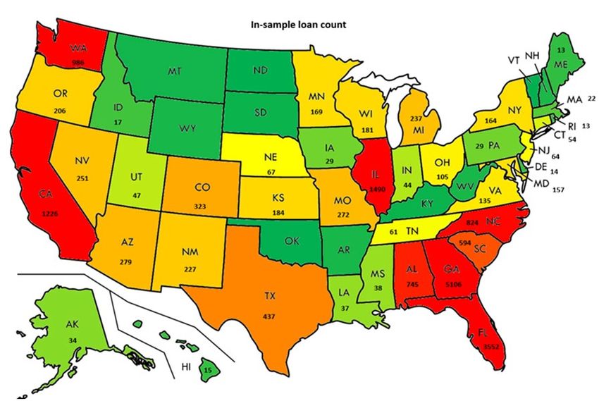
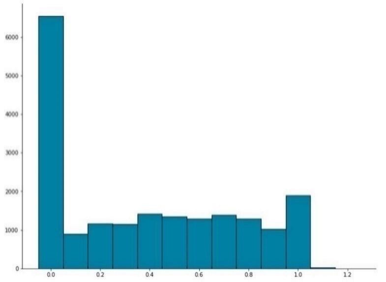
Figure 5: Sample Distribution of Asset Size

Table 1 reports descriptive statistics for the full sample. The first section of the table provides
data on the characteristics of the loans. The mean LGD is 56.7 percent, and the median is 62.4
percent. Defaulted loans with a positive loss for the lender make up 84.4 percent of the sample,
while 15.6 percent of the defaults resolve with no loss. As shown in Figure 5, the distribution of
the size of the loans is heavily skewed: although the mean exposure at default is $1.06 million,
the median is only $230,000. The median interest rate is 6 percent. And as mentioned previously,
the mean term to maturity at origination is four years, and the median is three years. The mean
age of the loan at default is about three years, and 60 percent are maturity defaults. About 37
percent of the sample was already in default when the originating bank failed, and 46 percent of
the loans were foreclosed during the workout period. The mean workout period is 25 months,
and it varies substantially across the sample. The legal process for foreclosure influences the
ability of lenders to seize assets and may be relevant to explain loan loss, so we look at whether
loans are in judicial foreclosure states (41 percent). 48 Construction lending is also an
informationally intensive business, where knowledge of local market conditions are important,
so we track whether loans are made outside of Core-Based Statistical Areas (CBSAs) in which
the originating bank has a branch presence (“out-of-territory”). About 25 percent of the loans
were made based on collateral located outside of the lender’s CBSA footprint; these are not
distributed evenly across regions or banks. For 9 percent of the loans, the outstanding loan
balance exceeded the initial loan amount at some point during the loss share period (thus
indicating that the acquiring bank authorized additional funds to minimize losses).

48
 In judicial foreclosure states, foreclosure requires a court order.

 19

Table 1: Descriptive Statistics for the Sample
 No. of 10th 90th Standard
 Variable Obs Percentile Median Percentile Mean Deviation
 Basel LGD based on discounted loss share cash flows 19,427 0 0.624 1.015 0.567 0.383
 1 if basel LGD has a nonzero loss 19,427 0 1 1 0.844 0.363
 Loan Characteristics
 Outstanding balance at default ($1,000) 19,427 31 230 2,658 1,056 2,598
 Interest Rate 19,427 4.0 6.0 8.5 6.3 2.3
 Term to maturity (years) 18,658 1.0 3.0 7.0 4.0 3.84
 Age at default (years) 18,780 0.93 2.82 5.69 3.17 2.12
 Maturity default* 18,661 0 1 1 0.60 0.49
 In default when the bank failed 18,639 0 0 1 0.37 0.48
 Foreclosed 19,427 0 0 1 0.46 0.50
 Workout period (months) 19,427 3.5 23.5 50.4 25.3 17.9
 Ratio of balance drawn to total exposure ** 19,427 1 1 1 0.95 0.14
 Land development loan 9,286 0 1 1 0.89 0.32
 Judicial foreclosure state 18,493 0 0 1 0.42 0.49
 Out of territory loan (CBSA) 17,775 0 0 1 0.25 0.43
 Overage (Asset bal > init exposure at any time) 19,427 0 0 0 0.09 0.29
 Bank Characteristics
 Bank 3-yr ADC loan growth rate at loan origination 19,427 0 1.25 4.00 1.67 1.42
 CAMELS rating at origination 18,549 2 2 4 2.49 1.05
 Asset size of failed bank at loan origination ($ millions) + 18,714 3,389 6,574
 Failed bank time spent in distress (years) 19,427 0.45 1.18 2.10 1.27 0.66
 Market Characteristics
 Local ratio of ADC to total lending at origination 18,487 0.063 0.117 0.190 0.123 0.051
 Local NC rate for ADC loans at origination 18,481 0.002 0.013 0.153 0.048 0.064
 Local 3-yr change in ADC to total lending at origination 18,481 -0.026 0.025 0.075 0.024 0.042
 Local 3-yr change in brokered to total deposits at orig 18,481 -0.020 0.022 0.058 0.020 0.041
 One year pct point chg in SFR permits/total stock at orig 18,472 -0.004 -0.002 0.001 -0.002 0.002
 Local average vacancy rate for CRE at orig 18,449 0.056 0.081 0.106 0.081 0.020
 Local change in ADC to total lending (orig to def) 16,287 -0.090 -0.032 0.004 -0.037 0.038
 Local NC rate for ADC loans at default 18,501 0.084 0.168 0.223 0.162 0.057
 Change in local ratio of NC ADC to total loans 18,481 0.012 0.119 0.205 0.114 0.076
 * Default was within 90 days of scheduled maturity or after maturity
 ** Capped at 100%
 + Percentile items omitted for privacy reasons
 NC stands for noncurrent (including nonaccrual). SFR stands for single family residential.

The next section of the table looks at the characteristics of the banks in our sample. Growth in
the originating banks’ ADC portfolios was strong during the period leading up to origination: on
average, it was 36 percent in the previous year and 167 percent in the previous three years. The
mean CAMELS rating at origination is 2.49, and the median is 2. The mean size of the failed
banks at origination is $3.4 billion, and the median is somewhat less than $1 billion. We also
track the time the originating bank spends in distress (defined as having a CAMELS composite
rating of 4 or 5). If a bank is closed shortly after it begins to experience distress, then the loans
are more quickly transferred to a healthier institution, which may result in lower losses. In our
sample, the average time spent by the originating bank in distress is just over 1.5 years.

 20