Deep Learning Jet Image as a Probe of Light Higgsino Dark Matter at the LHC
←
→
Page content transcription
If your browser does not render page correctly, please read the page content below
Deep Learning Jet Image as a Probe of Light Higgsino Dark
                                                                                   Matter at the LHC

                                                                     Huifang Lv,1, ∗ Daohan Wang,2, 3, † and Lei Wu1, ‡
                                                             1
                                                                 Department of Physics and Institute of Theoretical Physics,
                                                                          Nanjing Normal University, Nanjing, China
                                                  2
                                                      CAS Key Laboratory of Theoretical Physics, Institute of Theoretical Physics,
arXiv:2203.14569v2 [hep-ph] 15 Apr 2022

                                                                   Chinese Academy of Sciences, Beijing 100190, China
                                                                    3
                                                                        School of Physical Sciences, University of Chinese
                                                                          Academy of Sciences, Beijing 100049, China

                                                                                           Abstract
                                              Higgsino in supersymmetric standard models can play the role of dark matter particle. In
                                          conjunction with the naturalness criterion, the higgsino mass parameter is expected to be around
                                          the electroweak scale. In this work, we explore the potential of probing the nearly degenerate light
                                          higgsinos with machine learning at the LHC. By representing the jets as 2D images, we use the
                                          convolutional neural network (CNN) to enhance the signal significance. We find that our deep
                                          learning jet image method can improve the previous result based on the conventional cut-flow by
                                          about a factor of two at the High-Luminosity LHC.

                                          ∗
                                              lvhf@njnu.edu.cn
                                          †
                                              wangdaohan@itp.ac.cn
                                          ‡
                                              leiwu@njnu.edu.cn

                                                                                              1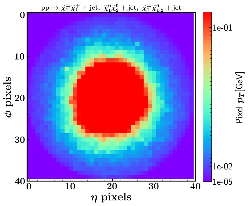
CONTENTS

 I. Introduction                                         3

II. Simulation and Jet Image                             4

III. Neural Network Architecture and Numerical Results   11

IV. Conclusion                                           16

V. Acknowledgements                                      16

   References                                            16

                                         2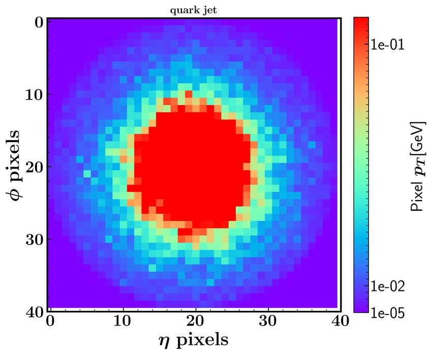
I.    INTRODUCTION

     The existence of dark matter (DM) has been verified in various astrophysics and cosmo-
logical observations. One of the attractive candidates for the DM particle is the Weakly-
Interacting Massive Particles (WIMPs). When the R-parity is conserving, the lightest neu-
        e01 in the supersymmetric models can naturally play the role of WIMP dark matter [1].
tralino χ
     e01 is higgsino-like and light, its annihilation rate is usually too large to saturate the
When χ
thermal relic density of DM [2]. Thus, other production mechanisms, such as non-thermally
produced DM, are needed [3]. The phenomenology of light higgsino DM has been studied
in Refs. [4–24].

     On the other hand, in the supersymmetric models, the naturalness strongly indicates
that the higgsinos mass should not be far above the weak scale [25–28]. Searching for
the light higgsino particles is a key test of the supersymmetric naturalness criteria. When
                                    e±
µ  M1 , M2 , the lightest chargino χ                                   e01 , χ
                                     1 and the two lightest neutralinos χ     e02 will be higgsino-
like. The strategies of probing these new light particles at colliders are sensitive to the mass
difference ∆M between the LSP and NLSP. The conventional methods of searching for
the electroweakinos require the hard leptons in the final states. But if ∆M is small, the
decay products of the electroweakinos would become soft. In the past, several new ways
of accessing such a compressed spectrum have been proposed at colliders [29–36]. Among
them, the mono-jet signature was used to probe the nearly degenerate higgsinos at the LHC.
Due to the large systematics, the additional isolated soft leptons in the final states may help
to improve the sensitivity. However, when the mass splitting is small enough, such leptons
would fail to reach the lepton triggers in the LHC experiments [37, 38].

     In recent years, machine learning (ML) has been widely used in the fields of particle
collision data processing and classification (see recent reviews, e.g. [39–44]). In contrast
with the traditional cut-based analysis, ML provides a new way to optimize the signal-to-
noise ratios. In Refs. [45, 46], it is found that the four-momentum information of the particles
inside the jets can be converted into a two-dimensional (2D) image. To deal with the jet
images, the convolutional neural network (CNN) and its variants have been often adopted
in the analyses [47–58]. For example, in Ref. [51], they studied the image-based networks
to distinguish hadronically decaying top quarks from a background of light quark or gluon
jets. In Ref. [52], the different neural network classifiers are trained to distinguish between

                                               3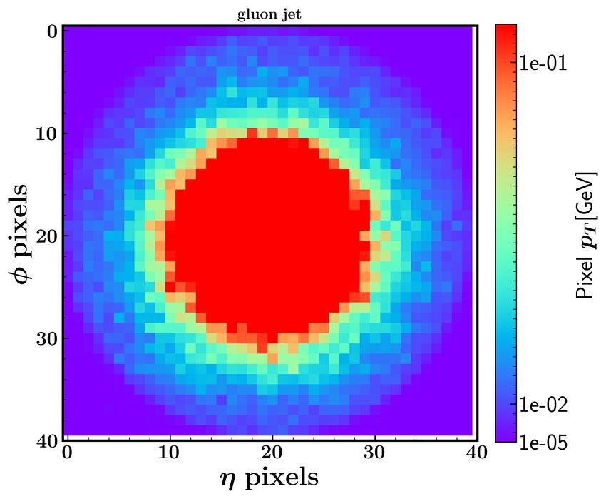
quark/gluon-initiated jets. By using the multi-channel CNNs, their results can be better
than that using the boosted decision tree (BDT). In Ref. [55], they use Lund jet plane images
data to train CNNs to distinguish hadronically decaying Higgs from the QCD backgrounds.
By comparing the cut-based approach with the jet color ring observable, they found that the
CNN method can give a higher tagging efficiency for all the cases. In Ref. [56], the authors
apply the CNN algorithm to study the photon-jet events from the light axion-like particles
and obtain a stronger bound on the axion-photon couplings in the MeV-GeV mass range.
      In this work, we will utilize the deep learning jet image method to search for the light
nearly-degenerate higgsino DM from the monojet events at the LHC. We note that the lead-
                                                                        e±
ing jets from the initial state radiations in our signal processes pp → χ1χe∓    e01 χ
                                                                            1 j, χ          e±
                                                                                     e02 j, χ1χe01,2 j
contain more gluon jets than the main backgrounds Z/W +jets, while the latter are almost
entirely dominated by the quark jets, which have different patterns in the jet images. This
feature can be used as a handle to improve the signal sensitivity. Also we will compare
our method with the conventional cut-based analysis. The paper is organized as follows:
In Sec. II, we present the simulation of signal and background events and construct the jet
image. In Sec. III, we describe the neural network architecture in our analysis and discuss
the numerical results. Finally, we draw the conclusions in Sec. IV.

II.     SIMULATION AND JET IMAGE

                  FIG. 1. Feynman diagrams of our signal processes on the LHC.

      In our simplified nearly-degenerate higgsino scenario, the monojet events are from the
               e±
processes pp → χ1χe∓    e01 χ
                   1 j, χ          e±
                            e02 j, χ  e01,2 j, whose Feynman diagrams are shown in Fig. 1. Since
                                     1χ

µ  M1 , M2 , the production cross sections of the signal events are sensitive to the higgsino
mass parameter µ but almost independent of the value of tan β. The dominant SM back-
grounds we consider are Z(→ ν ν̄) + jets, W ± (→ lν) + jet, and W ± (→ τ ± ν) + jet. We ignore

                                                 4
tt̄ background because its contribution to the sensitivity is much smaller than others [29]. In
this paper we will explore the potential of using the CNN to identify 2D image information
of the monojet to distinguish our signal from the backgrounds.
We use SUSY-HIT [59] to calculate the mass spectrum of the relevant sparticles. The
parton level signal and backgrounds are generated by MadGraph5 aMC@NLO [60]. The
parton shower and hadronization are performed with Pythia-8 [61]. The detector simulation
is carried out by Delphes [62]. In Delphes, the electromagnetic calorimeter (ECAL) measures
the energy of electrons and photons. All the energies of electrons and photons are deposited
in the ECAL by default. The hadron calorimeter (HCAL) measures the energy of long-lived
charged and neutral hadrons. Although a fraction of the energy of stable hadrons would be
deposited in the ECAL in the realistic detectors, it is assumed that all energy of the hadrons
is deposited in the HCAL in the Delphes. Kaons and Λ are considered long-lived by most
detectors. In Delphes, their energies are assumed to be distributed in the ECAL and HCAL
at fECAL = 0.3 and fHCAL = 0.7 [62]. For the reasonable statistics, we imposed a parton-level
cut of pT > 120 GeV and |η| < 5 on the leading jet when generating the parton-level signal
and background events. Finally, with the particle-flow algorithm [62–64], the EflowPhotons,
the EflowNeutralHadrons, and the ChargedHadrons, consist of the energy deposits in the
ECAL and HCAL. They are clustered into jets by FastJet [65] by using the anti-kt algorithm
with Rj = 0.7 [66].
The particles inside the monojet usually contain the useful information, such as the
transverse momentum Ptx , the pseudorapidity η, and the azimuthal angle φ of each parti-
0 00
cle, the transverse momentum Ptx of each photon, the transverse momentum Ptx of each
000
uncharged hadron, and the transverse momentum Ptx of each charged hadron. We perform
the principal component analysis (PCA) on the six-dimensional original variables and plot
the histograms of the variance of the new eigenvectors in Fig. 2. In the PCA, a set of possi-
bly correlated variables is transformed into a set of linearly independent variables through
the orthogonal transformation, where the transformed set of variables is called the principal
components [67–70]. In a nutshell, the PCA is a dimensionality reduction method that uses
fewer data to represent more salient features. The six new principal component variables
given by the PCA are shown in Fig. 2. All these components are the linear combinations of
the original variables described above. When we use the linear combination of the original
0
variable with maximum variance, the principal components (dimension is M ) can effec-
5FIG. 2. The variance of each principal component after principal component analysis (PCA) of the
substructure information of monojet in the signal and background. The component with a large
variance contains more characteristic information.
tively represent the characteristics of the original variables (dimension is M ). In this paper,
0
M < M = 6. From Fig. 2, we can find that the variance of the first principal component is
the largest, and represents the direction of the largest variance in the variable.
In Fig. 3, we plot the distributions of the cumulative variance contribution ratio Rc of
the new feature variables for the signal and backgrounds. From Fig. 3, we can find that the
values of Rc of the first two principal components have reached about 85%, while the values
of Rc of the first three principal components are almost higher than 99%. Therefore, two
or three principal component variables with large variances are sufficient to represent the
6FIG. 3. The cumulative variance contribution rate (Rc ) of the principal components. The cumu-
lative variance contribution of six new eigenvariables is equal to one.
variable features of our study.
By comparing the original features and the new principal component axis, we can find out
which features play the important role in holding information. We expect the classification
performance will be improved by using the principal components as the new feature variables.
On the other hand, in our study, to determine features that are most relevant for the
2D analysis, we choose to use the original feature variables, which include the transverse
momentum Ptx , the pseudorapidity η, and the azimuthal angle φ of each particle [69]. At
the same time, these three original variables can be easily used to construct the jet images.
In Fig. 4, we show the normalized distributions of the leading jet pT (j1 ) and the missing
7/ T . It can be seen that the transverse momentum of the leading jet in
transverse energy E
/ T in the signal drops more
the signal is harder than that in the background, and the E
slowly than that in the background. Thus, we choose pT (j1 ) > 300 GeV and |ηj1 | < 2, and
/ T > 300 GeV to effectively reduce the background [21]. For statistics, we also keep the
E
second jet with pT (j2 ) < 100 GeV and |ηj2 | > 2 in our analysis. At the same time, we veto
the events with more than two jets with pT greater than 30 GeV in the area of |η| < 4.5. On
the other hand, we veto the events with an identified lepton(l = e, µ, τ ) and b-jet to reduce
/ T ) > 0.7 to reduce most
the backgrounds. In addition, we use the requirements of ∆φ(j1 , E
of the QCD backgrounds [71, 72]. The basic selections of the signal and background events
are shown in Tab. I. After the basic cuts, we will train the samples with the CNN.
/ T of the signal and
FIG. 4. The normalized distributions of the leading jet pT (j1 ) and the E
background events at the 14 TeV LHC.
To construct the jet images, we use the transverse momentum Ptx , the pseudorapidity η
and the azimuthal angle φ of each particle in the original variables. We integrate the jet
composition information provided by ECAL and HCAL into digital images [46]. The jet
image is a 40 × 40 square grid, which is centered around the leading jet with the radius
Rj = 0.7. The pixel of each grid in the plane of (∆η, ∆φ) corresponds to the sum of the
transverse momentum of each particle falling in the grid [73].
We pre-process all jet images by using translation, rotation, and normalization. The
purpose of pre-processing is to make the CNN learn more about the essential information
about the signal and backgrounds. In the translation, we move the center of the jet image
8Basic Cuts Z(ν ν̄)+j W ± (lνl )+j W ± (τ ± ντ )+j signal(µ =100 GeV) signal(µ = 200 GeV)
pT (j1 ) > 300 GeV
10348 9863 9908 27544 43810
|ηj1 | < 2
/ T > 300 GeV
E 6549 1804 3122 19999 35307
pT (j2 ) < 100 GeV
|ηj1 | > 2 1531 385 478 3787 7203
pT (j3 ) < 30 GeV
veto on e,µ, τ 1507 179 323 3686 7080
veto on b-jet 1455 177 319 3558 6839
/ T ) > 0.7
∆φ(j1 , E 1452 175 316 3536 6799
TABLE I. The basic cut flows of the cross sections (in units of pb) of the signal and backgrounds
at 14 TeV LHC. The higgsino mass µ = 100, 200 are taken in the calculations
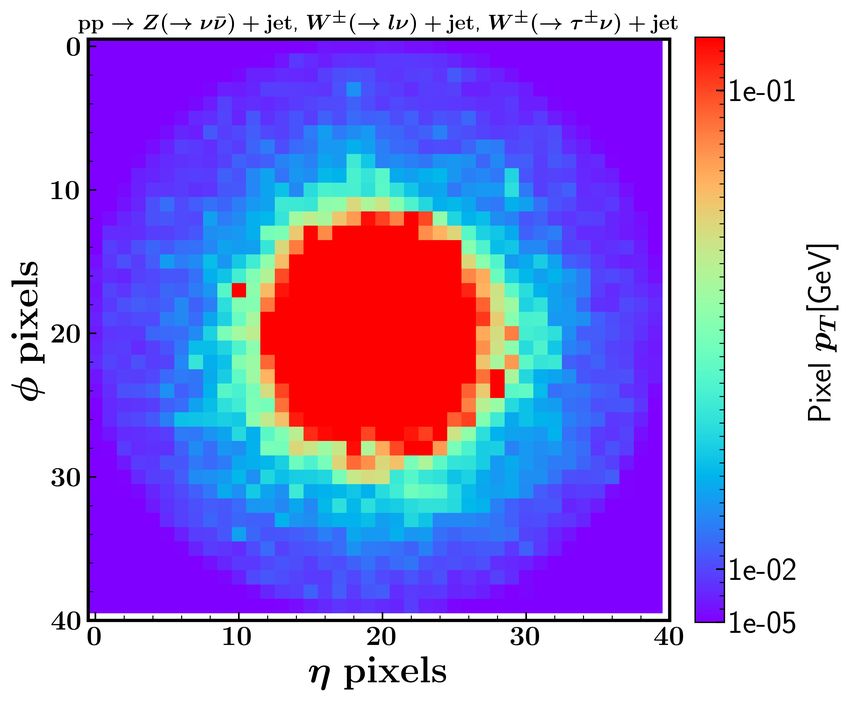
FIG. 5. The jet images of the leading jet in the total backgrounds (left panel) and signal (right
panel) after the translation and rotation. The higgsino mass is taken as µ = 200 GeV.
0 0
(η 0 , φ0 ) to the origin of our new coordinate system (η , φ ) as,
η i0 = η i − η 0 , φi0 = φi − φ0 , (1)
where the index i is the number of each pixel. We define the “center of mass” of a jet image
9as,
n n
1 X i0 1 X i0
ηc = P η pTi , φc = P φ pTi , (2)
i pTi i=1 i pTi i=1
Then, we can rotate it of each jet image to the vertical axis around its center as,
η i00 = η i0 cos α − φi0 sin α, φi00 = φi0 cos α + η i0 sin α, (3)
with
ηc φc
cos α = p , sin α = p . (4)
ηc2 + φ2c ηc2 + φ2c
After the translation and rotation, we convert the transverse momentum of the particles
into pixel values of the 2D image as,
n
X
Pij = Pa , (i, j ∈ [1, 40]),
a=1 (5)
i00
η + 0.7 φi00 + 0.7
i= , j= ,
0.035 0.035
where n is the number of particles inside the specific grid in each event whose pseudorapidity
and azimuthal angle is equal to (η i , φi ). In Fig. 5, we show the jet images of the signal and
total backgrounds after the translation and rotation, where the pixel value in each grid is
the sum average of the transverse momentum P = Ptx of the particles inside the jet in each
event falling in the corresponding grid. In order to reach higher efficiency in the analysis,
we normalize the transverse momentum of the particles within each jet as
pTi − min(pT )
yi = . (6)
max(pT ) − min(pT )
where yi takes the values in the range of [0,1].
From Fig. 6, we can see that the pixel area of the gluon jets is larger than that of the quark
jets. This can be understood that the quark jets carry only one quantum chromodynamic
(QCD) color, while the gluon jet has both color and inverse color. Theoretically, the Altarelli-
Parisi splitting function [74] contains a factor CA = 3 for the gluon radiation from the gluons
4
and a factor CF = 3
for the gluon radiation from the quarks. Therefore, the gluon jets tend
to have more composition and broader pixel area in the η-φ plane than the quark jets [52, 75].
In our calculation, we find that the gluon leading jet in the signal accounts for about 40%,
while its proportion in the background is about 16%. Thus, the leading jets in the signal
events tend to have broader pixel area than those in the background events.
10FIG. 6. The jet images of the quark jet (left panel) and the gluon jet (right panel) in the signal
after the translation and rotation. The higgsino mass is taken as µ = 200 GeV.
III. NEURAL NETWORK ARCHITECTURE AND NUMERICAL RESULTS
We design a convolutional neural network (CNN) within the deep learning framework of
PyTorch [76]. We use the GPU to accelerate the training of the classifier. In the CNN,
we use the convolution kernel to extract the features of the input image and the activation
function to increase the expression ability of the model. Then we employ the maximum
pooling layer to reduce the dimensionality of the network to accelerate the training process.
After that, we use the gradient descent method to find the minimum loss function value, and
finally, adopt the fully connected layer for classification. The first three steps above realize
the mapping of the original data to the hidden layer feature space, and the last step is to
map the learned feature distribution to the sample label space for classification prediction.
As shown in Fig. 7, the input 2D image pixels are 40 × 40 with one channel. The number
of convolution kernels is 32, the size is 5 × 5, and the stride is two. Before the convolution
operation, we add two layers of zero at the periphery of the input image to fully extract
the edge information of the image and make the image maintains the same dimensions
after convolution. Then, we use a non-linear activation function to increase the expressive
power of the model. Since both the Sigmoid-type function and the tanh(x)-type function
have gradient saturation effects, and the ReLU function has a “dead zone”, the above three
methods are not conducive to gradient convergence. Thus, we choose the Leaky ReLU
11function here and find that it is indeed better than the above three activation functions.
In order to reduce the number of parameters and speed up the operation, we use grouped
convolution so that the convolutional kernels in each group are convoluted with only one
feature map.
In order to decrease the sensitivity of the network to the absolute location of elements
in the image and reduce parameters, we apply a stack of 2 × 2 maxpooling layers to obtain
the 20 × 20 feature maps with 32 channels. Next, we repeat the above process to obtain
the 5 × 5 feature maps of 128 channels. Whereafter, we flatten the final feature map to
a single vector and apply two fully connected layers with 128 and 32 neurons respectively.
Finally, we apply the softmax activation function to output the probabilities of the signal
and background.
eSi
s = PC (i = 1, 2, 3, ......N ), (7)
Sij
j=1 e
where N is the total number of the samples. C refers to the number of categories and is
taken as C=2 in our study. The softmax function s allows the output values of a multiclass
to be converted into a probability distribution with a sum of one in the range of [0, 1]. The
network architecture we use is shown in the Fig. 7.
In addition to the above feedforward operation, a complete machine learning network
also needs feedback operation to adjust network parameters and optimize the classification
accuracy of the model. In our feedback operation, we define the cross-entropy loss function
L to calculate the loss rate,
N
1 X
L= (yi0 log pi0 + yi1 log pi1 ). (8)
N i=1
where N is the number of samples, yi0,i1 and pi0,i1 are the true and predicted category of the
signal and background samples, respectively. We take the Adam optimizer with a learning
rate of 0.001 [77].
In the left panel of Fig. 8, the dependence of the loss function of the training set and the
validation set on the epoch is shown. The data set of training and validation contains 400k
events, respectively. During the training, the minimum batch of input data is 1024 event
samples, and the maximum epoch is set to 100. After the end of the first epoch, each event in
the training set is used once. In order to avoid learning the distribution order characteristics
of the cases, we randomly scramble the order of the data before each new epoch starts.
12FIG. 7. The architecture of our convolutional neural network.
We also use the same amount of signal and background events as the validation set. We
find that the validation set loss function value reaches the minimum as the training reaches
about the 43rd epoch. After this epoch, the classifier will learn more detailed features in
the training data and then results in over-fitting. Since then, the recognition efficiency of
the data in the training set became higher and higher, however, the recognition efficiency of
the new batch of validation set data became worse and worse. We stop the training at the
43rd epoch. Therefore, we choose the classifier with the smallest loss function value in the
validation data set as our best classifier.
In the right panel of Fig. 8, we show the test set classification effect for the signal and
background events after training the CNN, where s denotes the probability that a sample
will be determined as a signal sample after passing through the classifier. The area under the
red and blue lines represent the probability density distribution of the signal and background
samples, respectively. The former is very close to one, while the latter is very close to zero.
13However, the irreducible background pp → Z(→ ν ν̄) + jet can contribute a small portion in
the region of s ∼ 1.
FIG. 8. The dependence of the loss function on the epoch for training samples and validation
samples (left panel); The classification effect diagram of the test set of signals and backgrounds
(right panel).
In the left panel of Fig. 9, we show the receiver operating characteristic (ROC) curves
and the corresponding values of the area under curve (AUC), where µ = 100, 160, 200 GeV.
The true positive rate (εS ) and false positive rate (εB ) represent the fraction of the survival
events in the initial signal and background events, respectively. The ROC curves can be
obtained from the probability density distribution in the right panel of Fig. 8. If choosing the
cut value s0 , we can use the respective probability densities of the signal and background in
the s > s0 region as the function values in the ROC curve. When the AUC value approaches
one, the classification effect of the classifier is better.
To obtain the observability of the signal, we assume the Poisson distribution to calculate
the signal significance Z,
S
Z=p , (9)
B + (βB)2
where S and B denote the number of the signal and background events after all cuts,
respectively. We require the signal events larger than 20 to ensure the statistics and estimate
the contribution of the systematic error as βB. In comparison with the previous results based
14on the cut-flow in Ref. [29], we also focus on the same mass range of [100, 200] GeV and
calculate the significance with the same value of β = 1% at 14 TeV LHC with the integrated
luminosity of 3000 fb−1 . To show the improvement, we define the significance ratio of the
CNN result Zcnn to the cut-based result Zcut−based as,
Zcnn
Rs = (10)
Zcut−based
From Fig. 9, we can see that the image recognition technology using the CNN can greatly
improve the traditional cut-based results by a factor of two in the low mass range. As
the higgsino mass increases, the improvement will decrease because the production cross
section of the signal process becomes small. Therefore, when the light higgsinos are highly-
degenerate and the soft leptons cannot be used as triggers, the monojet signal will play an
important role in searching for these light higgsinos. The application of deep learning jet
image may be able to effectively enhance the sensitivity of probing the light nearly-degenerate
higgsinos from the mono-jet events at the HL-LHC.
FIG. 9. The ROC curves and the corresponding AUC values (left panel). The significance ratio
Rs of the CNN result Zcnn to the cut-based result Zcut−based (right panel) at the HL-LHC.
15IV. CONCLUSION
In this paper, we study the search of the light higgsino dark matter within the natural
MSSM at 14 TeV-LHC with 3000 f b−1 luminosity. The production processes of our signal
e±
are mainly pp → χ1χe∓ e01 χ
1 +jet, χ e±
e02 +jet, χ1χe01,2 +jet. We convert the information of a jet into
a 2D jet image and use the CNN to deeply learn the signal and background image features
to enhance the signal observability. Our numerical calculation shows that the sensitivity
based on CNN can be about [1.6, 2.2] times as large as that based on the cut-flow method.
V. ACKNOWLEDGEMENTS
We thank Yuchao Gu, Song Li, and Jie Ren for their helpful discussions. In addition,
we would like to thank Prof. Jin Min Yang for his warm hospitality at the Institute of
Theoretical Physics. This work is supported by the National Natural Science Foundation of
China (NNSFC) under grant 12147228.
[1] G. Jungman, M. Kamionkowski, and K. Griest, Phys. Rept. 267, 195 (1996), arXiv:hep-
ph/9506380.
[2] N. Arkani-Hamed, A. Delgado, and G. F. Giudice, Nucl. Phys. B 741, 108 (2006), arXiv:hep-
ph/0601041.
[3] H. Baer, K.-Y. Choi, J. E. Kim, and L. Roszkowski, Phys. Rept. 555, 1 (2015),
arXiv:1407.0017 [hep-ph].
[4] G. F. Giudice and A. Pomarol, Phys. Lett. B 372, 253 (1996), arXiv:hep-ph/9512337.
[5] K. Freese and M. Kamionkowski, Phys. Rev. D 55, 1771 (1997), arXiv:hep-ph/9609370.
[6] J. L. Feng, K. T. Matchev, and F. Wilczek, Phys. Lett. B 482, 388 (2000), arXiv:hep-
ph/0004043.
[7] G. F. Giudice, T. Han, K. Wang, and L.-T. Wang, Phys. Rev. D 81, 115011 (2010),
arXiv:1004.4902 [hep-ph].
[8] H. Baer, V. Barger, and P. Huang, JHEP 11, 031 (2011), arXiv:1107.5581 [hep-ph].
[9] J. Cao, C. Han, L. Wu, J. M. Yang, and Y. Zhang, JHEP 11, 039 (2012), arXiv:1206.3865
[hep-ph].
16[10] H. Baer, V. Barger, and D. Mickelson, Phys. Lett. B 726, 330 (2013), arXiv:1303.3816 [hep-
ph].
[11] K. Kowalska and E. M. Sessolo, Phys. Rev. D 88, 075001 (2013), arXiv:1307.5790 [hep-ph].
[12] C. Han, K.-i. Hikasa, L. Wu, J. M. Yang, and Y. Zhang, JHEP 10, 216 (2013), arXiv:1308.5307
[hep-ph].
[13] J. Cao, C. Han, L. Wu, P. Wu, and J. M. Yang, JHEP 05, 056 (2014), arXiv:1311.0678
[hep-ph].
[14] M. Low and L.-T. Wang, JHEP 08, 161 (2014), arXiv:1404.0682 [hep-ph].
[15] N. Nagata and S. Shirai, JHEP 01, 029 (2015), arXiv:1410.4549 [hep-ph].
[16] D. Barducci, A. Belyaev, A. K. M. Bharucha, W. Porod, and V. Sanz, JHEP 07, 066 (2015),
arXiv:1504.02472 [hep-ph].
[17] L. Aparicio, M. Cicoli, B. Dutta, F. Muia, and F. Quevedo, JHEP 11, 038 (2016),
arXiv:1607.00004 [hep-ph].
[18] N. Liu and L. Wu, Eur. Phys. J. C 77, 868 (2017), arXiv:1705.02534 [hep-ph].
[19] M. Abdughani, L. Wu, and J. M. Yang, Eur. Phys. J. C 78, 4 (2018), arXiv:1705.09164
[hep-ph].
[20] C. Han, R. Li, R.-Q. Pan, and K. Wang, Phys. Rev. D 98, 115003 (2018), arXiv:1802.03679
[hep-ph].
[21] M. Abdughani and L. Wu, Eur. Phys. J. C 80, 233 (2020), arXiv:1908.11350 [hep-ph].
[22] H. Baer, V. Barger, S. Salam, D. Sengupta, and X. Tata, Phys. Lett. B 810, 135777 (2020),
arXiv:2007.09252 [hep-ph].
[23] A. Delgado and M. Quirós, Phys. Rev. D 103, 015024 (2021), arXiv:2008.00954 [hep-ph].
[24] J. Dai, T. Liu, D. Wang, and J. M. Yang, (2022), arXiv:2202.03258 [hep-ph].
[25] J. L. Feng, K. T. Matchev, and T. Moroi, Phys. Rev. Lett. 84, 2322 (2000), arXiv:hep-
ph/9908309.
[26] J. L. Feng, K. T. Matchev, and T. Moroi, Phys. Rev. D 61, 075005 (2000), arXiv:hep-
ph/9909334.
[27] M. Papucci, J. T. Ruderman, and A. Weiler, JHEP 09, 035 (2012), arXiv:1110.6926 [hep-ph].
[28] L. J. Hall, D. Pinner, and J. T. Ruderman, JHEP 04, 131 (2012), arXiv:1112.2703 [hep-ph].
[29] C. Han, A. Kobakhidze, N. Liu, A. Saavedra, L. Wu, and J. M. Yang, JHEP 02, 049 (2014),
arXiv:1310.4274 [hep-ph].
17[30] A. Arbey, M. Battaglia, and F. Mahmoudi, Phys. Rev. D 89, 077701 (2014), arXiv:1311.7641
[hep-ph].
[31] Z. Han, G. D. Kribs, A. Martin, and A. Menon, Phys. Rev. D 89, 075007 (2014),
arXiv:1401.1235 [hep-ph].
[32] P. Schwaller and J. Zurita, JHEP 03, 060 (2014), arXiv:1312.7350 [hep-ph].
[33] C. Han, D. Kim, S. Munir, and M. Park, JHEP 04, 132 (2015), arXiv:1502.03734 [hep-ph].
[34] M. Abdughani, J. Ren, L. Wu, and J. M. Yang, JHEP 08, 055 (2019), arXiv:1807.09088
[hep-ph].
[35] H. Fukuda, N. Nagata, H. Oide, H. Otono, and S. Shirai, Phys. Rev. Lett. 124, 101801 (2020),
arXiv:1910.08065 [hep-ph].
[36] H. Baer, V. Barger, D. Sengupta, and X. Tata, (2021), arXiv:2109.14030 [hep-ph].
[37] G. Aad et al. (ATLAS), Eur. Phys. J. C 81, 1118 (2021), arXiv:2106.01676 [hep-ex].
[38] A. Tumasyan et al. (CMS), (2021), arXiv:2111.06296 [hep-ex].
[39] J. Ren, L. Wu, J. M. Yang, and J. Zhao, Nucl. Phys. B 943, 114613 (2019), arXiv:1708.06615
[hep-ph].
[40] D. Guest, K. Cranmer, and D. Whiteson, Ann. Rev. Nucl. Part. Sci. 68, 161 (2018),
arXiv:1806.11484 [hep-ex].
[41] K. Albertsson et al., J. Phys. Conf. Ser. 1085, 022008 (2018), arXiv:1807.02876 [physics.comp-
ph].
[42] M. Abdughani, J. Ren, L. Wu, J. M. Yang, and J. Zhao, Commun. Theor. Phys. 71, 955
(2019), arXiv:1905.06047 [hep-ph].
[43] M. Feickert and B. Nachman, (2021), arXiv:2102.02770 [hep-ph].
[44] G. Karagiorgi, G. Kasieczka, S. Kravitz, B. Nachman, and D. Shih, (2021), arXiv:2112.03769
[hep-ph].
[45] J. Cogan, M. Kagan, E. Strauss, and A. Schwarztman, JHEP 02, 118 (2015), arXiv:1407.5675
[hep-ph].
[46] L. de Oliveira, M. Kagan, L. Mackey, B. Nachman, and A. Schwartzman, JHEP 07, 069
(2016), arXiv:1511.05190 [hep-ph].
[47] A. Aurisano, A. Radovic, D. Rocco, A. Himmel, M. D. Messier, E. Niner, G. Pawloski, F. Psi-
has, A. Sousa, and P. Vahle, JINST 11, P09001 (2016), arXiv:1604.01444 [hep-ex].
18[48] P. T. Komiske, E. M. Metodiev, and M. D. Schwartz, JHEP 01, 110 (2017), arXiv:1612.01551
[hep-ph].
[49] J. Guo, J. Li, T. Li, F. Xu, and W. Zhang, Phys. Rev. D 98, 076017 (2018), arXiv:1805.10730
[hep-ph].
[50] J. Lin, M. Freytsis, I. Moult, and B. Nachman, JHEP 10, 101 (2018), arXiv:1807.10768
[hep-ph].
[51] A. Butter et al., SciPost Phys. 7, 014 (2019), arXiv:1902.09914 [hep-ph].
[52] J. S. H. Lee, I. Park, I. J. Watson, and S. Yang, J. Korean Phys. Soc. 74, 219 (2019),
arXiv:2012.02531 [hep-ex].
[53] J. Guo, J. Li, T. Li, and R. Zhang, Phys. Rev. D 103, 116025 (2021), arXiv:2010.05464
[hep-ph].
[54] M. Abdughani, D. Wang, L. Wu, J. M. Yang, and J. Zhao, Phys. Rev. D 104, 056003 (2021),
arXiv:2005.11086 [hep-ph].
[55] C. K. Khosa and S. Marzani, Phys. Rev. D 104, 055043 (2021), arXiv:2105.03989 [hep-ph].
[56] J. Ren, D. Wang, L. Wu, J. M. Yang, and M. Zhang, JHEP 11, 138 (2021), arXiv:2106.07018
[hep-ph].
[57] S. Jung, Z. Liu, L.-T. Wang, and K.-P. Xie, Phys. Rev. D 105, 035008 (2022),
arXiv:2109.03294 [hep-ph].
[58] S. Chigusa, S. Li, Y. Nakai, W. Zhang, Y. Zhang, and J. Zheng, (2022), arXiv:2202.02534
[hep-ph].
[59] A. Djouadi, M. M. Muhlleitner, and M. Spira, Acta Phys. Polon. B 38, 635 (2007), arXiv:hep-
ph/0609292.
[60] J. Alwall, R. Frederix, S. Frixione, V. Hirschi, F. Maltoni, O. Mattelaer, H. S. Shao, T. Stelzer,
P. Torrielli, and M. Zaro, JHEP 07, 079 (2014), arXiv:1405.0301 [hep-ph].
[61] T. Sjöstrand, S. Ask, J. R. Christiansen, R. Corke, N. Desai, P. Ilten, S. Mrenna, S. Pres-
tel, C. O. Rasmussen, and P. Z. Skands, Comput. Phys. Commun. 191, 159 (2015),
arXiv:1410.3012 [hep-ph].
[62] J. de Favereau, C. Delaere, P. Demin, A. Giammanco, V. Lemaı̂tre, A. Mertens, and M. Sel-
vaggi (DELPHES 3), JHEP 02, 057 (2014), arXiv:1307.6346 [hep-ex].
[63] M. Aaboud et al. (ATLAS), Eur. Phys. J. C 77, 466 (2017), arXiv:1703.10485 [hep-ex].
[64] A. M. Sirunyan et al. (CMS), JINST 12, P10003 (2017), arXiv:1706.04965 [physics.ins-det].
19[65] M. Cacciari, G. P. Salam, and G. Soyez, Eur. Phys. J. C 72, 1896 (2012), arXiv:1111.6097
[hep-ph].
[66] M. Cacciari, G. P. Salam, and G. Soyez, JHEP 04, 063 (2008), arXiv:0802.1189 [hep-ph].
[67] O. Lahav, Vistas Astron. 38, 251 (1994), arXiv:astro-ph/9411071.
[68] S. Adanti, P. Battinelli, R. Capuzzo-Dolcetta, and P. W. Hodge, Astron. Astrophys. Suppl.
Ser. 108, 395 (1994), arXiv:astro-ph/9406027.
[69] C. K. Khosa, V. Sanz, and M. Soughton, SciPost Phys. 10, 151 (2021), arXiv:1910.06058
[hep-ph].
[70] Y. Uchiyama and K. Nakagawa, “Schrödinger risk diversification portfolio,” (2022),
arXiv:2202.09939 [q-fin.PM].
[71] A. M. Sirunyan et al. (CMS), JHEP 08, 016 (2018), arXiv:1804.07321 [hep-ex].
[72] F. Jorge, R. Ronald, S. Jesus, M. Juan, and A. Carlos, (2021), arXiv:2106.06813 [hep-ph].
[73] P. T. Komiske, E. M. Metodiev, B. Nachman, and M. D. Schwartz, J. Phys. Conf. Ser. 1085,
042010 (2018).
[74] G. Altarelli and G. Parisi, Nucl. Phys. B 126, 298 (1977).
[75] (2017).
[76] A. Paszke, S. Gross, F. Massa, A. Lerer, J. Bradbury, G. Chanan, T. Killeen, Z. Lin,
N. Gimelshein, L. Antiga, A. Desmaison, A. Kopf, E. Yang, Z. DeVito, M. Raison, A. Tejani,
S. Chilamkurthy, B. Steiner, L. Fang, J. Bai, and S. Chintala, in Advances in Neural In-
formation Processing Systems, Vol. 32, edited by H. Wallach, H. Larochelle, A. Beygelzimer,
F. d'Alché-Buc, E. Fox, and R. Garnett (Curran Associates, Inc., 2019).
[77] D. P. Kingma and J. Ba, (2014), arXiv:1412.6980 [cs.LG].
20You can also read