CORAL: Colored structural representation for bi-modal place recognition
←
→
Page content transcription
If your browser does not render page correctly, please read the page content below
CORAL: Colored structural representation for
                                                                        bi-modal place recognition
                                                             Yiyuan Pan, Xuecheng Xu, Weijie Li, Yunxiang Cui, Yue Wang, Rong Xiong

                                             Abstract— Place recognition is indispensable for a drift-free
                                         localization system. Due to the variations of the environment,
                                         place recognition using single-modality has limitations. In this
                                         paper, we propose a bi-modal place recognition method, which
                                         can extract a compound global descriptor from the two modal-
                                         ities, vision and LiDAR. Specifically, we first build the elevation
arXiv:2011.10934v2 [cs.CV] 19 Jul 2021

                                         image generated from 3D points as a structural representation.
                                         Then, we derive the correspondences between 3D points and
                                         image pixels that are further used in merging the pixel-wise
                                         visual features into the elevation map grids. In this way, we
                                         fuse the structural features and visual features in the consistent
                                         bird-eye view frame, yielding a semantic representation, namely
                                         CORAL. And the whole network is called CORAL-VLAD.
                                         Comparisons on the Oxford RobotCar show that CORAL-
                                         VLAD has superior performance against other state-of-the-
                                         art methods. We also demonstrate that our network can be
                                         generalized to other scenes and sensor configurations on cross-
                                         city datasets.
                                                                                                                Fig. 1: The proposed bi-modal coupling of representation
                                                              I. INTRODUCTION                                   fusing visual image and elevation image retrieves the most
                                                                                                                similar sample in the reference maps with different environ-
                                            Loop closure is essential for the localization system be-           mental conditions, like (a) overcast, (b) sun, (c) night, and
                                         cause of the drift reduction, especially in large-scale outdoor        (d) dawn.
                                         scenes. A popular pipeline for loop closure usually employs
                                         place recognition as the first step, since it is able to find a
                                         place from the large map database that is close to the current         LiDAR-based place recognition methods employ deep neural
                                         place, based on purely sensor data similarity. Therefore,              networks to extract structural features from LiDAR scans
                                         place recognition is widely applied in various autonomous              [13, 1], demonstrating superior performance than the visual
                                         robot systems for navigation.                                          place recognition, especially in changing outdoor environ-
                                            The camera is the most popular sensor as it observes                ment. However, LiDAR still has its weakness when the
                                         the texture of the environment at a low cost. Therefore,               environmental structure has fewer features.
                                         visual place recognition draws research attention for years. A            Due to the inherent shortages of both the camera and
                                         traditional pipeline is to build a global feature descriptor by        LiDAR, it is difficult to extract appropriate features using
                                         aggregating handcrafted sparse local features for each image,          the single-modality sensor to describe numerous complex
                                         e.g. SIFT [14] and SURF [3]. Then the efficient searching              scenes. Thus, multi-sensor data fusion is becoming a feasible
                                         method is used to look for the nearest global descriptor on            solution for place recognition. A common sensor for fusion
                                         the database as the most similar match. With the development           image and geometry information is the RGB-D camera but
                                         of the deep neural network, convolution neural networks                it’s not credible in the outdoor scenes. Using the camera and
                                         (CNNs) demonstrate promising retrieval performance [2, 18,             LiDAR is a more robust way to deal with multi-sensor fusion.
                                         28] by extracting more reliable image descriptors. However,            Whereas, inconsistent viewpoints, diverse observation ranges
                                         due to the susceptibility of the visual image under strong             and data structures of the different sensor data become major
                                         variations of seasons, weather, illumination, and viewpoints,          issues to generate a compound global descriptor effectively.
                                         building robust and discriminative image features remains a            In existing fusion-based place recognition methods, the vi-
                                         challenge.                                                             sual and structural information are processed independently
                                            To relieve the problem, LiDAR has been an alternative               to generate their own descriptors and then concatenated
                                         that provides accurate and relatively stable 3D structural             directly as a compound descriptor without consistency in
                                         information. Following the visual place recognition pipeline,          geometry.
                                                                                                                   In this paper, we set to combine the two modalities,
                                            Yiyuan Pan, Xuecheng Xu, Weijie Li, Yunxiang Cui, Yue Wang,         vision and LiDAR, for place recognition, as shown in Fig.
                                         and Rong Xiong are with the State Key Laboratory of Industrial Con-    1. The main novelty is the construction of the bi-modal
                                         trol Technology and Institute of Cyber-Systems and Control, Zhejiang
                                         University, Zhejiang, China. Yue Wang is the corresponding author      fused representation, namely colored structural representa-
                                         wangyue@iipc.zju.edu.cn.                                               tion (CORAL). As shown in previous works on LiDAR
place recognition, various 3D representations, including            convolution neural networks are used to extract structural
point cloud [1], histogram [32], and polar image [11, 31],          descriptors. Owing to orderless of point clouds, several works
are designed to represent LiDAR scans, which highly impact          convert the raw point clouds into a 3D volume representation,
the efficiency and effectiveness. We propose to build a             such as VoxelNet [34] and volumetric CNNs [23]. However,
local dense elevation map to describe the environmental             the conversion process introduces high quantization loss and
structure. The map also derives the correspondences between         requires lots of computation time. PointNet [22] is a pioneer-
3D points and image pixels. The pixel-wise visual features          ing work that is able to capture structural features from raw
are then inserted into the elevation map grids to semantically      point clouds directly. Combining PointNet and NetVLAD,
‘colorize’ the structural features. With such tightly bi-modal      PointNetVLAD [1] is the first approach to achieve large-scale
coupling, CORAL encodes both visual and structural features         long-term place recognition with the input of raw point data.
in the same consistent bird-eye view (BEV) frame. The               However, PointNet operates each point independently thus
contributions can be summarized as:                                 ignoring the local structure relationship of points. In response
   • A local dense elevation map representation is utilized         to this problem, LPD-Net [13] proposes the adaptive local
     for place recognition, which is irrelevant to LiDAR            feature extraction module and the graph-based neighborhood
     hardware configurations to encode the structural infor-        aggregation module. PCAN [33] introduces an attention map
     mation.                                                        to predict the significance of local regions. Both methods
   • A semantic representation with corresponding geometry          boost the performance of place recognition.
     named CORAL is proposed for place recognition which               Fusion-based place recognition Multi-sensor fusion so-
     is robust towards various environmental changes.               lution by incorporating visual and structural features is a
   • A validation on experiments is conducted to evalu-             more appropriate way to achieve place recognition under
     ate the performance of the proposed method, which              strong environment variations. In recent years, a few fusion-
     shows superior performance in testing and generaliza-          based works have emerged for place recognition. The naive
     tion datasets. The code is also released 1 .                   strategy [30, 19] of generating a compound descriptor from
                                                                    different modality inputs is directly combining two global
                      II. R ELATED W ORK                            descriptors extracted from two independent network streams,
   Vision-based place recognition Vision-based place recog-         ignoring the inner relationship of visual context and geom-
nition is typically regarded as the problem of image retrieval      etry structure in the same region. Referring to some 3D
which is solved by searching the most similar match on the          object detection methods, works of [29, 12] fuse the visual
reference database. Traditionally, some salient image parts         and structural information by operating the intermediate
are encoded as handcrafted local features, such as SURF [3],        structural feature map and visual feature map in the same
SIFT [14], or ORB [16, 17], and then these local features           frame, which inspires us to construct a more discriminative
can be aggregated to a global descriptor leveraging feature         and robust compound descriptor.
aggregated methods, such as Bag-of-visual-words [6], VLAD
                                                                                        III. M ETHODOLOGY
[10] and Fisher Vectors [9]. Obtaining the global descriptor
of a query, efficient searching methods like KD-tree search            The architecture of the proposed fusion network is shown
can be used to look for the closest global descriptor as the        in Fig. 2. The network inputs consist of two streams: raw
most similar match on the reference database. In recent years,      front-view images from the camera and filtered elevation im-
handcrafted local features have been increasingly replaced          ages generated from the LiDAR scans. The two-stream net-
by learnable features using deep neural networks that have          work tightly couples the visual and structural features which
significant improvement in extracting descriptive descriptors.      enforce the final representation to encode the semantics
Several mature networks for extracting local features, like         into the geometric structure. Specifically, the dense elevation
VGG-Net [27] and ResNet [8], achieve an amazing perfor-             image representation encodes the structural information, and
mance on place recognition. As for aggregating local fea-           it also provides the point-to-pixel correspondences, which
tures, inspired by the traditional method - VLAD, NetVLAD           is leveraged to insert visual features into the consistent
[2] is formulated as a learnable function that is better in local   BEV frame. Therefore, aggregating the bi-modal features is
features clustering. Generalized-Mean Pooling [24] is also          geometrically sensible, yielding the final global descriptor
an efficient and differentiable aggregated method, allows the       for place recognition.
network to capture a compact global descriptor in an end-
                                                                    A. Elevation map generation
to-end fashion.
   Structural-based place recognition Considering struc-               We introduce the elevation map representation defined on
tural features are more robust in changing environments,            a grid map. Each 2D grid indexes an elevation to describe the
structural-based methods become an alternative for place            environment structure. Originated in the 2D occupancy grid
recognition. Handcrafted structural descriptors, like PFH [25]      map, the elevation map replaces the occupancy information
and SHOT [26], usually have poor generalizability, that they        with the elevation, which is capable of representing the 2.5D
can only be used in specific tasks. To relieve this problem,        ground surface.
                                                                       First, the 6 degree-of-freedom (DOF) pose of the sensor
  1 https://github.com/Panyiyuan96/CORAL   Pytorch.git              denoted as T is calculated by LiDAR inertial odometry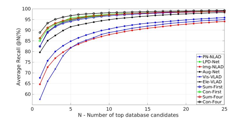
Fig. 2: The network architecture of CORAL-VLAD. The network inputs an elevation image generated by LiDAR scans
and a visual image, and then outputs a global descriptor to predict the most similar scene on the reference database. A
shows multi-scale visual feature map from the output of FPN layer, B shows the BEV visual feature map from the ouput
of projection layer.

algorithm, with respect to the global frame G. Given a     3D
point pi of a new measurement in the sensor frame,         we
transform it into the global frame by T pi and calculate   the
elevation:
                         ep = P T pi                        (1)

the projection matrix P = [0, 0, 1] retrieves 3rd entry of the    Fig. 3: Elevation image generation. The elevation map accu-
transformed point as the elevation ep , while the first two       mulated from raw LiDAR scans is projected on the image
entries are rounded and then converted to the corresponding       plane as a raw elevation image. The filtered elevation image
index of the grid map. For processing multiple observations       is generated using a mean filter.
of the same grid, the variance σp of elevation is introduced to
describe the uncertainty of elevation measurement according       elevation value from 0 to 255 as the grayscale value of the
to range sensor models [5]. In this way, each grid data           elevation image. Additionally, a mean filter is applied to fill
(eg , σg2 ) is updated according to the corresponding measure-    up some invalid pixels which have not been observed on
ment data (ep , σp2 ). Note that only the measurement within      the elevation image using a 3 × 3 filter template. Compared
the Mahalanobis distance threshold of the grid is fused by        with the single scan based BEV representation, the elevation
variance weighted strategy to obtain an updated grid data as      image is much denser to describe the structure, also leading
follows:                                                          to more accurate point-to-pixel correspondences.
                  σp2 eg + σg2 ep             σp2 σg2
           eg =                     σg2 =                   (2)   B. Network architecture
                     σp2 + σg2              σp2 + σg2
                                                                     The architecture of the proposed compound network is
Furthermore, to clear the dynamic objects due to the use          shown in Fig. 2. The whole network can be divided into
of the accumulation mechanism, ray tracing is utilized to         three main components: the feature extraction module, the
check whether the grid is crossed by a ray, and if the grid is    fusion layer, and the local feature aggregation module.
occupied by a dynamic object, the elevation and variance of          Feature extraction Our multi-sensor network has two
this grid are initialized. The detailed generation process can    streams for feature extraction. The visual stream employs
be found in [20].                                                 the lightweight ResNet18 [8] as the backbone to efficiently
   Elevation image To utilize 2D convolution neural net-          extract the visual features. Due to the utilize of several
works directly, the elevation map is converted into a one-        convolutional layers with stride 2, the output feature map
channel grayscale image with the same size as the grid map,       suffers a dramatic reduction in size which is not suitable for
namely elevation image. As shown in Fig. 3, we scale the          fusion. So we use feature pyramid network (FPN) to combine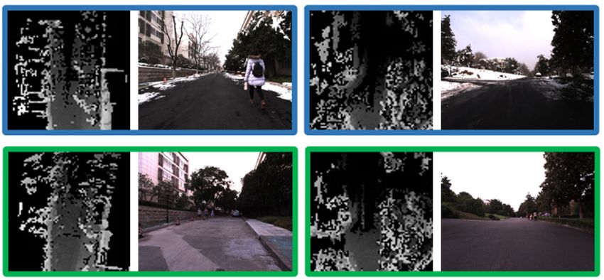
four feature maps from the residual block group to recover         perception (MLP) to process the raw output of NetVLAD
the final feature map with the size same as the first residual     for learning a dimension reduction mapping to decrease the
block and exploit multi-scale feature information.                 size of the global descriptor which accelerates the nearest
   The structural stream comprises a group of convolutional        neighbor search.
layers to capture structural features, and four groups of
residual blocks to extract fusion features. Except for the first   C. Training the fusion descriptor
group, all groups start with the convolution layer with stride
2 and all other convolutions are with stride 1. The number of         We train our compound network in an end-to-end fashion
3 × 3 kernel convolutions in each group is 2, 4, 4, 6, 6, and      to yield a bi-modal fused global descriptor. A margin-based
each group outputs the feature vector with the corresponding       loss is adopted to train pairs of samples labeled with positive
dimensions of 64, 64, 128, 192, and 256 respectively. The          or negative based on corresponding GPS position.
outputs of the last three residual blocks also exploit multi-         Loss function The training data is constructed as sets
scale information as the visual stream does.                       of tuples T = (Pa , {Ppos } , {Pneg }). Pa denotes an
   Fusion Layer The fusion layer comprises two compo-              anchor with a pair of visual image and elevation im-
nents: the projection layer and the fusion module. The goal of     age, {Ppos } , {Pneg } represent the set of anchor’s positive
the projection layer is to convert the front-view visual feature   matches and negative matches determined by the their rel-
map into the BEV visual feature map through sparse matrix          ative distances. We apply the squared Euclidean distance δ
multiplication. The grid index of the elevation image and the      to evaluate the similarity of two global descriptors. Margin-
corresponding elevation value can be converted into a 3D           based loss is used to minimize the distance δa,pos between
position in the global frame. So each grid can be denoted as       the global descriptors of matching samples (Pa , Ppos ) while
a 3D point and transformed into the LiDAR frame according          pushing apart the dissimilar matches (Pa , Pneg ). To achieve
to the estimated pose. With the intrinsic parameters of the        faster convergence and better discrimination, we only use
                                                                                                     −
camera and extrinsic parameters between the LiDAR and the          the closest/hardest negative Pneg    in {Pneg } and the most
                                                                                          +
camera, each 3D point can be projected onto the 2D camera          dissimilar positive Ppos in {Ppos } during back propagation.
image plane which helps retrieve corresponding visual image        Comparing with various retrival loss functions, we utilize the
features. Following this idea, we implement a parameterless        lazy quadruplet [4] as the training loss:
projection layer to find the correspondences. Considering that
the coordinates of 2D projected points are often non-integers,            L(T , Pneg∗ ) = max([α + δa,pos − δa,neg )]+ )
                                                                                                                               (5)
we combine the visual features from adjacent discrete pixels                             +max([β + δa,pos − δa,neg∗ ]+ )
by bilinear interpolating. After that visual feature map is
generated in the BEV frame consistent with the elevation           where []+ is the hinge loss, α, β are constant margin
image, thus achieving appropriate features corresponding to        parameters, and Pneg∗ is randomly sampled from training
later fusion.                                                      data which is disimilar to all observations of T .
   Then, we arrive at the generation of CORAL representa-             Data sampling strategy The original hard-negative train-
tion in the fusion module. Denote the ith layer of structural      ing strategy usually offers faster convergence but it may lead
feature map as Si , and the corresponding BEV visual feature       to a collapsed model. To alleviate this problem, we divide the
map as Vi . To maintain the same shape of Si and Vi , pooling      training process into two stages. In the first stage, negative
operation P ool() is used to adjust the output size of the raw    matches {Pneg } are sampled randomly from all negative
projection layer V and 1 × 1 kernel convolution Conv() is         samples. This is followed by a second training stage, negative
applied to keep the same channel size. We try two different        matches {Pneg } are generated by looking for the hardest
methods for aggregating features. The first one uses element-      pairs from all global descriptors of negatives calculated by
wise concatenation to obtain CORAL Fi defined by                   the latest model. This hard-negative mining strategy ensures
                 Fi = [Conv(P ool(V )), Si ]                (3)    negative samples become progressively harder, which avoids
                                                                   prolonged convergence and boosts the performance of the
In the second method, feature maps are combined by                 converged model.
element-wise summation given by
                 Fi = Conv(P ool(V )) + Si                  (4)                         IV. E XPERIMENTS
   We also propose two fusion strategies that combine the             In this section, we discuss the datasets and settings for
structural feature map and the visual feature map from the         training and evaluation. Quantitative results are provided
first residual layer, or all four blocks, which are evaluated in   to demonstrate the performance of our method on diverse
Section IV.                                                        scene conditions and cross-city generalization experiments.
   Local feature aggregation The local feature aggrega-            Furthermore, the loss parameters are set as α = 0.5, β = 0.2,
tion module learns to further extract a global descriptor.         the number of positive matches {Ppos } is 2 and negative
Considering the capacity of the NetVLAD on aggregating             matches {Pneg } is 18.
features, we feed CORAL to a NetVLAD layer and generate
a global descriptor. Furthermore, we utilize a multi-layer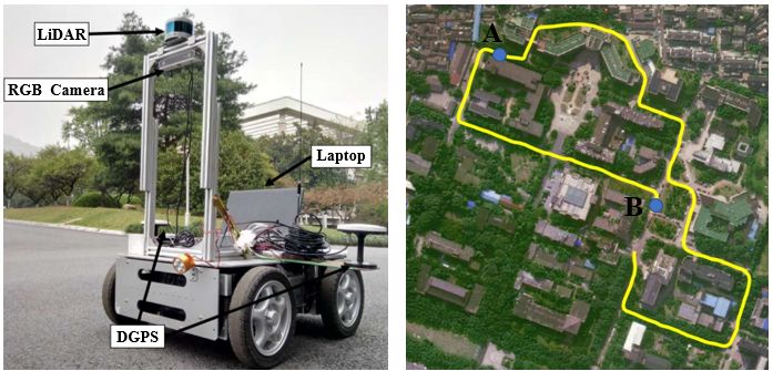
TABLE I: Comparison results with the average recall@1 and
recall@1% of different networks on the Oxford dataset.

                        Ave recall@1    Ave recall@1%
         PN-VLAD           67.94            81.01
          LPD-Net          86.28            94.42
        Img-VLAD           64.47            85.24
          Aug-Net          79.47            91.24
      Vis-VLAD(ours)       57.62            83.05
      Ele-VLAD(ours)       82.49            93.61
      Sum-First(ours)      82.44            92.71
      Con-First(ours)      84.82            93.62
                                                                  Fig. 4: Average recall@N(%) of different networks on the
      Sum-Four(ours)       86.23            94.43                 Oxford dataset.
      Con-Four(ours)       88.93            96.13

TABLE II: Average timing for computing a single instance
using NVIDIA 2080 Ti.

        Network          Avg. computational cost per descriptor
       PN-VLAD                         8.44ms
        LPD-Net                        15.28ms
     Img-NetVLAD                       62.28ms
        Aug-Net                        18.80ms
   CORAL-VLAD(ours)                    11.19ms

                                                                  Fig. 5: Networks limitations. These are incorrect matches
A. Datasets and settings                                          retrieved by our network, where (a) is the query, (b) is the
                                                                  wrong match, and (c) shows the true match.
   We choose the Oxford Robotcar dataset [15] for training
and testing. The car equipped with LiDAR sensors and
                                                                  B. Place recognition results on the Oxford dataset
cameras repeatedly drives through the same regions in one
year and collects data in large-scale and long-term conditions       We present qualitative results to demonstrate the feasibility
across weather, season and illumination. To create training       of our CORAL-VLAD on the Oxford dataset under chang-
tuples, we define the similar observations with a relative        ing scene conditions. The common assessment indicators
distance less than 10m and heading difference less than 30        of place recognition - average recall@1 and the average
degrees as positive pairs, and those at least 50m apart as        recall@1% are used to evaluate the network performance.
negative pairs. Referring to the data splitting rules of [1],     For fairness, the final global descriptor dimensions of all
we obtain 21636 training tuples from 44 sequences of the          networks are set to 256.
original dataset and 3011 testing samples from 23 sequences.         Ablation study on fusion strategy We test our compound
To keep large overlapping regions between the camera image        network with four feature fusion strategies operating on the
and the elevation image, the elevation map is set with the size   intermediate visual feature map and the structural feature
of 80×80 and the resolution of 0.5m. The input of the visual      map, including (a) element-wise summarization in the first
image is downscaled into 112 × 112 for extracting visual          residual block (Sum-First), (b) element-wise concatenation
features efficiently. Furthermore, as scans are accumulated by    in the first residual block (Con-First), (c) element-wise sum-
2D LiDAR scans at fixed intervals, there are some incomplete      marization in four residual blocks (Sum-Four), (d) element-
samples on the dataset. We discard them when generating the       wise concatenation in four residual blocks (Con-Four). The
elevation image.                                                  results are shown in Fig. 4 and Tab. I, the multi-scale fusion
   Generalization settings We choose KITTI dataset [7]            strategies outperform the single-scale due to the adequate
to evaluate the generalization performance across city and        information. And the better performance of concatenation
sensor configurations. Only Sequence 00 which visits the          than summation contributes to the intact information. In the
same places repeatedly is used. The first 170s of Sequence 00     following experiments, we use our network with the Con-
are used to construct the reference map and the rest are used     Four fusion strategy as the final version, denoted as CORAL-
as localization queries. The second dataset for generalization    VLAD.
evaluation is collected by ourselves in different seasons,           Ablation study on sensor modal Furthermore, to inves-
namely YQ. Data in overcast scene and snowy scene are used        tigate the contribution of the fusion step, we separate our
for mapping and query respectively. For a fair comparison,        fusion architecture into an independent visual stream and
the same criteria on Oxford Robotcar dataset are applied.         structural stream with a shared NetVLAD module to generate
                                                                  the global descriptor, called Vision NetVLAD(Vis-VLAD)
                                                                  and Elevation image NetVLAD(Ele-VLAD). The results are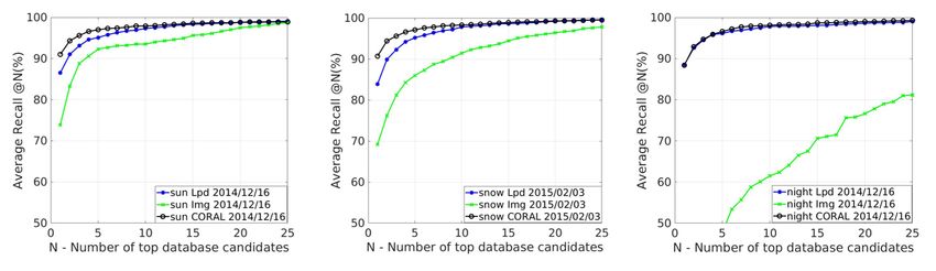
Fig. 6: Average recall@N(%) with LPD-Net(Lpd), Img-VLAD(Img) and CORAL-VLAD(CORAL) under different scene
conditions on the Oxford dataset.

also shown in Fig. 4 and Tab. I. Except for the fusion strategy   TABLE III: Comparison generalization results of the average
of Sum-First, results have been significantly improved using      recall@1(%) on the KITTI and YQ dataset
composite features. Furthermore, the results for single modal
place recognition are shown, validating the correct design                Network         KITTI laser   KITTI stereo    YQ
                                                                         PN-VLAD            72.43          65.43       40.36
and implementation of our method.
                                                                          LPD-Net           74.58          65.82       62.35
    Comparison with the-state-of-art methods We compare
                                                                          Aug-Net           75.60          70.56       66.91
our method with the state-of-the-art single modal place               CORAL-VLAD(ours)      76.43          70.77       73.82
recognition methods, PointNetVLAD (PN-VLAD) [1], LPD-
Net [13] and Img-VLAD [2], as well as bi-modal place
recognition method, compound network (Aug-Net)[19].               obtains lots of incorrect matches. Accordingly, CORAL-
    Using only structural data input, the performance of our      VLAD has minimal improvement over LPD-Net in such
Ele-VLAD is better than PN-VLAD, yet slightly worse               condition, showing the limitation of additional visual modal.
than LPD-Net. Inputs of LPD-Net and PN-VLAD are 4096                 Cases study Fig. 1 shows some of the successfully
filtered points with detailed 3D structural information of the    matched results in changing environments. We can observe
environment while the elevation image only has 40 × 40            that our network has learned robust features and alleviated
grids with one-channel elevation. It also proves effectiveness    the negative effect brought by dynamic obstacles and vari-
of the elevation image for representing 3D geometric data.        ations in illumination. Fig. 5 shows three wrong cases. We
Although providing a rich appearance context, Vis-VLAD            can see that the network is confused in the same scenes with
and Img-VLAD cannot outperform Ele-VLAD, which proves             opposite viewpoints (top row) and a few overlapping areas
that the elevation image representation is more robust under      (middle row and bottom row).
environment variations. Results are shown in Fig. 1. Mean-           Comparison on efficiency We further evaluate the run-
while, there are many over-exposed images on the Oxford           ning time of the network. Due to the use of lightweight
dataset, causing loss of visual features.                         network backbones and compact structural representation,
    Using composite descriptors, the performance of CORAL-        our network implementation takes about 11ms which is
VLAD exceeds all other methods, including Aug-Net. Note           faster than all methods except PN-VLAD shown in Tab.
that there is a difference in the Aug-Net from [19], since we     II. For generating the elevation map, we have a GPU-based
employ the PN-VLAD splitting rules clarified in [1] to ensure     implementation at almost 30Hz as shown in [21], achieving
consistency among all methods. All comparison network             real-time performance for robotics applications.
training sessions last no longer than 24h. We suppose that
the main reason for the slightly worse results of Aug-Net is
the incompleteness of the 3D volume based representation.         C. Generalization evaluation
    Comparison under different conditions We compare                 To analyze the generalization of our network, we evaluate
the performance of LPD-Net, Img-VLAD, CORAL-VLAD,                 our network on the YQ and KITTI datasets using the
which use inputs in different representation modalities under     model trained on the Oxford Robotcar dataset. These cross-
changing scene conditions. Fig. 6 shows the results when          city datasets consist of unobserved conditions with different
queries are taken from three different scene conditions           sensor configurations, including sensor types and extrinsic
against the testing database on the Oxford database (except       parameters. Specifically, KITTI laser uses the point cloud
query run). It can be seen that the huge variants of environ-     collected by LiDAR while KITTI stereo uses the point cloud
mental conditions have little impact on retrieval performance     generated from stereo images.
using structural cues. As almost all corresponding visual            In the case of KITTI laser dataset, the elevation image
features are lost at night scene, the visual-based approach       is generated in real-time using Velodyne 64 HDL LiDAR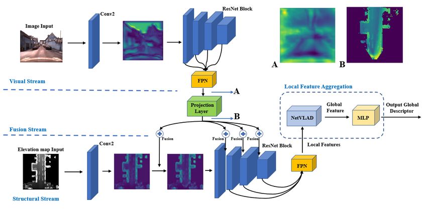
Fig. 7: Matching examples on the KITTI dataset. The left
column shows the correct match on the KITTI stereo and the
right column shows the correct match on the KITTI laser.
                                                                 Fig. 9: Matching examples on the YQ dataset. The left
                                                                 column shows the correct matching example at point A in
                                                                 Fig. 8. The right column shows the matching result at point
                                                                 B in Fig. 8.

                                                                 features in the same consistent BEV frame, which can han-
                                                                 dle various environmental variances like viewpoint changes,
                                                                 illuminations, and structure losses. We show that the method
                                                                 performs best on the Oxford Robotcar dataset, as well as
                                                                 generalization test on conditions and sensor configurations
                                                                 using the cross-city datasets of the KITTI dataset and YQ
Fig. 8: The collection of the YQ dataset. The left image         dataset.
shows the data collection platform. The yellow line of the
right image shows the trajectory of the data collection on our                   VI. ACKNOWLEDGMENT
campus.                                                            This work was supported in part by the National Nature
                                                                 Science Foundation of China under Grant 61903332, and in
shown in Fig. 7 and our network outperforms other methods        part by the Natural Science Foundation of Zhejiang Province
in Tab. III. Although there is noise involved during the         under grant number LGG21F030012.
calculation of the disparity map on the KITTI stereo dataset,                           R EFERENCES
generated elevation maps become blurred, which loses some
                                                                  [1] Mikaela Angelina Uy and Gim Hee Lee. “Point-
structural information and introduces inaccurate matches
                                                                      netvlad: Deep point cloud based retrieval for large-
between pixels and 3D points. CORAL-VLAD still achieves
                                                                      scale place recognition”. In: Proceedings of the IEEE
the best results, demonstrating the validity of our network
                                                                      Conference on Computer Vision and Pattern Recogni-
for pure vision-based applications.
                                                                      tion. 2018, pp. 4470–4479.
   Additionally, we conduct experiments under different
                                                                  [2] Relja Arandjelovic et al. “NetVLAD: CNN archi-
weather conditions on our campus. Unlike evaluating with
                                                                      tecture for weakly supervised place recognition”. In:
similar conditions at a short period of time on the KITTI
                                                                      Proceedings of the IEEE conference on computer
dataset, the unmanned ground vehicle equipped with a Li-
                                                                      vision and pattern recognition. 2016, pp. 5297–5307.
DAR and an RGB camera collects sensor data on sunny
                                                                  [3] Herbert Bay et al. “Speeded-up robust features
days in spring and snowy days in winter denoted as YQ
                                                                      (SURF)”. In: Computer vision and image understand-
dataset. The data collection platform is shown in Fig. 8. In
                                                                      ing 110.3 (2008), pp. 346–359.
addition, DGPS provides the ground-truth position to check
                                                                  [4] Weihua Chen et al. “Beyond triplet loss: a deep
the correctness of the matching results. The summer-overcast
                                                                      quadruplet network for person re-identification”. In:
scene of the YQ dataset is utilized as the reference database,
                                                                      Proceedings of the IEEE Conference on Computer
and the winter-snow scene as the query dataset. Matching
                                                                      Vision and Pattern Recognition. 2017, pp. 403–412.
examples are shown in Fig. 9, formulating a generalization
                                                                  [5] Péter Fankhauser et al. “Kinect v2 for mobile robot
evaluation on both conditions and sensor configurations.
                                                                      navigation: Evaluation and modeling”. In: 2015 Inter-
CORAL-VLAD still achieves the best performance in this
                                                                      national Conference on Advanced Robotics (ICAR).
scenario as shown in Tab. III, because of the elevation image
                                                                      IEEE. 2015, pp. 388–394.
based structural representation, transforming the texture into
                                                                  [6] Dorian Gálvez-López and Juan D Tardos. “Bags of
a geometric sensible representation.
                                                                      binary words for fast place recognition in image
                                                                      sequences”. In: IEEE Transactions on Robotics 28.5
                     V. C ONCLUSION
                                                                      (2012), pp. 1188–1197.
   In this paper, we introduce the elevation map as the
structural information and propose the bi-modal environment
representation CORAL to fuse the structural and visual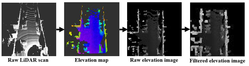
[7]   Andreas Geiger, Philip Lenz, and Raquel Urtasun.
                                                                         Conference on Robotics and Biomimetics (ROBIO).
       “Are we ready for autonomous driving? the kitti
                                                                         IEEE. 2019, pp. 734–740.
       vision benchmark suite”. In: 2012 IEEE Conference
                                                                  [22]   Charles R Qi et al. “Pointnet: Deep learning on point
       on Computer Vision and Pattern Recognition. IEEE.
                                                                         sets for 3d classification and segmentation”. In: Pro-
       2012, pp. 3354–3361.
                                                                         ceedings of the IEEE conference on computer vision
 [8]   Kaiming He et al. “Deep residual learning for image
                                                                         and pattern recognition. 2017, pp. 652–660.
       recognition”. In: Proceedings of the IEEE conference
                                                                  [23]   Charles R Qi et al. “Volumetric and multi-view cnns
       on computer vision and pattern recognition. 2016,
                                                                         for object classification on 3d data”. In: Proceedings of
       pp. 770–778.
                                                                         the IEEE conference on computer vision and pattern
 [9]   Herve Jegou et al. “Aggregating local image descrip-
                                                                         recognition. 2016, pp. 5648–5656.
       tors into compact codes”. In: IEEE transactions on
                                                                  [24]   Filip Radenović, Giorgos Tolias, and Ondřej Chum.
       pattern analysis and machine intelligence 34.9 (2011),
                                                                         “Fine-tuning CNN image retrieval with no human
       pp. 1704–1716.
                                                                         annotation”. In: IEEE transactions on pattern analysis
[10]   Hervé Jégou et al. “Aggregating local descriptors
                                                                         and machine intelligence 41.7 (2018), pp. 1655–1668.
       into a compact image representation”. In: 2010 IEEE
                                                                  [25]   Radu Bogdan Rusu et al. “Aligning point cloud
       computer society conference on computer vision and
                                                                         views using persistent feature histograms”. In: 2008
       pattern recognition. IEEE. 2010, pp. 3304–3311.
                                                                         IEEE/RSJ international conference on intelligent
[11]   G. Kim, B. Park, and A. Kim. “1-Day Learning, 1-
                                                                         robots and systems. IEEE. 2008, pp. 3384–3391.
       Year Localization: Long-Term LiDAR Localization
                                                                  [26]   Samuele Salti, Federico Tombari, and Luigi Di Ste-
       Using Scan Context Image”. In: IEEE Robotics and
                                                                         fano. “SHOT: Unique signatures of histograms for
       Automation Letters 4.2 (Apr. 2019), pp. 1948–1955.
                                                                         surface and texture description”. In: Computer Vision
[12]   Ming Liang et al. “Deep continuous fusion for multi-
                                                                         and Image Understanding 125 (2014), pp. 251–264.
       sensor 3d object detection”. In: Proceedings of the
                                                                  [27]   Karen Simonyan and Andrew Zisserman. “Very deep
       European Conference on Computer Vision (ECCV).
                                                                         convolutional networks for large-scale image recogni-
       2018, pp. 641–656.
                                                                         tion”. In: arXiv preprint arXiv:1409.1556 (2014).
[13]   Zhe Liu et al. “Lpd-net: 3d point cloud learning for
                                                                  [28]   Li Tang et al. “Adversarial feature disentanglement
       large-scale place recognition and environment analy-
                                                                         for place recognition across changing appearance”. In:
       sis”. In: Proceedings of the IEEE International Con-
                                                                         2020 IEEE International Conference on Robotics and
       ference on Computer Vision. 2019, pp. 2831–2840.
                                                                         Automation (ICRA). IEEE. 2020, pp. 1301–1307.
[14]   David G Lowe. “Distinctive image features from
                                                                  [29]   Zining Wang, Wei Zhan, and Masayoshi Tomizuka.
       scale-invariant keypoints”. In: International journal of
                                                                         “Fusing bird’s eye view lidar point cloud and front
       computer vision 60.2 (2004), pp. 91–110.
                                                                         view camera image for 3d object detection”. In:
[15]   Will Maddern et al. “1 year, 1000 km: The Oxford
                                                                         2018 IEEE Intelligent Vehicles Symposium (IV). IEEE.
       RobotCar dataset”. In: The International Journal of
                                                                         2018, pp. 1–6.
       Robotics Research 36.1 (2017), pp. 3–15.
                                                                  [30]   Shaorong Xie et al. “Large-Scale Place Recognition
[16]   Raul Mur-Artal, Jose Maria Martinez Montiel, and
                                                                         Based on Camera-LiDAR Fused Descriptor”. In: Sen-
       Juan D Tardos. “ORB-SLAM: a versatile and accurate
                                                                         sors 20.10 (2020), p. 2870.
       monocular SLAM system”. In: IEEE transactions on
                                                                  [31]   Xuecheng Xu et al. “DiSCO: Differentiable Scan
       robotics 31.5 (2015), pp. 1147–1163.
                                                                         Context with Orientation”. In: arXiv preprint
[17]   Raul Mur-Artal and Juan D Tardós. “Orb-slam2: An
                                                                         arXiv:2010.10949 (2020).
       open-source slam system for monocular, stereo, and
                                                                  [32]   Huan Yin et al. “LocNet: Global localization in 3D
       rgb-d cameras”. In: IEEE Transactions on Robotics
                                                                         point clouds for mobile vehicles”. In: 2018 IEEE Intel-
       33.5 (2017), pp. 1255–1262.
                                                                         ligent Vehicles Symposium (IV). IEEE. 2018, pp. 728–
[18]   Hyeonwoo Noh et al. “Large-scale image retrieval
                                                                         733.
       with attentive deep local features”. In: Proceedings of
                                                                  [33]   Wenxiao Zhang and Chunxia Xiao. “PCAN: 3D at-
       the IEEE international conference on computer vision.
                                                                         tention map learning using contextual information for
       2017, pp. 3456–3465.
                                                                         point cloud based retrieval”. In: Proceedings of the
[19]   Amadeus Oertel, Titus Cieslewski, and Davide Scara-
                                                                         IEEE Conference on Computer Vision and Pattern
       muzza. “Augmenting Visual Place Recognition with
                                                                         Recognition. 2019, pp. 12436–12445.
       Structural Cues”. In: arXiv preprint arXiv:2003.00278
                                                                  [34]   Yin Zhou and Oncel Tuzel. “Voxelnet: End-to-end
       (2020).
                                                                         learning for point cloud based 3d object detection”.
[20]   Yiyuan Pan et al. “GEM: online globally consistent
                                                                         In: Proceedings of the IEEE Conference on Computer
       dense elevation mapping for unstructured terrain”. In:
                                                                         Vision and Pattern Recognition. 2018, pp. 4490–4499.
       IEEE Transactions on Instrumentation and Measure-
       ment (2020).
[21]   Yiyuan Pan et al. “GPU accelerated real-time
       traversability mapping”. In: 2019 IEEE International
You can also read