Comparing interpretation methods in mental state decoding analyses with deep learning models - arXiv
←
→
Page content transcription
If your browser does not render page correctly, please read the page content below
Comparing interpretation methods in mental state decoding
                                                        analyses with deep learning models
                                                            Armin W. Thomas∩,∨,◦ , Christopher Rét , and Russell A. Poldrack∩,∨,◦
                                                                  ∩
arXiv:2205.15581v2 [q-bio.NC] 14 Oct 2022

                                                                   Stanford Data Science, Stanford University, Stanford, CA, USA
                                                                   ∨ Dept. of Psychology, Stanford University, Stanford, CA, USA
                                                               t Dept. of Computer Science, Stanford University, Stanford, CA, USA
                                                                                  ◦ {athms,russpold}@stanford.edu

                                                                                           July 2022

                                                                                            Abstract
                                                     Deep learning (DL) models find increasing application in mental state decoding, where
                                                 researchers seek to understand the mapping between mental states (e.g., perceiving fear or
                                                 joy) and brain activity by identifying those brain regions (and networks) whose activity al-
                                                 lows to accurately identify (i.e., decode) these states. Once a DL model has been trained to
                                                 accurately decode a set of mental states, neuroimaging researchers often make use of inter-
                                                 pretation methods from explainable artificial intelligence research to understand the model’s
                                                 learned mappings between mental states and brain activity. Here, we compare the explana-
                                                 tion performance of prominent interpretation methods in a mental state decoding analysis of
                                                 three functional Magnetic Resonance Imaging (fMRI) datasets. Our findings demonstrate a
                                                 gradient between two key characteristics of an explanation in mental state decoding, namely,
                                                 its biological plausibility and faithfulness: interpretation methods with high explanation faith-
                                                 fulness, which capture the model’s decision process well, generally provide explanations that
                                                 are biologically less plausible than the explanations of interpretation methods with less ex-
                                                 planation faithfulness. Based on this finding, we provide specific recommendations for the
                                                 application of interpretation methods in mental state decoding.

                                                Deep learning (DL) models have celebrated immense successes in many areas of research and
                                            industry (Goodfellow et al., 2016, LeCun et al., 2015). This success is often attributed to their un-
                                            matched ability to learn versatile representations of complex datasets, allowing them to associate
                                            a target signal with varying patterns in minimally-preprocessed (or raw) data. Due to their empir-
                                            ical success, neuroimaging researchers have started applying DL models to mental state decoding
                                            analyses (e.g., Mensch et al., 2021, Plis et al., 2014, Thomas et al., 2019, VanRullen and Reddy,
                                            2019, Wang et al., 2020, Zhang et al., 2021). In these analyses, researchers seek to understand
                                            how specific mental states (e.g., answering questions about a prose story or math problem) are
                                            represented in the brain by identifying brain regions (or networks of brain regions) whose activity
                                            patterns allow accurate identification (i.e., decoding) of these mental states (Haynes and Rees,
                                            2006).
                                                Once a DL model has been trained to accurately decode a set of mental states from brain
                                            activity, researchers often make use of interpretation methods from explainable artificial intelli-
                                            gence research (XAI; Doshi-Velez and Kim, 2017, Samek et al., 2021) to gain insights into the
                                            models’ learned mappings between mental states and brain activity, seeking to overcome the un-
                                            interpretability of DL models (Rudin, 2019). From the wealth of existing interpretation meth-
                                            ods (Gilpin et al., 2018, Linardatos et al., 2021), neuroimaging researchers most often utilize
                                            attribution (i.e., heatmapping) methods, which attribute a relevance to each feature value of an

                                                                                                1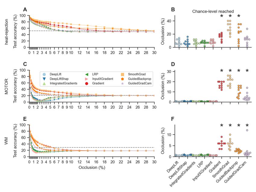
input for the resulting decoding decision of a DL model, resulting in a heatmap of relevance val-
ues (Samek et al., 2021). On a high level, prominent attribution methods in the mental state
decoding literature can be grouped into sensitivity analyses (e.g., Simonyan et al., 2014, Smilkov
et al., 2017, Springenberg et al., 2015), reference-based attributions (e.g., Lundberg and Lee, 2017,
Shrikumar et al., 2017, Sundararajan et al., 2017), and backward decompositions (e.g., Bach et al.,
2015, Montavon et al., 2017). Sensitivity analyses, such as Gradient Analysis (Simonyan et al.,
2014), attribute relevance to input features according to how sensitively a model’s decoding decision
responds to a feature’s value. Reference-based attributions, such as DeepLift (Shrikumar et al.,
2017) or Integrated Gradients (Sundararajan et al., 2017), by contrast, attribute relevance to input
features by comparing the model’s response to a given input to its response to a reference input
(e.g., a neutral input). Backward decompositions, such as Layer-wise relevance propagation (LRP;
Bach et al., 2015), on the other hand, attribute relevance to input features by decomposing the
decoding decision of a DL model in a backward pass through the model into the contributions of
lower-level model units to the decision, up to the input space, where a contribution for each input
feature can be defined.
    Given the wealth of existing attribution methods, neuroimaging researchers interested in in-
terpreting the mental state decoding decisions of DL models are faced with the task of choosing
a method for their particular analysis and research question. Yet, in many cases, the explana-
tions of different attribution methods are difficult to visually discern, making it challenging to
compare and evaluate their quality. Even further, it is unclear whether related empirical findings
from computer vision (CV; Adebayo et al., 2018, Kindermans et al., 2019, Samek et al., 2017)
and natural language processing (NLP; Ding and Koehn, 2021, Jacovi and Goldberg, 2020, Jain
and Wallace, 2019), on the relative performance of different attribution methods, generalize to
neuroimaging data. There, researchers have often argued that reference-based attributions and
backward decompositions are superior to sensitivity analyses because they capture the decision
process of DL models more faithfully. Yet, mental state decoding is distinct from most CV and
NLP applications in that researchers seek to understand the association of input data (i.e., brain
activity) and decoding targets (i.e., mental states), whereas CV and NLP are often solely concerned
with predictive performances (Lipton and Steinhardt, 2018). To date, it is therefore unclear how
prominent attribution methods compare in providing insights into the association of brain activity
and mental states learned by DL models.
    In this work, we compare the explanation performance of prominent attribution methods in
a mental state decoding analysis of three functional Magnetic Resonance (fMRI) datasets. To
compare performances, we use two main criteria: First, we evaluate the biological plausibility
of the explanations of an attribution method by testing whether they identify all voxels of the
input whose activity pattern is reliably associated with the decoded mental state. To this end,
we compare its explanations to the results of a standard general linear model (GLM; Holmes and
Friston, 1998) analysis of the fMRI data. We find that the explanations of sensitivity analyses
are generally more similar to the results of a GLM analysis when compared to the explanations
of reference-based attributions and backward decompositions. Second, to understand how well
the explanations capture the decision process of the DL model, we evaluate their faithfulness by
testing whether they correctly identify those voxels of the input whose activity is necessary for the
model to accurately decode the mental states. We find that the explanations of reference-based
attributions and backward decompositions are generally more faithful than those of sensitivity
analyses.
    Taken together, these findings lead us to a twofold recommendation for attribution meth-
ods in mental state decoding: If researchers want to understand the decision process of a DL
model in mental state decoding, we recommend reference-based attribution methods (such as
DeepLift (Shrikumar et al., 2017), DeepLift SHAP Lundberg and Lee (2017), and Integrated Gra-
dients (Sundararajan et al., 2017)), and backward decompositions (such as LRP (Bach et al., 2015))
because their explanations are the most faithful in our analyses. By contrast, if researchers want to

                                                 2
understand the association between mental states and brain activity, and merely use DL models as
a tool to study this association, we recommend sensitivity analyses (such as Gradient Analysis (Si-
monyan et al., 2014), SmoothGrad (Smilkov et al., 2017), Guided Backpropagation (Springenberg
et al., 2015), and Guided GradCam (Selvaraju et al., 2017)) because their explanations align better
with the results of standard analysis approaches for fMRI data.

1       Methods
1.1     Data
We analyzed three fMRI datasets in this study, namely, fMRI data of 44 randomly-selected indi-
viduals in the motor task of the Human Connectome Project (HCP; Van Essen et al., 2013), 44
randomly-selected individuals in the HCP’s working memory (WM) task, and 58 individuals in
a pain and social rejection experiment published by Woo et al. (2014). We refer to these three
datasets respectively as ”MOTOR”, ”WM”, and ”heat-rejection” in the following and provide a
brief overview of their experiment tasks as well as details on the fMRI acquisition and preprocessing.
For any further methodological details, we refer the reader to the original publications (Van Essen
et al., 2013, Woo et al., 2014).

1.1.1    Experiment tasks
Heat-rejection: The heat-rejection dataset comprises fMRI data from two experimental tasks.
In the rejection task, individuals either see head shots of an ex-partner with a cue-phrase beneath
the photo directing them to think about how they felt during the break-up (rejection) or a head
shot of a close friend with a cue-phrase directing them to think about a specific positive experience
with this friend (no rejection). In the somatic pain task, individuals focus on a hot (painful) or
warm (not painful) stimulus that is delivered to their left forearm (with temperatures calibrated
to each participant). Each rejection trial begins with a 7 s fixation cross, followed by a 15 s
presentation period of a photo (ex-partner or friend), a 5 s five-point affect rating period, and 18
s of a visuo-spatial control task in which individuals see an arrow pointing left or right and are
asked to indicate in which direction the arrow is pointing. Heat trials are identical in structure
to rejection trials with the exception that individuals see a fixation cross during the 15 s thermal
stimulation period (consisting of a 1.5 s temperature ramp up/down and 12 s at peak temperature)
and subsequently use the five-point rating scale to report their experienced pain level.

MOTOR: In the HCP’s motor task, individuals see visual cues asking them to tap their left or
right fingers, squeeze their left or right toes or move their tongue. The task was presented in blocks
of 12 s, each including one movement type, preceded by 3 s cue. Two fMRI runs were collected for
this task, each comprising two blocks of tongue movements, four blocks of hand movements (two
left, two right), and four blocks of foot movements (again, two left and two right) as well as three
15 s fixation blocks.

WM: In the HCP’s WM task, individuals see images of one of four different stimulus types
(namely, body parts, faces, places or tools). In one half of the task blocks, individuals are asked
to indicate whether the current stimulus is the same as the stimulus that was shown 2 before (2-
back). In the other half of the task blocks, individuals are asked to indicate whether the currently
presented stimulus is the same as a target stimulus that was shown at the beginning of the block
(0-back). Two fMRI runs were collected for this task, each comprising eight task (25 s each) and
four fixation blocks (15 s each). Each task block consists of 10 trials (2.5 s each) of 2 s stimulus
presentation and 0.5 s interstimulus interval. Note that we pool the data of the two N-back

                                                  3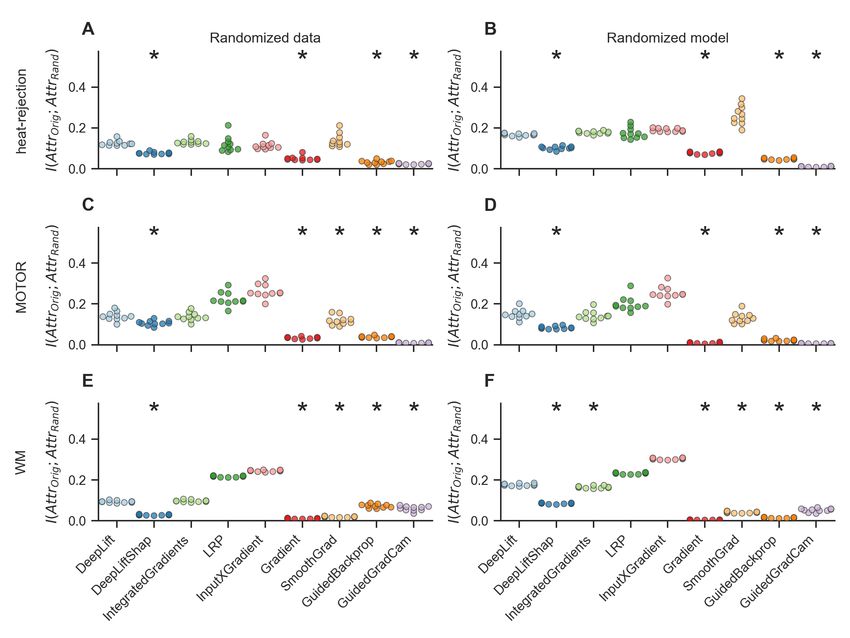
conditions because we are not interested in identifying any effect of the N-back condition on brain
activity.

1.1.2   FMRI data acquisition
Heat-rejection:       Whole-brain EPI acquisitions were acquired on a GE 1.5 T scanner using a
T2*-weighted spiral in-out sequence developed by Dr Gary Glover with TR = 2,000 ms, TE =
40 ms, flip angle = 84, FOV = 22 cm, and 24 axial slices with 3.5 × 3.5 × 4.5 mm voxels parallel
to the anterior commissure-posterior commissure line (for further methodological details on fMRI
data acquisition, see Woo et al., 2014)).

Human Connectome Project: Whole-brain EPI acquisitions were acquired with a 32-channel
head coil on a modified 3T Siemens Skyra with TR = 720 ms, TE = 33.1 ms, flip angle = 52,
in-plane FOV = 20, 8 × 18cm, and 72 slices with 2.0 mm isotropic voxels. Two fMRI runs were
acquired for each task, one with a right-to-left and the other with a left-to-right phase encoding (for
further methodological details on fMRI data acquisition, see Uğurbil et al., 2013).

1.1.3   FMRI data preprocessing
Human Connectome Project: We preprocessed the fMRI data of the MOTOR and WM
datasets with fmriprep 20.2.3 (Esteban et al., 2019). A detailed description of all preprocessing
steps can be found in Appendix A.1.1.

Heat-rejection: The data preprocessing was performed by the original authors (see Woo et al.,
2014) and included removal of the first four volumes of each fMRI run to allow for image intensity
stabilization, slice timing correction (realignment) with SPM8, spatial warping to SPM’s normative
atlas using warping parameters estimated from co-registered, high-resolution structural images,
interpolated to 2 × 2 × 2 mm voxels, and spatial smoothing with an 8 mm FWHM Gaussian
kernel.

1.2     Statistical parametric maps
1.2.1   Trial-level maps
We performed all of our analyses on trial-level voxel-wise statistical parametric maps (Friston
et al., 1994) that were computed for each experiment trial of a dataset. We refer to these maps as
trial-level blood-oxygen-level-dependent (BOLD) maps throughout the rest of the manuscript.

Heat-rejection: Trial-level BOLD maps were computed by the original authors (see Woo et al.,
2014) in an analysis that included boxcar regressors, convolved with the canonical haemodynamic
response function (HRF), for the 15 s photo or pain periods, the subsequent 5 s affect or pain rating
period, and the 18 s period of the visuospatial control task (leaving the fixation-cross periods as
unmodeled baselines), and a boxcar regressor for each individual trial. In addition, nuisance
covariates of no interest were included in the analysis representing a linear drift across time within
each run, the six estimated head movement parameters for each run (x, y, z, roll, pitch and yaw;
mean-centered) as well as their squares, derivatives, and squared derivatives, and indicator vectors
for outlier time points (for details on outlier detection, see Woo et al., 2014).

Human Connectome Project:           We computed trial-level BOLD maps by the use of Nilearn
0.9.0 (Abraham et al., 2014a). This analysis included boxcar regressors for each trial type (i.e.,

                                                  4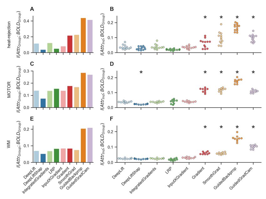
body, face, place, tool for the WM task and left/right foot, left/right finger, and tongue for the MO-
TOR task), which we convolved with a standard Glover HRF (as implemented by Nilearn (Abra-
ham et al., 2014a); leaving the fixation periods as unmodelled baselines), and a boxcar regressor
for each individual trial. In addition, the analysis included nuissance regressors of no interest rep-
resenting the six estimated head movement parameters (x, y, z, roll, pitch and yaw) as well as their
squares, derivatives, and squared derivatives, the average signal of white matter and cerebrospinal
fluid masks, the global signal, and a set of low-frequency regressors to account for slow signal drifts
below 128 s.

1.2.2   Subject- and group-level maps
To aggregate the trial-level BOLD maps to the subject- and group-level, we used a standard
two-stage analysis procedure as proposed by (Holmes and Friston, 1998).
    The subject-level analysis included a binary indicator variable for each mental state of a dataset,
which we used to contrast each mental state of a dataset against all other mental states of the
dataset. Note that the subject-level analysis of the two HCP datasets (WM and MOTOR) also
included a binary nuissance variable for each of the two fMRI runs.
    The group-level analysis included a binary indicator variable for each subject-level contrast type
(i.e., mental state) as well as a binary nuisance variable for each included individual. Accordingly,
the resulting group-level contrast maps correspond to a paired, two-sample t-test over the subject-
level contrast maps. Note that we smoothed all subject-level contrast maps with a 5 mm FWHM
Gaussian kernel in the group-level analysis.

1.3     Training and test data
To create distinct training and test datasets, we separated the trial-level BOLD maps of each
dataset by assigning the maps of every 5th individual of a dataset to a test dataset and designating
the maps of all remaining individuals as training data.

1.4     Deep learning model
We use 3D-convolutional neural network architectures (3D-CNNs; LeCun et al., 1998) as mental
state decoding models, which are composed of a stack of 3D-convolution layers and a dense output
layer.
    A 3D-convolution layer consists of a set of 3D-kernels that each learn specific features of an
input volume x. Each kernel k learns a volumetric feature that is convolved over the input, resulting
in an activation map Ak P that P
                               indicates
                                   P kthe presence of the learned feature   for each spatial location
of the input: Aki,j,l = g( m n z wm,n,z        xi+m−1,j+n−1,l+z−1 + bk ). Here, bk and wk represent
the bias and weights of the kernel, while g represents the rectified linear unit activation function
(g(x) = max(0, x)). The indices m, n, and z indicate the row, column, and height of the 3D-
convolution kernel, while i, j, and l indicate the coronal (i.e., row), saggital (i.e., column), and
axial (i.e., height) dimension of the activation map Ak . Note that the models move all convolution
kernels over their input at a stride size of 2, thus applying the kernels to every other value of a
layer’s input. The models further apply batch-normalization Ioffe and Szegedy (2015) to the linear
outputs of each convolution layer (before the non-linear activation).
    To make a decoding decision, the models flatten the activation maps A resulting from the last
convolution layer and pass the flattened maps to a dense softmax output   P layer, which predicts
a probability pc that input x represents mental state c: pc = σ(bc + i ai wic ), where b and w
                                                                                              xj
represent the layer’s bias and weights, while σ indicates the softmax function: σ(x)j = Pe exi .
                                                                                              i

                                                  5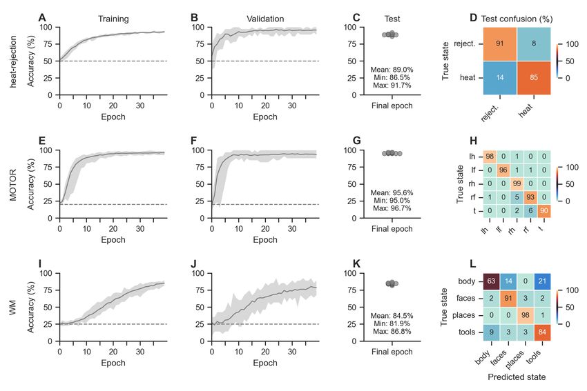
Figure 1: Attribution approaches. All considered attribution approaches η(·) seek to explain a mental
state decoding decision f (x) of model f (·) by attributing a relevance r to each feature of the input x for
the decision. Backward decompositions attribute relevance to input features by decomposing the decoding
decision in a backward pass through the model into the contributions of lower-level model units to the
decision, up to the input space, where a contribution for each input feature can be defined. Reference-
based attributions, by contrast, attribute relevance to input features by comparing the model’s response
to a given input to its response to a reference input x0 , often chosen to be neutral. Sensitivity analyses,
on the other hand, attribute relevance to input features according to how sensitively a model’s decoding
decision responds to an input feature’s value.

1.4.1   Training details
If not reported otherwise, we train models with stochastic gradient descent and the ADAM op-
timizer (Kingma and Ba, 2017) for 40 training epochs, where one epoch is defined as an entire
iteration over a dataset’s training data.

1.4.2   Hyper-parameter evaluation
For each dataset, we perform a grid search to determine a set of best-performing model and
optimization hyper-parameters. Specifically, we search over the number of model convolutional
layers (3, 4, and 5), the number of kernels per layer (4, 8, and 16), and the kernels’ size (3 and 5)
as well as the mini-batch size (32 and 64), learning rate (1e−4 and 1e−3 ), and dropout rate (25%
and 50%; applied to convolution layers) used during training (for an overview of the grid search
results, see section 2.1).

                                                     6
1.5 Attribution methods
We assume that the analyzed model represents some function f (·) mapping an input x ∈ RN to
some output f (x) ∈ R, such that: f (·) : RN → − R. In the following, we present a set of attribution
methods η(·) that seek to provide insights into this mapping by attributing a relevance score rn to
− RN .
each input feature n = 1, ..., N , quantifying its contribution to f (x), such that: η(·) : R →
On a high level, the presented attribution methods can be divided into sensitivity analyses,
reference-based attribution methods, and backward decompositions (see Fig. 1). Sensitivity anal-
yses quantify r by determining how sensitively f (x) responds to x. Reference-based attributions,
by contrast, determine r by contrasting the model’s response to a given input x to its response
to a reference input b. Backward decompositions, on the other hand, quantify r by sequentially
decomposing the model’s output f (x) in a backward pass through the model into the contributions
of the lower-layer model units to the predictions, until the input space is reached and a contribution
for each input feature can be defined.
Gradient Analysis (Simonyan et al., 2014, Zurada et al., 1994): represents the most
commonly used type of sensitivity analysis and defines rn as the partial derivative of f (x) with
respect to the input xn , such that: rn = | ∂f (x)
∂xn |. Relevance is thus assigned to those feature values
to which f (x) responds most sensitively.
SmoothGrad (Smilkov et al., 2017): represents an extension of Gradient Analysis to account
for sharp fluctuations of the gradient ∇f (x) = ∂f∂x
(x)
at small scales, which can otherwise lead to
noise in the resulting attributions. SmoothGrad therefore first randomly draws K samples (we set
K = 50) from the neighborhood of x by adding random Gaussian noise N (0, σ 2 ) with standard
deviation σ (we set σ = 1) to x, and subsequently averages the resulting absolute partial derivatives
1
PK 2
for each random sample to obtain relevances r: r = K 1 |∇f (x + N (0, σ ))|.
InputXGradient (Shrikumar et al., 2017): represents another extension of Gradient Anal-
ysis, which multiplies the gradient ∇f (x) by x, such that: r = ∇f (x) × x (where × indicates the
element-wise product). The intuition behind this approach comes from linear models, where the
product of input and model coefficient (here represented by the gradient) corresponds to the total
contribution of the associated feature to the model’s output.
Guided Backpropagation (Springenberg et al., 2015): represents an adaptation of Gradi-
ent Analysis tailored to CNN models that primarily use ReLU Agarap (2019) activation functions.
It overrides gradients of ReLU activation functions in the computation of the gradient ∇f (x) such
that only non-negative gradients are backpropagated.
Guided Gradient-weighted Class Activation Mapping (Guided GradCam) (Selvaraju
et al., 2017): represents another type of sensitivity analysis tailored to CNNs that combines
Guided Backpropagation with the GradCam (Selvaraju et al., 2017) technique. Specifically, Grad-
Cam first computes the gradient ∇f (x) with respect to the feature maps Ak ∈ RD of the last con-
volutional layer L closest to the model’s output ( ∂f (x)
∂Ak
) and then global-average pools the resulting
1
PD ∂f (x)
gradients to obtain an importance weight αk for each kernel k ∈ L: αk = D d=1 ∂Ak . Conceptu-
d
ally, ak captures the importance of feature map Ak for the decoded mental state. Next, GradCam
k
uses the importance weights
P αk kto combine the activation maps A to an aggregate heatmap of
relevances rA : rA = σ( k αk A ), where σ represents the ReLU function (σ(x) = max(0, x)).
Last, to obtain relevances r, Guided GradCam upsamples the relevances rA to the original input
dimension and multiplies the upsampled maps with the relevance attributions of an application of
Guided Backpropagation to f (x) (see above).
7Integrated Gradients (Sundararajan et al., 2017): represents a reference-based attribution
method that assigns relevance r by integrating the gradient ∇f (x) along a linear trajectory in
the input space, connecting the current input x to some neutral reference input b: rb = (x −
R1
b) α=0 δf (b+α(x−b))
δx . Integrated Gradients thus assigns relevance to input features according to
how much the model’s output changes when these features are scaled from the reference value
to their current value. In our analyses, we chose two reference inputs, namely, an all-zero input
b0 (as recommended in Sundararajan et al., 2017) as well as an average over all inputs in the
analyzed dataset bµ , and averaged over the two resulting attributions to obtain relevance values r:
r = 0.5r0 + 0.5rµ .
Deep Learning Important FeaTures (DeepLift) DeepLift (Shrikumar et al., 2017):
represents another type of reference-based attribution method. Similar to Integrated Gradients,
DeepLift determines relevances r by comparing model responses for a given input x to the model’s
response to some neutral reference input b. To this end, DeepLift defines a contribution score
C∆xn ∆f (x) , describing the difference-from-reference response ∆f (x) = f (x)−f (b) that is attributed
PN
to a difference-from-reference in the input ∆x = x − b. Note that n=1 C∆xn ∆f (x) = ∆f (x).
To compute these contribution scores, DeepLift uses multipliers m∆xn ∆f (x) that are defined as
C
m∆x∆f (x) = ∆x∆f ∆x
(x)
and thereby quantify the contribution of ∆x to ∆f (x), scaled by ∆x. For
any unit x(l) in model layer l and any unit x(l−1) in the preceding layer l−1, these multipliers can be
P (l)
computed as: m∆x(l−1) ∆f (x) = j m∆x(l−1) ∆x(l) m∆x(l) ∆f (x) (where ∆xj indicates the difference
n n j j
in input feature j of layer l to its value for the reference input), in line with the chain rule. Relevance
rn for input feature n can then be obtained as: rn = C∆xn ∆f (x) = ∆xn m∆xn ∆f (x) . In its basic
formulation, DeepLift uses two rules to compute contribution scores: The linear rule applies to
dense and convolution layers, which compute a = w0 + n wn xn (where w0 and w indicate bias
P
C n ∆a
and weights and x the input), and defines C∆xn ∆a = ∆xn wn and accordingly m∆xn ∆a = ∆x ∆xn .
The rescale rule applies to all non-linear transformations σ(a) (e.g., ReLU or sigmoid functions)
C
and defines C∆x∆σ(a) = ∆σ(a) and accordingly m∆x∆σ(a) = ∆x∆σ(a) ∆x .
DeepLift SHapley Additive exPlanation (DeepLift SHAP) (Lundberg and Lee, 2017):
combines DeepLift with SHAP, a method for computing Shapley values (Shapley, 1952) for a
conditional expectation function of the analyzed model. Specifically, SHAP values attribute to
each input feature the change in expected model prediction conditioned on a feature of interest.
To approximate SHAP values using DeepLift for a given input x, DeepLift SHAP draws K (we
set K = 50) random samples from the data (to approximate the set of other possible feature
coalitions) and averages over the DeepLift attributions for each random sample, when treating the
random sample as a reference input b.
Layer-wise relevance propagation (LRP) (Bach et al., 2015): represents a backward
decomposition method. Let i and j be the indices of two models units in successive model layers
(l+1)
l and l + 1 and rj the relevance of unit j for f (x). To redistribute relevance between layers,
several rules have been proposed (Bach et al., 2015, Kohlbrenner et al., 2020, Montavon et al.,
(l) P aw (l+1)
2019), which generally follow from ri = j P iaiijwij rj (where a and w represent the input
i
and weight of model unit i in layer l). Importantly, LRP conserves relevance between layers, such
P P (l) P (l+1)
that: n rn = i ri = j rj = f (x). In line with the recommendations by (Montavon
(l)
et al., 2019), we use a composite of relevance redistribution rules, namely, the LRP-0 rule (ri =
+
P ai (wij +γwij
P ai wij (l+1) (l) ) (l+1)
j
P
ai wij rj ) for the dense output layer and the LRP-γ rule (ri = j
P
a (w +γw+ ) j
r ,
i i i ij ij
where γ controls the positive contributions to r (we set γ = 0.25)) for all convolution layers.
8Table 1: Best-performing model and optimization configurations. For each dataset, the number of 3D-
convolution layers, number of kernels per convolution layer, size of the kernels, training mini-batch size
(BS), learning rate (LR), and dropout rate are shown for the configuration with lowest λi (indicating best
performance; see section 2.1)
Dataset # Layers # Kernels Kernel size BS LR Dropout
heat-rejection 4 8 3 32 0.001 0.5
MOTOR 3 8 3 32 0.001 0.5
WM 4 16 5 64 0.001 0.5
1.6 Statistical modelling
For the statistical comparison of attribution methods on any metric, we estimate linear regression
models that include one binary indicator variable for all attribution methods other than DeepLift,
which we treat as unmodelled baseline. We fit all regression models in a Bayesian framework by the
use of the Bayesian Model-Building Interface (bambi 0.9.0; Capretto et al., 2022) and by sampling
four chains per parameter (5, 000 samples per chain after 5, 000 discarded tuning samples) using
the Markov chain Monte Carlo No-U-Turn-Sampler (NUTS; Hoffman and Gelman, 2014) with
bambi’s automatically generated priors. We determine a method as meaningfully different from
DeepLift on the analyzed metric if the estimated 94% highest-density interval of the method’s
coefficient does not include 0. All posterior traces are checked for convergence according to the
Gelman–Rubin statistic (|R̂ − 1| < .01).
1.7 Code and data availability
All custom code that we use for the analyses of this study as well as the trial-level BOLD maps
are available at: github.com/athms/interpreting-brain-decoding-models.
2 Results
The target of our decoding analyses was to correctly decode the mental state associated with each
trial-level BOLD map (namely, ”heat” and ”rejection” for the heat-rejection dataset, ”left foot
(lf)”, ”right foot (rf)”, ”left hand (lh)”, ”right hand (rh)”, and ”tongue (t)” for the MOTOR
dataset, and ”body”, ”faces”, ”places”, and ”tools” for the WM dataset; see section 1.1.1).
2.1 Hyper-parameter optimization
To determine a set of model and optimization hyper-parameters for each dataset, we performed a
grid search over 144 unique parameter sets (see section 1.4.2) and evaluated the performance of
each of these configurations in a three-fold cross-validation procedure, using each dataset’s train-
ing data (see section 1.3). We then determined the best-performing configuration by computing
each configuration’s mean decoding error (defined as 1 minus the fraction of correctly decoded
trial-level BOLD maps) in the training and validation datasets over the three folds (T and V
respectively) and assigning a performance score λi to each configuration i: λi = Vi + |Vi − Ti |.
This score quantifies how well a model performed in the validation data when also accounting
for the difference in model performance to the training data. Accordingly, we defined the best
performing configuration for each dataset as the one with the lowest λi (see Table 1).
9Figure 2: Decoding performance. For each dataset, we trained ten identical variants of each datasets’
model and optimization configuration (see section 2.2 of the main text for details on hyper-parameter
selection) and solely varied the random seed between training runs and the random split of the data into
training and validation datasets (95% and 5% of the full training data respectivelyy). A-B,E-F,I-J: The
configurations performed well in decoding the mental states from the trial-level maps in the training (A,E,I)
and validation datasets (B,F,J). Lines indicate mean decoding accuracies with shaded areas indicating
respective minimum and maximum decoding accuracies across the ten training runs. Dashed line indicates
chance accuracy. C-D,G-H,K-L: The final models also performed well in decoding the mental states of the
left-out test datasets (C,G,K) with overall low average confusion rates (D,H,L). Scatter points indicate the
final decoding accuracies in the test data.
2.2 Models accurately decode mental states
Several recent findings in DL research have demonstrated that DL model performances are strongly
dependent on many non-deterministic aspects of their training, such as, random weight initializa-
tions and random shufflings of the data during training (Henderson et al., 2018, Lucic et al., 2018,
Thomas et al., 2021b). To this end, we performed ten training runs with the best-performing model
and optimization configuration of each dataset (see section 2.1), with different random seeds and
training/validation data splits per run. For each run, we divided the dataset’s training data (see
section 1.3) into new training and validation datasets by randomly selecting 5% of the trial-level
BOLD maps as validation data and using the remaining maps for training. We then trained models
for 40 epochs on the training data (Fig. 2 A-B,E-F,I-J) before evaluating the model’s decoding
performance in the left-out test dataset (containing the data of every 5th subject of the full dataset;
see Fig. 2 C-D,G-H,K-L).
The models performed well in decoding the mental states of each dataset, with average test
decoding accuracies of 89.0% [86.5%, 91.7%] (heat-rejection), 95.6% [95%, 96.7%] (MOTOR), and
84.5% [81.9%, 86.8%] (WM) (reported as mean [min, max]) (Fig. 2 C,G,K). We also computed
average test confusion rates over the ten training runs and found that the models exhibited little
confusion between the mental states (Fig. 2 D,H,L)).
10Figure 3: Group-level brain maps for ”tongue” movements of the MOTOR dataset. For each dataset, we
performed a two-stage random effects GLM analysis of the trial-level BOLD maps as well as the attributions
of each attribution method for test trial-level BOLD maps. Brain maps show the resulting Z-scores of a
contrast between the ”tongue” state and all other mental states of the MOTOR dataset. All brain maps
are projected onto the inflated cortical surface of the FsAverage template (Fischl, 2012). We thresholded
the group-level BOLD contrast map at a false positive rate of 0.01.
2.3 Explanations of sensitivity analyses are biologically more plausible
As the trained models performed well in decoding the mental states of the three datasets (see Fig.
2), we proceeded to compare the attribution methods’ effectiveness in providing insight into the
models’ learned mappings between brain activity and mental states. To this end, we interpreted
the decoding decisions of each of the ten trained model instances per dataset (see section 2.2) with
each attribution method (see section 1.5) for the trial-level BOLD maps of the corresponding test
dataset (see section 1.3). Importantly, we always interpreted the models’ decoding decision for the
actual mental state associated with each trial-level BOLD map. This analysis resulted in a dataset
of ten attribution maps (one per model instance) for each attribution method and trial-level BOLD
map.
To aggregate these attribution data over the ten model training runs, we performed a standard
two-stage GLM analysis by first computing a subject-level GLM analysis of the trial-level attri-
bution maps and subsequently aggregating the subject-level attribution maps in a random-effects
group-level analysis (for details on the GLM analysis, see section 1.2.2). Importantly, the subject-
level analysis included additional binary nuissance variables for the ten model training runs as well
as the sum of the attribution values of each trial-level attribution map (as attribution sums can
vary between decoding decisions, e.g., due to varying model decoding certainty).
To also identify the set of voxels whose activity we would expect to be associated with each
11Figure 4: Similarity of attribution maps to group-level BOLD maps. To estimate similarity, we compute
the mutual information between the group-level BOLD maps and the group- (A,C,E) and subject-level
(B,D,F) attribution maps for each mental state. A,C,E: The group-level maps of Guided Backpropagation
and Guided GradCam exhibit overall higher mutual information (i.e., similarity) with the group-level
BOLD maps than the group-level maps of the other attribution methods. Bar heights indicate mean
mutual information over the mental states of a dataset. B,D,F: Similarly, the subject-level maps of Guided
Backpropagation, Guided GradCam as well as Gradient Analysis and SmoothGrad exhibit higher mutual
information with the group-level BOLD maps than the subject-level maps of the other attribution methods.
Scatter points indicate mean mutual information per subject. Black stars indicate that the distribution of
subject means is meaningfully different from the distribution of the DeepLift method (for analysis details,
see section 1.6). Colors indicate interpretation methods.
mental state in a standard analysis of the BOLD data, we repeated this GLM analysis procedure
for the trial-level BOLD maps of each dataset (without the additional nuisance regressors).
Figure 3 provides an overview of the resulting group-level BOLD and attribution maps for the
”tongue” movement state of the MOTOR dataset. For this state, the attribution methods correctly
attributed high relevance to those voxels in the ventral premotor and primary motor cortex that
also showed high activity in the group-level analysis of the BOLD data.
As can be seen, it is generally difficult to discern the quality of the various attributions by
visual inspection alone. For this reason, we next took a quantitative approach to analyzing how
well the attributions align with the results of the GLM analysis of the BOLD data by computing the
average mutual information (Kraskov et al., 2004) between the group-level attribution maps and
the corresponding group-level BOLD maps for the same mental state (see Fig. 4 A,C,E). Note that
we chose mutual information as a similarity measure because the association between the group-
level BOLD and attribution maps does not need to be linear. For example, it is possible that a DL
model learns to identify a mental state through the activity of voxels that are meaningfully more
12active in this state as well as the activity of voxels that are meaningfully less active, resulting in
an attribution map that assigns high relevance to voxels that exhibit high positive and negative
values in a GLM analysis of the BOLD data (Thomas et al., 2021a).
This analysis revealed that the group-level attribution maps of Guided Backpropagation (Sprin-
genberg et al., 2015) and Guided GradCam (Selvaraju et al., 2017), two types of sensitivity analysis
(see section 1.5), are more similar to the group-level BOLD maps than those of the other attribution
methods (as indicated by average higher mutual information scores), while the group-level maps
of Gradient Analysis (Simonyan et al., 2014) and SmoothGrad (Smilkov et al., 2017), again two
types of sensitivity analyses, exhibit less, but still comparably high similarity, to the group-level
BOLD maps when compared to the remaining attribution methods (Fig. 4 A,C,E).
We also tested how well the subject-level attribution maps of each attribution method align with
the group-level BOLD maps, as the trained models can draw from their knowledge about the group
of subjects in their training data when decoding the trial-level BOLD maps of the test datasets. To
this end, we computed the mutual information between the subject-level attribution maps and the
corresponding group-level BOLD map of the same mental state and regressed the average mutual
information per subject onto a set of binary dummy variables indicating the attribution methods
(for details on the regression analysis, see section 1.6). This analysis showed that the subject-
level attribution maps of Guided Backpropagation, Guided GradCam, SmoothGrad, and Gradient
Analysis, all variants of sensitivity analysis, are generally more similar to the group-level BOLD
maps than the subject-level attribution maps of the other attribution methods (Fig. 4 B,D,F).
2.4 Explanations of reference-based attributions and backward decom-
positions are more faithful
In addition to understanding how the explanations of each attribution method compare to the
results of a standard GLM analysis of the BOLD data, we were interested in understanding how well
they perform at capturing the decision process of the trained models. To this end, we analyzed their
explanation faithfulness (Samek et al., 2017, 2021). An explanation can generally be considered
as being faithful if it correctly identifies those features of the input that are most relevant for
the model’s decoding decision. Accordingly, we tested whether removing those voxels from the
input that received high relevance by an attribution method (by setting their values to 0) affects
the model’s ability to correctly identify the mental states. To quantify faithfulness, we repeated
this analysis for different occlusion rates, from 0% (indicating no occlusion) to 50% (indicating
that those voxels are occluded that received the highest 50% of relevance values) (Fig. 5 A,C,E)
and recorded the occlusion rate at which the model’s decoding accuracies first dropped to chance
level, indicating that all information has been removed from the data that the model requires to
accurately identify the mental states (Fig. 5 B,D,F). If an attribution method has high explanation
faithfulness, the model’s decoding accuracy should drop to chance level at lower occlusion rates
when compared to methods with lower faithfulness.
Overall, this analysis revealed that reference-based attributions and backward decompositions,
namely, DeepLift, DeepLift SHAP, Integrated Gradients, LRP generally exhibit higher explanation
faithfulness than the tested sensitivity analyses because the models’ decoding decisions dropped to
chance level at lower occlusion rates for these methods than for the others (with the exception of the
InputXGradient (Shrikumar et al., 2017) method whose explanations exhibited similar faithfulness
to the tested backward decompositions and reference-based attributions; Fig. 5).
2.5 Sanity checks for attribution methods
Last, we performed two sanity checks for attribution methods, as recently proposed by Adebayo
et al. (2018), to test the overall scope and quality of their explanations. Specifically, Adebayo
et al. (2018) propose two simple tests to test whether the explanations of an attribution method
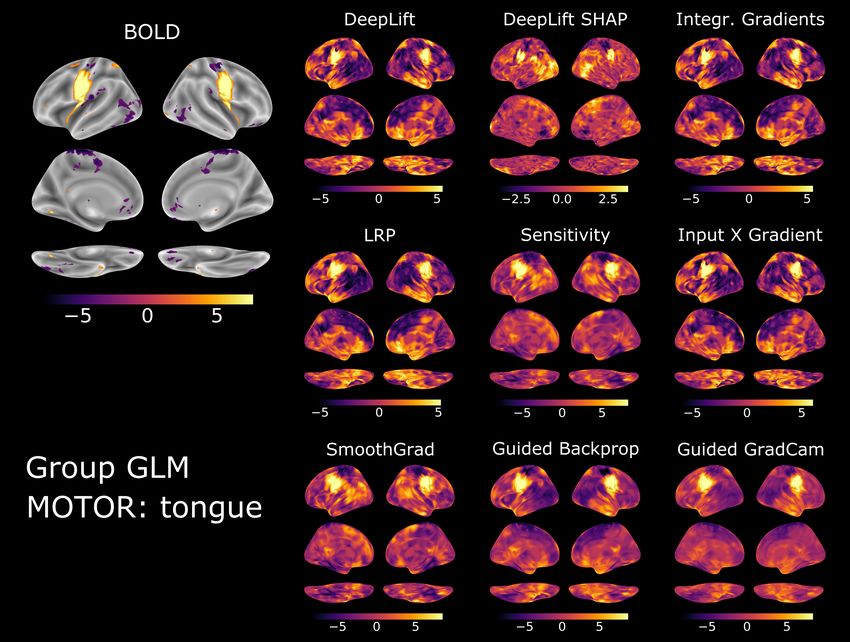
13Figure 5: Attribution faithfulness. We estimated explanation faithfulness of an attribution method by
repeatedly evaluating the models’ test decoding accuracy when occluding different fractions of the input
voxels based on the relevance assigned to them by the attribution method, such that 0% occlusion indicates
that no voxel values were occluded while 50% indicates that the values of all input voxels were occluded
that received the highest 30% of relevance values. For each attribution method and trained model, we
recorded the occlusion rate at which the models’ test decoding accuracy first dropped to chance-level,
indicating that all information has been removed from the data that the model uses to correctly identify
the mental states. A,C,E: DeepLift, DeepLift SHAP, Integrated Gradients, LRP, and InputXGradient
exhibit higher attribution faithfulness than Gradient Analysis, SmoothGrad, Guided Backpropagation,
and Guided GradCam, as the models’ test decoding accuracies decrease more rapidly with increasing
occlusion rates for these methods. Lines indicate mean test decoding accuracies over the ten training runs
of each model and optimization configuration. B,D,F: Accordingly, model test decoding accuracies also
drop to chance-level at lower occlusion rates for these approaches. Scatter points represent model training
runs and black stars indicate that the distribution of occlusion rates is meaningfully different from the
distribution of the DeepLift method (for analysis details, see section 1.6). Colors indicate interpretation
methods.
are specific to the tested model and data by testing how much the explanations change when
the method is applied to a model with the same architecture but random weights (the model
randomization test) or a model trained on a version of the data with randomly permuted labels
(the data randomization test). If the explanations are dependent on the specific parameters of the
model, they should differ between the originally trained models and models with random weights.
If the explanations are similar, however, the attribution method can be considered insensitive to
the studied model and therefore not well-suited to capture the models’ decision process. Similarly,
if the explanations of an attribution method account for the labeling of the data, it should produce
explanations that are different between models model trained on the original dataset and models
trained on a version of the data with randomly shuffled labels. If the explanations are similar,
14Figure 6: Sanity checks for attribution methods. We performed two sanity for each attribution method
by comparing a method’s original attributions to its attributions for the same data when interpreting the
mental state decoding decisions of a model variant trained on a version of the training data with randomized
labels (data randomization test; A, C, E) and model with randomized weights (model randomization test;
B, D, F). If the attributions of an attribution method are sensitive to the characteristics of the input data
and model, its attributions for the original model should be different from its attributions for the model
trained on randomized data as well as the model with random weights (leading to low mutual information
scores). Overall, DeepLift SHAP, Gradient Analysis, Guided Backpropagation, and Guided GradCam
performed better than the other methods in both tests (as indicated by generally lower mutual information
scores), while DeepLift and Integrated Gradients also performed comparably well. Scatter points indicate
mean mutual information for each model training run. Black stars indicate that the distribution of mean
mutual information scores is meaningfully lower than the distribution of the DeepLift method (for analysis
details, see section 1.6). Colors indicate interpretation methods.
however, the attribution method can be considered independent of the labeling of the data and
therefore not well-suited to understand the model’s learned mapping between these labels and the
input data.
In line with the data randomization test, we first trained each model configuration on a version
of its original training dataset with randomly shuffled mental state labels. The models were
able to correctly decode the randomly shuffled mental state labels in their training data after
2, 000 training epochs, achieving decoding accuracies of 85.1%, 98.7%, and 98.4% for the heat-
rejection, MOTOR, and WM datasets respectively (Appendix Fig. A1). Importantly, the models’
validation decoding accuracies were still close to chance (namely, 45.9%, 23.5%, and 25% for the
heat-rejection, MOTOR, and WM datasets respectively; Appendix Fig. A1), indicating that the
models memorized the random associations between labels and training data. When comparing the
attributions of each attribution method for the test mental state decoding decisions of the models
15trained on the randomized and original training data, we found that the attributions of DeepLift
SHAP, Gradient Analysis, SmoothGrad, Guided Backpropagation, and Guided GradCam were
generally more dissimilar between the two models than those of the other attribution methods,
indicating stronger dependence of their attributions on the characteristics of the data.
Similarly, in line with the model parameter randomization test, we also interpreted the test
mental state decoding decisions of a randomly initialized variant of each datasets’ model con-
figuration. As for the data randomization test, we compared the resulting attributions of each
attribution method to the attributions for the originally trained models. Again, DeepLift SHAP,
Gradient analysis, Guided Backpropagation, and Guided GradCam produced attributions that
showed stronger dependence on the characteristics of the analyzed models, when compared to the
other methods, as their attributions for the randomized and originally trained models were more
dissimilar.
3 Discussion
With this work, we provide insights into the explanation performance of prominent types of attribu-
tion methods, namely, sensitivity analyses, backward decompositions, and reference-based attribu-
tions (see section 1.5), in mental state decoding analyses with DL models. To evaluate explanation
performances, we use a diverse set of criteria: First, we evaluate the biological plausibility of the
explanations by comparing them to the results of a standard GLM analysis of BOLD data, which
seeks to identify all voxels whose activity pattern is associated with the mental states. We find
that sensitivity analyses, such Guided Backpropagation, Guided GradCam, Gradient Analysis, and
SmoothGrad, provide explanations that are more similar to the results of the GLM analysis, and
thereby biologically more plausible, than the explanations of the tested backward decompositions
and reference-based attributions. Second, we evaluate whether the explanations accurately cap-
ture the models’ decision process by testing whether they accurately identify all voxels of the input
that the models rely on to identify the mental states. We find that backward decompositions and
reference-based attributions, such as DeepLift, DeepLift SHAP, Integrated Gradients, and LRP,
provide explanations that are more faithful than those of the tested sensitivity analyses. Last, to
test whether the methods’ explanations are in fact sensitive to the analyzed model and data, we
perform two sanity checks for attribution methods (as suggested by Adebayo et al., 2018) and find
that Gradient Analysis, Guided Backpropagation, Guided GradCam, DeepLift SHAP, DeepLift,
and Integrated Gradients perform consistently well in both sanity checks, providing explanations
that are sensitive to the characteristics of the analysed model and data.
3.1 Biological plausibility vs. explanation faithfulness
Our findings demonstrate a gradient between two key characteristics for the interpretation of men-
tal state decoding decisions: attribution methods that provide highly faithful explanations, by
capturing the model’s decision process well, also provide explanations that are biologically less
plausible, because they do not necessarily identify all voxels whose activity patterns are associated
with the mental states, when compared to interpretation methods with less explanation faithful-
ness. To make sense of this finding, it is important to remember that functional neuroimaging
data generally exhibit strong spatial correlations, such that individual mental states are often as-
sociated with the activity of large clusters of voxels. DL models trained to identify these mental
states from neuroimaging data will likely view some of this activity as redundant, as the activity
of a subset of those voxels suffices to correctly identify the mental states. In these situations, any
explanation of an attribution method with perfect faithfulness will not identify all voxels of the
input whose activity is in fact associated with the decoded mental state, but solely the subset of
voxels whose activity the model used as evidence for its decoding decision. Accordingly, attribution
methods with high explanation faithfulness, such as backward decompositions and reference-based
16attributions, do not necessarily produce explanations that align well with the results of a standard
GLM analysis of the BOLD data. By contrast, we found that sensitivity analyses, such as Guided
GradCam, Guided Backpropagation, Gradient Analysis, and SmoothGrad, produce explanations
that are less faithful but more in line with the results of a standard GLM analysis. Sensitivity
analyses are less concerned with identifying the specific contribution of each input voxel to a de-
coding decision and instead focus on identifying how sensitively a model’s decision responds to
(i.e., changes with) the activity of each voxel. With this perspective, sensitivity analyses identify a
broader set of voxels whose activity the model takes into account when decoding the mental state,
resulting in explanations that seem biologically more plausible because the set of identified voxels
is more similar to that of standard analysis approaches for BOLD data, which seek to identify
voxels whose activity pattern is associated with the mental state.
3.2 Recommendations for interpretation methods in mental state de-
coding
Based on these findings, we make a twofold recommendation for the application of attribution
methods in mental state decoding:
If the goal of a mental state decoding analysis is to understand the decision process of the de-
coding model by identifying the parts of the input that are most relevant for the model’s decision,
we generally recommend the application of backward decompositions or reference-based attribu-
tions. In particular, we recommend DeepLift, DeepLift SHAP, and Integrated Gradients because
their explanations have shown overall high faithfulness in our analyses, while also performing well
in the two sanity checks.
By contrast, if the goal of a mental state decoding analysis is to understand the association
between the BOLD data and studied mental states, we recommend the application of sensitivity
analyses, as these have shown to produce explanations with comparably high similarity to the
results of a standard GLM analysis of the data when compared to reference-based attributions
and backward decompositions. Particularly, for CNN models with ReLU activation functions,
we recommend Guided Backpropagation and Guided GradCam as their explanations exhibit the
overall highest similarity to the results of a standard GLM analysis of the BOLD data in our
analyses, while also performing well in the two sanity checks. For models without ReLU activation
functions, we recommend Gradient Analysis and SmoothGrad, as their explanations also have
comparably high similarity to the results of the GLM analysis (especially on the level of individual
subjects), while also performing well in the two sanity tchecks.
3.3 Caution in the interpretation of complex models
Last, we would like to advocate for caution in any interpretation of the mental state decoding
decisions of DL models. DL models have an unmatched ability to learn from and represent complex
data. Accordingly, their learned mappings between input data and decoding decisions can be highly
complex and counterintuitive. For example, recent empirical work has shown that DL methods
trained in mental state decoding analyses can identify individual mental states through voxels that
exhibit meaningfully stronger activity in these states as well as voxels with meaningfully reduced
activity in these states, leading to explanations that assign high relevance scores to voxels that
receive both positive and negative weights in a standard GLM contrast analysis of the same BOLD
data (Thomas et al., 2021a). To understand how a model’s weighting of the input in its decoding
decision relates to the characteristics of the input data, it is therefore essential to compare the
explanations of any attribution method to the results of standard analyses of the BOLD data (e.g.,
with linear models; Friston et al., 1994, Grosenick et al., 2013, Kriegeskorte et al., 2006) as well as
related empirical findings (e.g., as provided by NeuroSynth; Yarkoni et al., 2011).
17Similarly, a wealth of recent empirical work in machine learning research has demonstrated that
DL models are prone to learning simple shortcuts (or confounds) from their training data, which do
not generalize to other datasets (for a detailed discussion, see Geirhos et al., 2020). A prominent
example is a study that trained DL models to identify pneumonia from chest X-rays (Zech et al.,
2018). While the models performed well in the training data, comprising X-rays from few hospitals,
their performance meaningfully decreased for X-rays from new hospitals. By applying attribution
methods to the classification decisions of the trained models, the authors were able to show that
the models learned to accurately identify the hospital system that was used to acquire an X-
ray, in combination with the specific department, allowing them to make accurate predictions on
aggregate by simply learning the overall prevalence rates of these departments. Similar examples
are imaginable in functional neuroimaging, as recently suggested by Chyzhyk et al. (2022) who
state that biomarker models for specific disease conditions could learn to distinguish patients from
controls simply by their generally increased head motion.
For these reasons, we echo a recent call of machine learning researchers to always consider
whether the application of complex models (such as DL models) is necessary to answer the research
question at hand, or whether the application of simpler models, with better interpretability, could
suffice (Rudin, 2019). While we do believe that DL models hold a high promise for mental state
decoding research, e.g., with their ability to learn from large-scale neuroimaging datasets (Schulz
et al., 2022), we also believe that many common mental state decoding analyses, which solely
focus on few mental states in tens to a hundred of individuals, can be well-addressed with simpler
decoding models with better interpretability (e.g., Grosenick et al., 2013, Hoyos-Idrobo et al., 2018,
Kriegeskorte et al., 2006, Michel et al., 2011, Schulz et al., 2020).
We hope that with this work we can provide some insights into the strengths and weaknesses
of prominent interpretation methods in mental state decoding, thereby enabling neuroimaging
researchers to make an informed choice in situations where explanations for the mental state
decoding decisions of DL models are needed.
Acknowledgments. We gratefully acknowledge the support of NIH under No. U54EB020405
(Mobilize), NSF under Nos. CCF1763315 (Beyond Sparsity), CCF1563078 (Volume to Velocity),
and 1937301 (RTML); ARL under No. W911NF-21-2-0251 (Interactive Human-AI Teaming); ONR
under No. N000141712266 (Unifying Weak Supervision); ONR N00014-20-1-2480: Understanding
and Applying Non-Euclidean Geometry in Machine Learning; N000142012275 (NEPTUNE); NXP,
Xilinx, LETI-CEA, Intel, IBM, Microsoft, NEC, Toshiba, TSMC, ARM, Hitachi, BASF, Accen-
ture, Ericsson, Qualcomm, Analog Devices, Google Cloud, Salesforce, Total, the HAI-GCP Cloud
Credits for Research program, the Stanford Data Science Initiative (SDSI), the Texas Advanced
Computing Center (TACC) at The University of Texas at Austin, and members of the Stanford
DAWN project: Facebook, Google, and VMWare. The U.S. Government is authorized to repro-
duce and distribute reprints for Governmental purposes notwithstanding any copyright notation
thereon. Any opinions, findings, and conclusions or recommendations expressed in this material
are those of the authors and do not necessarily reflect the views, policies, or endorsements, either
expressed or implied, of NIH, ONR, or the U.S. Government.
FMRI data for the MOTOR and WM datasets were provided by the Human Connectome
Project (HCP S1200 release), WU Minn Consortium (Principal Investigators: David Van Essen
and Kamil Ugurbil; 1U54MH091657) funded by the 16 NIH Institutes and Centers that support the
NIH Blueprint for Neuroscience Research; and by the McDonnell Center for Systems Neuroscience
at Washington University. FMRI data for the heat-rejection dataset were publicly shared in a
preprocessed format by Kohoutová et al. (2020).
18You can also read