Carbon emissions from land use and land-cover change
←
→
Page content transcription
If your browser does not render page correctly, please read the page content below
Biogeosciences, 9, 5125–5142, 2012
www.biogeosciences.net/9/5125/2012/                                                                 Biogeosciences
doi:10.5194/bg-9-5125-2012
© Author(s) 2012. CC Attribution 3.0 License.

Carbon emissions from land use and land-cover change
R. A. Houghton1 , J. I. House2 , J. Pongratz3,* , G. R. van der Werf4 , R. S. DeFries5 , M. C. Hansen6 , C. Le Quéré7 , and
N. Ramankutty8
1 Woods  Hole Research Center, Falmouth, MA, USA
2 Department  of Geography, Cabot Institute, University of Bristol, Bristol, UK
3 Department of Global Ecology, Carnegie Institution for Science, Stanford, USA
4 Faculty of Earth and Life Sciences, VU University, Amsterdam, The Netherlands
5 Ecology, Evolution, and Environmental Biology, Columbia University, New York, USA
6 Department of Geographical Sciences, University of Maryland, College Park, USA
7 Tyndall Centre for Climate Change Research, University of East Anglia, Norwich, UK
8 Department of Geography, McGill University, Montreal, Canada
* now at: Max Planck Institute for Meteorology, Hamburg, Germany

Correspondence to: R. A. Houghton (rhoughton@whrc.org)

Received: 12 December 2011 – Published in Biogeosciences Discuss.: 19 January 2012
Revised: 10 May 2012 – Accepted: 18 November 2012 – Published: 13 December 2012

Abstract. The net flux of carbon from land use and land-          of uncertainty as they do not account for the errors that result
cover change (LULCC) accounted for 12.5 % of anthro-              from data uncertainty and from an incomplete understand-
pogenic carbon emissions from 1990 to 2010. This net flux         ing of all the processes affecting the net flux of carbon from
is the most uncertain term in the global carbon budget, not       LULCC. Although these errors have not been systematically
only because of uncertainties in rates of deforestation and       evaluated, based on partial analyses available in the litera-
forestation, but also because of uncertainties in the carbon      ture and expert opinion, they are estimated to be on the order
density of the lands actually undergoing change. Further-         of ± 0.5 Pg C yr−1 .
more, there are differences in approaches used to determine
the flux that introduce variability into estimates in ways that
are difficult to evaluate, and not all analyses consider the      1   Definitions and context
same types of management activities. Thirteen recent esti-
mates of net carbon emissions from LULCC are summa-               The sources and sinks of carbon from land use and land-
rized here. In addition to deforestation, all analyses consid-    cover change (LULCC) are significant in the global carbon
ered changes in the area of agricultural lands (croplands and     budget. The contribution of LULCC to anthropogenic car-
pastures). Some considered, also, forest management (wood         bon emissions were about 33 % of total emissions over the
harvest, shifting cultivation). None included emissions from      last 150 yr (Houghton, 1999), 20 % of total emissions in the
the degradation of tropical peatlands. Means and standard de-     1980s and 1990s (Denman et al., 2007), and 12.5 % of to-
viations across the thirteen model estimates of annual emis-      tal emissions over 2000 to 2009 (Friedlingstein et al., 2010).
sions for the 1980s and 1990s, respectively, are 1.14 ± 0.23      The declining fraction is largely the result of the rise in fossil
and 1.12 ± 0.25 Pg C yr−1 (1 Pg = 1015 g carbon). Four stud-      fuel emissions. The net flux of carbon from LULCC is also
ies also considered the period 2000–2009, and the mean and        the most uncertain term in the carbon budget, accounting for
standard deviations across these four for the three decades are   emissions of 1.4 (range: 0.4 to 2.3) Pg C yr−1 in the 1980s;
1.14 ± 0.39, 1.17 ± 0.32, and 1.10 ± 0.11 Pg C yr−1 . For the     1.6 (0.5 to 2.7) Pg C yr−1 in the 1990s (Denman et al., 2007);
period 1990–2009 the mean global emissions from LULCC             and 1.1 ± 0.7 Pg C yr−1 from 2000 to 2009 (Friedlingstein et
are 1.14 ± 0.18 Pg C yr−1 . The standard deviations across        al., 2010).
model means shown here are smaller than previous estimates

Published by Copernicus Publications on behalf of the European Geosciences Union.
5126                                         R. A. Houghton et al.: Carbon emissions from land use and land-cover change

   Several different models, data sets and methods have             changes in carbon stocks are estimated (some are modeled,
been applied to calculate the global net flux of carbon from        others are specified from observations). Approaches also dif-
LULCC. This paper reviews and synthesizes these estimates,          fer in their treatment of environmental change (Sect. 3.4)
providing an update and a more representative range across          and the types of additional management activities considered
the current literature than is presented in either Denman et        (Sect. 4).
al. (2007) or Friedlingstein et al. (2010). The paper discusses         Ideally, land use and land-cover change would be defined
reasons for differences across results, key areas of uncer-         broadly to include not only human-induced changes in land
tainty in estimates, including sources of data and differences      cover, but all forms of land management (e.g., tillage, fer-
in approach, and open questions that lead to priorities for the     tilizer use, shifting cultivation, selective logging, draining of
next steps in constraining emissions from LULCC.                    peatlands, use or exclusion of fire). The reason for this broad
   The flux of carbon from LULCC does not represent the             ideal is that the net flux of carbon attributable to management
total net flux of carbon between land and atmosphere. Un-           is that portion of a terrestrial carbon flux that might qualify
managed terrestrial ecosystems also contribute to changes in        for credits and debits under a post-Kyoto agreement. Besides
the land–atmosphere net flux (Phillips et al., 2008; Lewis          the difficulty in separating management effects from natu-
et al., 2009; Pan et al., 2011). There are large annual ex-         ral and indirect effects (CO2 fertilization, N deposition, and
changes of CO2 between ecosystems (plants and soils) and            the effects of climate change), the ideal of including all land
the atmosphere due to natural processes (photosynthesis, res-       management activities requires more data, at higher spatial
piration) with substantial interannual variability related to       and temporal resolution, than has been practical (or possible)
climate variability. The land is currently a net sink despite       to assemble at the global level. Thus, most analyses of the ef-
LULCC emissions (Canadell et al., 2007; Le Quéré et al.,          fects of LULCC on carbon have focused on the dominant (or
2009). This net sink is likely attributable to a combina-           documentable) forms of management and, to a large extent,
tion of LULCC (e.g., forests growing on abandoned crop-             ignored others.
lands) and the affects of environmental changes on plant                Most analyses include little if any land use (management
growth, such as the fertilizing effects of rising concentra-        within a cover type) despite the effects of land use on ter-
tions of CO2 in the atmosphere and nitrogen (N) deposition,         restrial carbon storage. Several analyses include wood har-
and changes in climate, such as longer growing seasons in           vest and shifting cultivation, but none has included cropland
northern mid-latitude regions. These environmental drivers          management. A reduction in the carbon density of forests as a
affect both managed and unmanaged lands and make attribu-           result of management is defined here as “degradation”. Thus,
tion of carbon fluxes to LULCC difficult. LULCC, in theory,         even sustainable harvests “degrade” forests because the mean
includes only those fluxes of carbon attributable to direct hu-     carbon density of a sustainably logged forest is less than it
man activity and excludes those fluxes attributable to natural      would be if the forest were not logged.
or indirect human effects. In practice, however, attribution is         LULCC also affects climate through emissions of chem-
difficult, in part because of the interactions between direct       ically and radiatively active gases besides CO2 . Further,
and indirect effects. It is difficult to establish how much of      LULCC affects climate through biophysical effects on
the carbon accumulating in a planted forest, for example, can       surface albedo, surface roughness, and evapotranspiration
be attributed to management, as opposed to increasing con-          (e.g., Pongratz et al., 2010). Non-CO2 gases and biophysi-
centrations of CO2 in the atmosphere.                               cal effects are not considered here.
   In this paper the term “land use” refers to management
within a land-cover type, such as forest or cropland. For ex-
ample, the harvest of wood does not change the designation          2   Synthesis of global LULCC estimates
of the land as forest although the land may be temporarily
treeless. “Land-cover change”, in contrast, refers to the con-      Recent estimates of the flux of carbon from LULCC are
version of one cover type to another, for example, the conver-      shown in Fig. 1 and summarized briefly in Table 1. A few of
sion of forest to cropland. The largest emissions of carbon         the estimates are not strictly global but include only tropical
have been from land-cover change, particularly the conver-          regions (DeFries et al., 2002; Achard et al., 2004). Neverthe-
sion of forests to non-forests, or deforestation.                   less, these estimates for the tropics appear to fit within the
   All of the analyses reviewed here have included changes          range of global estimates because the net annual flux of car-
in forest area, and most have included other changes in land        bon from LULCC in regions outside the tropics has been gen-
cover (e.g., natural grassland to pastureland). All of the ap-      erally small compared to tropical fluxes over the last decades
proaches consider changes in the areas of croplands and pas-        (Houghton, 2003). This near neutrality may be misleading,
tures (i.e., areas deforested or reforested) (Sect. 3.1) and the    however. It does not indicate a lack of activity outside the
emissions coefficients (carbon lost or gained per hectare fol-      tropics. Indeed, annual gross sources and sinks of carbon
lowing a change in land cover) (Sects. 3.2 and 3.3). The ap-        from LULCC are nearly as great in temperate and boreal re-
proaches differ, first, in the way changes in area are identified   gions as they are in the tropics (Richter and Houghton, 2011).
and measured; and, second, in the way carbon stocks and             Rates of wood harvest, for example, are nearly the same in

Biogeosciences, 9, 5125–5142, 2012                                                        www.biogeosciences.net/9/5125/2012/
R. A. Houghton et al.: Carbon emissions from land use and land-cover change 5127
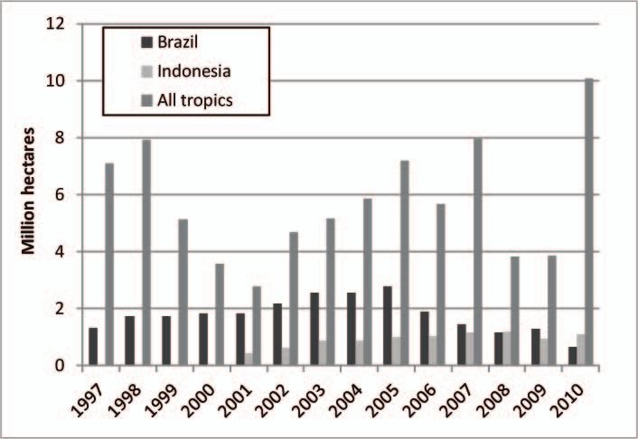
Interannual variability and trends
Satellite-based observations of forest-cover loss and fires
provide one estimate of the interannual variability in defor-
estation rates (Fig. 2). This variability may be driven by com-
modity prices, institutional measures, and climate conditions.
Over the period 2001–2004 clearing rates in the Brazilian
state of Mato Grosso were correlated with soy prices (Morton
et al., 2006). Longer and more extreme dry seasons, allow-
ing for a more effective use of fire, have been linked to higher
clearing rates in Indonesia (van der Werf et al., 2008) and the
Amazon (Aragão et al., 2008). In Southeast Asia the emis-
sions during dry El Niño years may be one or even two or-
ders of magnitude larger than emissions during wet La Niña
years, and at least some of this variability in emissions results
from uses of land tied to climatic variations.
Fig. 1. Recent estimates of the net annual emissions of carbon from Regarding a trend in global emissions from LULCC, no
land use and land-cover change. The closed boxes (DeFries et al., trend stands out in the family of curves in Fig. 1. Those
2002) and circle (Achard et al., 2004) represent 10-yr means for the analyses that extend to 2010 suggest a recent downturn in
1980s or 1990s. net emissions, not statistically significant but consistent with
decreased rates of deforestation reported by the UN’s Food
both regions. The main difference between the two regions is and Agriculture Organization (FAO) in their 2010 Forest Re-
that forests are being lost in the tropics, while forest area has sources Assessment (FRA) and with declining rates of de-
been expanding in Europe, China, and North America. forestation observed in the two countries with the highest
The mean annual net flux of carbon from LULCC based on rates (Fig. 2). However, preliminary results from the FAO &
the thirteen estimates for the 1980s and 1990s is 1.14 ± 0.23 JRC (2012) remote sensing survey suggest the reverse trend:
and 1.12 ± 0.25 Pg C yr−1 , respectively (mean ± standard higher deforestation rates in 2000–2005 than in the 1990s.
deviation across model means). The four estimates for 2000– Reduced rates of deforestation in Brazil appear to have been
2009 yield mean net sources of 1.14 ± 0.39, 1.17 ± 0.32, and offset by increased rates in other South American countries.
1.10 ± 0.11 Pg C yr−1 for the 1980s, 1990s, and 2000–2009, The annual net loss of forest area in the tropics, as
respectively. Only one of these estimates (Houghton, 2010) is reported in the 2010 FRA (FAO, 2010) decreased from
based on recent estimates of deforestation rates (FAO, 2010). 11.55 million ha yr−1 for 1990–2000 to 8.62 million ha yr−1
The three others are forced by scenarios after 2000 or 2005. over the period 2000–2010. In contrast, initial results from
For the longer interval 1990–2009 the mean net flux for all the FAO & JRC (2012) survey show an increase in tropi-
analyses is 1.14 ± 0.18 Pg C yr−1 . cal net deforestation rates from ∼ 8.2 million ha yr−1 during
The standard deviations across model means do not re- the 1990–2000 period to ∼ 10.0 million,ha yr−1 during the
flect the larger uncertainty within each estimate due to uncer- 2000–2005 period. At this point it is unclear which estimate
tainty in data (Sect. 3) and uncertainty in understanding and of deforestation is more accurate. Are the country-based es-
accounting for multiple processes or activities (Sects. 4–5). timates of the FRA subject to large errors (Grainger, 2008),
They also do not fully represent the range around the mod- or is the regularly spaced sample covering 1 % of tropical
eled mean, which is generally in the order of ± 0.5 Pg C yr−1 . forests insufficient to capture the aggregated nature of defor-
Thus they are smaller than the errors presented in Denman estation rates (Steininger et al., 2009)? Over the longer pe-
et al. (2007) and Friedlingstein et al. (2010). A fuller as- riod 1990 to 2005, the means of the two estimates are within
sessment of the uncertainty is presented in Sect. 6 follow- ∼ 10 % of each other.
ing a discussion which identifies the reasons for differences
among these recent estimates. Differences are grouped into 3 Approaches and data
several major categories: data on rates and areas of LULCC
(Sect. 3.1) and data on carbon density of soils and vegeta- 3.1 Changes in area
tion before (Sect. 3.2) and after change (Sect. 3.3), the treat-
ment of environmental change (e.g., CO2 and N fertilization, Three approaches have been used to document changes in the
changes in temperature and moisture) (Sect. 3.4), and the area of ecosystems or changes in land cover: nationally ag-
types of LULCC processes included (or not) (Sects. 4–5). gregated land-use statistics, satellite data on land cover, and
satellite data on fires.
www.biogeosciences.net/9/5125/2012/ Biogeosciences, 9, 5125–5142, 20125128 R. A. Houghton et al.: Carbon emissions from land use and land-cover change
Table 1. Key characteristics of the data sets shown in Fig. 1. Note that several studies provide a range of different estimates of land-use
emissions; the datasets shown in this study were chosen as the ones closest to a bookkeeping approach or to isolate certain processes.
Study Reference Approach LULCC types LULCC source Carbon fluxes Beginning Spatial detail2 Emissions Emissions
(Fig. 1) of accoun- 1920 to 1990 to
ting (AD)1 1999 1999
(Pg C yr−1 ) (Pg C yr−1 )
Achard Achard et al. Bookkeeping De/reforestation, Remote sensing, Actual direct 1990 Explicit (only – 1.10
(2004) model forest degrada- FAO Remote tropics)
tion, peat fires Sensing Survey
Arora Arora and Process model Cropland Ramankutty and Actual direct 1850 Explicit 0.92 1.06
Boer (2010) (CTEM) Foley (1999)
DeFries DeFries et Bookkeeping De/reforestation Remote sensing Actual direct 1982 Explicit (only – 0.90
al. (2002) model tropics)
Houghton Houghton Bookkeeping Ag3 incl. shifting FAO and national Actual direct 1850 Regional 1.21 1.50
(2010) model cultivation in censuses
Latin America/
tropical Asia,
and wood harvest
Piao Piao et al. Process model Ag Ramankutty and Actual direct in- 1900 Explicit 1.31 1.24
(2009) (ORCHIDEE) Foley (1999) (crop- cluding effects of
land), HYDE2.0 observed CO2 and
(pasture), IMAGE climate change
(after 1992)
Pongratz Pongratz et Process model Ag Pongratz et al. Actual direct 800 Explicit 0.90 1.14
LUC al. (2009) (JSBACH) (2008)4
Pongratz Pongratz et Process model Ag Pongratz et al. Actual direct in- 800 Explicit 0.99 1.30
LUC + CO2 al. (2009) (JSBACH) (2008)3 cluding effects of
simulated CO2 and
climate change
Reick Reick et Process model Ag Pongratz et al. Actual direct 800 Explicit 1.03 –
process al. (2010) (JSBACH) (2008)4
Reick book- Reick et Bookkeeping Ag Pongratz et al. Actual direct 800 Explicit 1.34 –
keeping al. (2010) model (2008)4
Shevliakova Shevliakova Process model Ag incl. shifting Hurtt et al. (2006)5 Actual direct 1700 Explicit 1.44 1.31
HYDE/SAGE et al. (2009) (LM3V) cultivation in
tropics, and
wood harvest
Shevliakova Shevliakova Process model Ag incl. shifting Hurtt et al. (2006)6 Actual direct 1700 Explicit 1.28 1.07
HYDE et al. (2009) (LM3V) cultivation in
tropics, and
wood harvest
Strassmann Strassmann Process model Ag, urban HYDE2.0 adjusted Actual direct 1700 Explicit 1.39 0.75
et al. (2008) (LPJ in BernCC)
Stocker Stocker et Process model Ag, urban HYDE3.1 adjusted Actual direct 10 000 BC Explicit 1.31 0.93
al. (2011) (LPJ in BernCC,
updated since
Strassmann,
2008)
Van Minnen Van Minnen Process model Ag, wood HYDE (ag), Actual direct in- 1700 1.16 1.33
et al. (2009) (IMAGE2) harvest IMAGE2 (w.h.) cluding effects of
CO2 , climate
change, and
management4
Zaehle Zaehle et al. Process model Ag, urban Hurtt et al. (2006) Actual direct 1700 1.32 0.97
(2011) (O-CN)
1 I.e., legacy emissions of earlier time periods not considered.
2 Unless otherwise noted, studies considered all land area.
3 “Ag” stands for changes in land cover caused by expansion or abandonment of agricultural area; agriculture includes both cropland and pasture.
4 Based on SAGE cropland and SAGE pasture with rates of pasture changes from HYDE, preferential allocation of pasture on natural grassland.
5 Based on SAGE cropland and HYDE pasture, proportional scaling of natural vegetation.
6 Based on HYDE cropland and HYDE pasture, proportional scaling of natural vegetation.
7 An “autonomous growth factor” approximates increase in plant productivity due to nitrogen fertilization and forest management changes.
Biogeosciences, 9, 5125–5142, 2012 www.biogeosciences.net/9/5125/2012/R. A. Houghton et al.: Carbon emissions from land use and land-cover change 5129
tions about whether agricultural expansion occurs at the ex-
pense of grasslands or forests, and where these changes take
place, as in the SAGE (Ramankutty and Foley, 1999) and
HYDE (Klein Goldewijk, 2001) data sets. The distinctions
are important because different locations have different car-
bon stocks, and the carbon flux resulting from LULCC de-
pends on assumptions about both land-cover type and carbon
stocks before and after change. Remote sensing-based infor-
mation on recent land-cover change (see next Sect. 3.1.2) can
also be combined with regional tabular statistics from FAO
to reconstruct spatially explicit land-cover changes cover-
ing more than the satellite era (Ramankutty and Foley, 1999;
Klein Goldewijk, 2001; Pongratz et al., 2008). The FAO data
sets (FRA and FAOSTAT) have also been used in combina-
tion to estimate rates of deforestation for shifting cultivation
Fig. 2. Interannual variation in rates of deforestation in Brazil (dark (Houghton and Hackler, 2006), a rotational use of land with
bars) (INPE, 2010) in Indonesia (light bars) (Hansen et al., 2009 repeated clearing and subsequent regrowth of fallow forests.
and updated) and in all tropical forests (van der Werf et al., 2010). The FAO data rely on reporting by individual countries.
The values for Brazil include only the loss of intact forest within They are more accurate for some countries than for oth-
the Legal Amazonia, while for Indonesia they include the loss of ers and are not without inconsistencies and ambiguities
all forests meeting the definition of 30 % cover and 5 m-tall canopy (Grainger, 2008). Revisions in the reported rates of deforesta-
at 60 m spatial resolution (approximately half of these Indonesian
tion from one 5-yr FRA assessment to the next may be sub-
forests are intact). The pantropical estimates are based on burned
stantial due to different methods or data being used. FAO es-
area and active fire detections in forested areas.
timates of deforestation rates over the last few decades have
been reduced by incorporating satellite data (FAO, 2001,
3.1.1 Nationally aggregated land-use statistics 2006, 2010).
Data on historical land-area change prior to the FAO re-
Historic land-use change data sets have been constructed ports have been obtained from a variety of national and inter-
based on aggregated, non-spatial data on LULCC, as re- national historical narratives as well as population and socio-
ported in national and international statistics. The FAO pro- economic data, and national land-use statistics. Agricultural
vides two data sets that have been used to estimate changes expansion has been distributed spatially on the basis of pop-
in land cover over recent decades. One data set (FAOSTAT, ulation densities (Klein Goldewijk, 2001) and hindcasting
2009) reports annual areas in croplands and pastures from of the current distribution of agricultural lands (Ramankutty
1961. The other data set (Forest Resource Assessments, and Foley, 1999). Data sets have been updated and extended
FRAs; FAO 2001, 2006, 2010) provides information on for- to the pre-industrial past (Pongratz et al., 2008; Klein Gold-
est area and carbon stocks from 1990 to 2010. Both data sets ewijk et al., 2011).
include nearly all countries and, hence, enable global esti- Two spatial data sets, in particular, have been used in most
mates to be calculated. The data are not spatially explicit, of the analyses included in Fig. 1: the SAGE data set, includ-
however, and do not specify the cover type from which con- ing cropland areas from 1700–1992 (Ramankutty and Foley,
version happens. They require independent data or allocation 1999), and the HYDE data set, including both cropland and
rules to assign changes in forest or cropland area to or from pasture areas (Klein Goldewijk, 2001). The difference in us-
particular ecosystem types (with specific carbon densities) ing these two data sets accounts for about a 15 % difference
and to particular spatial locations. The FAOSTAT data re- in flux estimates over the period 1850–1990 (Shevliakova et
port areas of cropland and pasture annually, thus providing al., 2009) and 1920–1990 (Fig. 1; Table 1). Other recent data
the basis for calculating annual rates of land-cover change. sets, such as the ones compiled by Hurtt et al. (2006) and
However, these changes are net changes, not gross changes. Pongratz et al. (2008), are based on combinations of SAGE,
Net changes in land cover underestimate gross sources and HYDE and Houghton data sets, including updates.
sinks of carbon that result from simultaneous clearing for,
and abandonment of, agricultural lands, for example, under- 3.1.2 Satellite data on land cover
estimating areas of secondary forests and their carbon sinks.
Approaches based on these FAO data assign deforested A complementary approach for estimating LULCC is to use
areas to either croplands or pastures, as in the Houghton a time series of satellite data to estimate the spatio-temporal
data set (Houghton, 2003). This data set is not spatially ex- dynamics of change. In general, satellite data alleviate the
plicit but aggregates country data into regional data. Spa- concerns of bias, inconsistency, and subjectivity in country
tially explicit approaches based on FAOSTAT make assump- reporting (Grainger, 2008). Depending on the spatial and
www.biogeosciences.net/9/5125/2012/ Biogeosciences, 9, 5125–5142, 20125130 R. A. Houghton et al.: Carbon emissions from land use and land-cover change
temporal resolution, satellite data can also distinguish be- ity for integrating Landsat-scale change to annual time-steps
tween gross and net losses of forest area. However, increases (Broich et al., 2011b).
in forest area are more difficult to observe with satellite data In general, moderate spatial resolution imagery is limited
than decreases because forest growth is a more gradual pro- in tropical forest areas by data availability. Currently Landsat
cess. Furthermore, although satellite data are good for mea- is the only source of data at moderate spatial resolution avail-
suring changes in forest area, they have generally not been able for tropical monitoring, but to date an uneven acquisition
used to distinguish the types of land use following deforesta- strategy among bioclimatic regimes limits the application of
tion (e.g., croplands, pastures, shifting cultivation). Excep- generic biome-scale methods with Landsat. No other system
tions include the regional studies by Morton et al. (2006) and has the combination of (1) global acquisitions, (2) historical
Galford et al. (2008). record, (3) free and accessible data, and (4) standard terrain-
Satellite-based methods include both high-resolution corrected imagery, along with robust radiometric calibration,
sample-based methods and wall-to-wall mapping analyses. that Landsat does. Future improvements in moderate spatial
Sample-based approaches employ systematic or stratified resolution tropical forest monitoring can be obtained by in-
random sampling to quantify gains or losses of forest area creasing the frequency of data acquisition.
at national, regional and global scales (Achard et al., 2002, The primary weakness of satellite data is that they are not
2004; Hansen et al., 2008a, 2010). Systematic sampling pro- available before the satellite era (Landsat began in 1972).
vides a framework for forest area monitoring. The UN-FAO Long time series are required for estimating legacy emis-
Forest Resource Assessment Remote Sensing Survey uses sions of past land-use activity (Sect. 3.3). Although maps, at
samples at every latitude/longitude intersection to quantify varying resolutions, exist for many parts of the world, spatial
biome and global-scale forest change dynamics from 1990 to data on land cover and land-cover change became available
2005 (FAO & JRC, 2012). Other sampling approaches strat- at a global level only after 1972, at best. In fact, there are
ify by intensity of change, thereby reducing sample inten- many gaps in the coverage of the Earth’s surface before 1999
sity. Achard et al. (2002) provided an expert-based stratifica- when the first global acquisition strategy for moderate spatial
tion of the tropics to quantify forest cover loss from 1990 to resolution data was undertaken with the Landsat Enhanced
2000 using whole Landsat image pairs. Hansen et al. (2008a, Thematic Mapper Plus sensor (Arvidson et al., 2001). The
2010) employed MODIS data as a change indicator to strat- long-term plan of Landsat ETM+ data includes annual global
ify biomes into regions of homogeneous change for Landsat acquisitions of the land surface, but cloud-cover and pheno-
sampling. logical variability limit the ability to provide annual global
Sampling methods such as described above provide re- updates of forest extent and change. The only other satellite
gional estimates of forest area and change with uncer- system that can provide global coverage of the land surface
tainty bounds, but they do not provide a spatially explicit at moderate resolution is the ALOS PALSAR radar instru-
map of forest extent or change. Wall-to-wall mapping does. ment, which also includes an annual acquisition strategy for
While coarse-resolution data sets (> 4 km) have been cali- the global land surface (Rosenquist et al., 2007). However,
brated to estimate wall-to-wall changes in area (DeFries et large area forest-change mapping using radar data has not
al., 2002), recent availability of moderate spatial resolution yet been implemented.
data (< 100 m), typically Landsat imagery (30 m), allows
a more finely resolved approach. Historical methods rely 3.1.3 Satellite data on fires
on photointerpretation of individual images to update forest
cover on annual or multi-year bases, such as with the Forest A third approach, applied so far only in tropical forests, uses
Survey of India (Global Forest Survey of India, 2008) or the satellite detection of fires in forests to estimate emissions
Ministry of Forestry Indonesia products (Government of In- from deforestation based on the assumption that a large pro-
donesia/World Bank, 2000). Advances in digital image pro- portion of land clearing in the tropics is by fire (van der Werf
cessing have led to the operational implementation of map- et al., 2010). The approach provides an estimate of gross
ping annual forest-cover loss with the Brazilian PRODES forest loss but does not identify LULCC where fire is ab-
(INPE, 2010) and the Australian National Carbon Account- sent, for example, wood harvest. Nor does it distinguish be-
ing products (Caccetta et al., 2007). These two systems rely tween intentional deforestation fires and escaped wildfires.
on cloud-free data to provide single-image/observation up- The approach combines estimates of burned area (Giglio et
dates on an annual basis. Persistent cloud cover has limited al., 2010) with complementary observations of fire occur-
the derivation of products in regions such as the Congo Basin rence (Giglio et al., 2003). It makes assumptions about how
and Insular Southeast Asia (Ju and Roy, 2008). For such ar- much fire is for clearing. At province or country level, clear-
eas, Landsat data can be used to generate multi-year esti- ing rates calculated this way capture up to about 80 % of the
mates of forest-cover extent and loss (Hansen et al., 2008b; variability and also 80 % of the total clearing rates found by
Broich et al., 2011a). For regions experiencing forest change other approaches (Hansen et al., 2008a; INPE, 2010). One
at an agro-industrial scale, MODIS data provide a capabil- advantage of the fire-counting approach is that it allows for
an estimate of interannual variability (see Sect. 2.1, above).
Biogeosciences, 9, 5125–5142, 2012 www.biogeosciences.net/9/5125/2012/R. A. Houghton et al.: Carbon emissions from land use and land-cover change 5131
3.2 Carbon stocks and changes in them: data sources cover a wide spatial area, and thus can better capture the spa-
and modeling approaches tial and temporal variability in aboveground carbon density.
By matching carbon density to the actual area of forest be-
Three approaches have been used to estimate carbon den- ing deforested, this approach has the potential to increase the
sity (Mg C ha−1 ) and changes in carbon density as a re- accuracy of flux estimates, especially in tropical areas where
sult of LULCC: inventory-based estimates of carbon density variability of carbon density is high, and data availability is
used with bookkeeping model approaches to tracking change poor.
in carbon pools, satellite-based estimates of carbon density The capability of measuring changes in carbon density
used with a variety of model approaches, and process-based through monitoring is in its infancy, but such a capability
vegetation models that internally calculate biomass density would enable a method for estimating carbon sources and
and changes in carbon pools based on environmental drivers. sinks that is more direct than identifying disturbance first,
and then assigning a carbon density or change in carbon
3.2.1 Inventory-based estimates density (Houghton and Goetz, 2008). The approach would
require models and ancillary data to calculate changes in
Inventory methods use ground-based measurements reported soil, slash, and wood products. Furthermore, estimation of
in forestry and agricultural statistics and the ecological lit- change, by itself, would not distinguish between deliber-
erature. Inventory data are available on the carbon density ate LULCC activity and indirect anthropogenic or natural
of vegetation and soils in different ecosystem types, and the drivers. Nevertheless, estimation of change in aboveground
changes in them following disturbance or management. Ex- carbon density has clear potential for improving calculations
tensive data are available in many temperate regions, but data of sources and sinks of carbon.
are more limited in tropical regions. These data on carbon
density are combined with data on changes in land cover to 3.2.3 Modeled estimates
track changes in carbon using empirical bookkeeping mod-
els. These models track areas of change and types of change, Process-based ecosystem models calculate internally the car-
and use standard growth and decomposition curves to track bon density of vegetation and soils in different types of
changes in carbon pools. For example, conversion of native ecosystems based on climate drivers and other factors within
vegetation to cropland (i.e., cultivation) causes 25–30 % of the models (see e.g., McGuire et al., 2001; Friedlingstein et
the soil organic carbon in the top meter to be lost (Post and al., 2006 for model intercomparisons). These models sim-
Kwon, 2000; Guo and Gifford, 2002; Murty et al., 2002). ulate spatial and temporal variations in ecosystem structure
The conversion of lands to pastures, generally not cultivated, and physiology. Models differ in detail with respect to num-
typically has less of an effect on soil carbon. This tracking ber of plant functional types (PFT’s) (e.g., tropical evergreen
approach is appropriate for non-spatial models. It assigns an forest, temperate deciduous forest, grassland) and number of
average carbon density for biomass and for soils to all land carbon pools (e.g., fast and slow decaying fractions of soil
within a small number of particular ecosystem types (e.g., de- organic matter). They simulate changes in carbon density by
ciduous forest, grassland). Considerable uncertainty arises accounting for disturbances and recovery, whether natural or
because, even within the same forest type, the spatial vari- anthropogenic.
ability in carbon density is large, in part because of variations Net primary productivity is simulated in these ecosystem
in soils and microclimate, and in part because of past distur- models as a function of the vegetation or PFT, local radia-
bances and recovery. Furthermore, literature-based estimates tive, thermal, and hydrological conditions of the soil and the
of carbon density are representative of a specific time and do atmosphere, as well as the atmospheric composition. Soil or-
not capture changes in carbon density that may occur from ganic matter decomposition is commonly controlled by tem-
environmental effects such as natural disturbance, pollution, perature and soil moisture. The ecosystem models, there-
CO2 fertilization and climate change. fore, respond to changes in climate and atmospheric compo-
sition. The models emphasize different aspects of ecosystem
3.2.2 Satellite-based estimates dynamics, with some accounting for competition between
PFTs, nutrient limitation, and natural disturbances.
New satellite techniques are being applied to estimate above- Anthropogenic land-cover change is usually prescribed
ground carbon densities. Examples of mapping aboveground from maps based on spatially explicit data sets, such as
carbon density over large regions include work with MODIS HYDE or SAGE (Sect. 3.1). The land-cover change leads
(Houghton et al., 2007), multiple satellite data (Saatchi et al., to a change in the fraction of PFT that is present at that lo-
2007, 2011), radar (Treuhaft et al., 2009), and lidar (Baccini cation, and a subsequent re-allocation of carbon to the at-
et al., 2012) (see Goetz et al., 2009, for a review). While the mosphere, to soil and to product pools, where carbon de-
accuracy is lower than site-based inventory measurements composes with different turnover rates. Models differ widely
(inventory data are generally used to calibrate satellite algo- with respect to implementation of land use (management),
rithms), the satellite data are far less intensive to collect, can e.g., wood harvest, grazing, and other management activities.
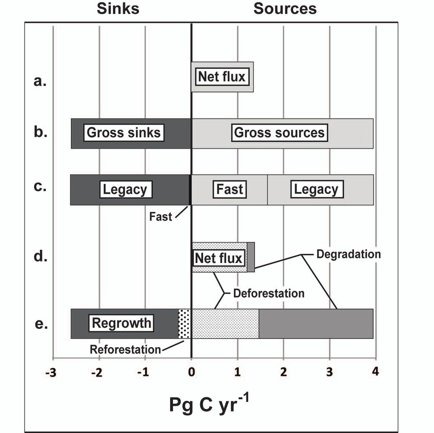
www.biogeosciences.net/9/5125/2012/ Biogeosciences, 9, 5125–5142, 20125132 R. A. Houghton et al.: Carbon emissions from land use and land-cover change Regrowth follows abandonment of managed land. In the ab- to the completeness of conversion; multiple fire events are sence of detailed information on land conversion, specific al- needed for complete removal of biomass, resulting in high location rules have to be applied to determine which natural fire persistence (Morton et al., 2008) and high combustion vegetation type is reduced or expanded when managed land completeness (van der Werf et al., 2010). expands or is abandoned. Common rules include a propor- Over the period 1997–2010, average fire emissions from tional reduction of natural vegetation (Pitman et al., 2009) deforestation and degradation in the tropics with this ap- and the preferential allocation of pasture to natural grassland proach were 0.4 Pg C yr−1 , with considerable uncertainty. (Pongratz et al., 2008). Fires from peatlands added another 0.1 Pg C yr−1 (Sect. 5.1), In contrast to bookkeeping models that specify changes in for a total of 0.5 Pg C yr−1 . This estimate does not include soil and vegetation carbon density based on a limited num- emissions from respiration and decay of residual plant mate- ber of observations, process-based models calculate vegeta- rial and soils, nor does it account for changes in land use that tion and soil carbon density and changes in them for a greater do not rely on fire. To account for decay, fire emissions were number of PFT’s. Furthermore, both net primary production doubled (Barker et al., 2007; Olivier et al., 2005), yielding an (NPP) and decomposition vary over time in response to cli- annual average estimate of ∼ 1 Pg C yr−1 , in line with global mate change and, if included in the model, to the fertilizing model-based estimates (Fig. 1), (although none of the global effects of changes in atmospheric CO2 and N. The process- model-based estimates included emissions from drained and based models can therefore reflect much greater spatial and burned peatlands). Future research is needed to determine the temporal variability in carbon density and response to en- exact ratio between fire and decay, something that is highly vironmental conditions than bookkeeping models, but their variable depending on post-deforestation land use. The main modeled carbon stocks may differ markedly from observa- advantage of using fire to study deforestation emissions is tions. that the fire emissions can be constrained using emitted car- The sensitivity of carbon fluxes to the choice of model bon monoxide, which is routinely monitored by satellites and has been assessed in two studies. McGuire et al. (2001) ap- provides a much larger departure from background condi- plied four different process-based ecosystem models to sim- tions than emitted CO2 (e.g., van der Werf et al., 2008). ilar data on cropland expansion; resulting land-cover emis- The approach underestimates carbon emissions for uses of sions ranged from 0.6 to 1.0 Pg C yr−1 for the 1980s or from land, such as wood harvest, that do not involve fire; it can 56 to 91 Pg C for 1920–1992. Reick et al. (2010) applied potentially overestimate LULCC carbon emissions if it acci- a process-based model (JSBACH) and a bookkeeping ap- dentally includes natural fires (i.e., part of the natural cycle proach (based on Houghton, 2003) to identical LULCC data of fire and regrowth not subsequently resulting in an anthro- and found that land-cover emissions were 40 % higher for the pogenic LULCC). Changes in forest area as determined from bookkeeping approach than the process-based approach (153 satellite data are not clearly attributable to management, as vs. 110 Pg C for 1850–1990) (see Fig. 1 and Table 1). The opposed to natural, processes. By definition, the sources and difference could be attributed almost entirely to differences sinks of carbon for LULCC should not include the sources in soil carbon changes; the bookkeeping model assumed a and sinks from natural disturbances and recovery. The latter 25 % loss of soil carbon to the atmosphere with cultivation are part of the residual terrestrial net flux. Fires, in particu- of native soils, while the process-based model calculated soil lar, are difficult to attribute to natural processes, indirect ef- carbon changes based on changes in NPP and the input of fects (e.g., anthropogenic climate change), or direct manage- organic material associated with the change in land use. Dif- ment. The point here is that natural disturbances and recov- ferences in the way models treat environmental change is ad- ery may be accidentally included in satellite-based analyses dressed in Sect. 3.4. of LULCC. 3.2.4 Fires-based estimates 3.3 The treatment of delayed (legacy) fluxes When satellite-based observations of fires in tropical forests In addition to the areas affected annually by LULCC and the are used to estimate rates of deforestation, the associated carbon densities of the lands affected, rates of decomposition emissions of carbon are estimated by combining the fire- and rates of recovery following LULCC vary among mod- determined clearing rates with modeled carbon densities (van els. Lags in emissions and sinks of carbon are not treated der Werf et al., 2010). Aboveground carbon densities are consistently, adding to the differences among flux estimates. modeled (as in Sect. 3.2.3, above), but the changes in car- To help illustrate the effects of these components, it is help- bon density as a result of fire are calculated differently from ful to distinguish the net annual flux of carbon from the the methods described above. The fraction of aboveground gross sources and sinks that comprise it. Houghton’s anal- biomass lost to fire is based on a pre-defined range of com- ysis (Fig. 1) is used as an illustration. The mean net flux of bustion completeness using literature values and a scaling carbon from LULCC by this estimate was a global source of factor based on the fire persistence. This metric captures how 1.1 Pg C yr−1 over the period 2000–2009. Gross sources and many times a fire is seen in the same grid cell, and is related sinks of carbon were about three times greater (Fig. 3a and b) Biogeosciences, 9, 5125–5142, 2012 www.biogeosciences.net/9/5125/2012/
R. A. Houghton et al.: Carbon emissions from land use and land-cover change 5133
and probably underestimated because deforestation (based
on FAO FRA data) was driven by net (rather than gross)
changes in forest and agricultural area, thereby underesti-
mating agricultural abandonment and the area of secondary
forests.
Instantaneous emissions occur in the year of the distur-
bance, e.g., due to fire and rapid decomposition of carbon
pools. Legacies result from the longer-term losses of carbon
from dead biomass, soils, and forest products and the longer-
term uptake of carbon in regrowing secondary forests. While
the differences do not affect cumulative emissions over a
long time period, short-term emission fluxes can vary sub-
stantially (Ramankutty et al., 2007).
The fraction and fate of biomass removed as a result of
LULCC varies depending on the land use following clear-
ing (Morton et al., 2008). Mechanized agriculture gener-
ally involves more complete removal of above- and below-
ground biomass than clearing for small-scale farming or pas-
ture. For example, in the southern Amazon state of Mato
Grosso, estimated average emissions for 2001–2005 were
116 Mg C ha−1 when forests were converted to cropland and
94 Mg C ha−1 when they were converted to pasture (DeFries
et al., 2008). Incorporating post-clearing land cover in esti-
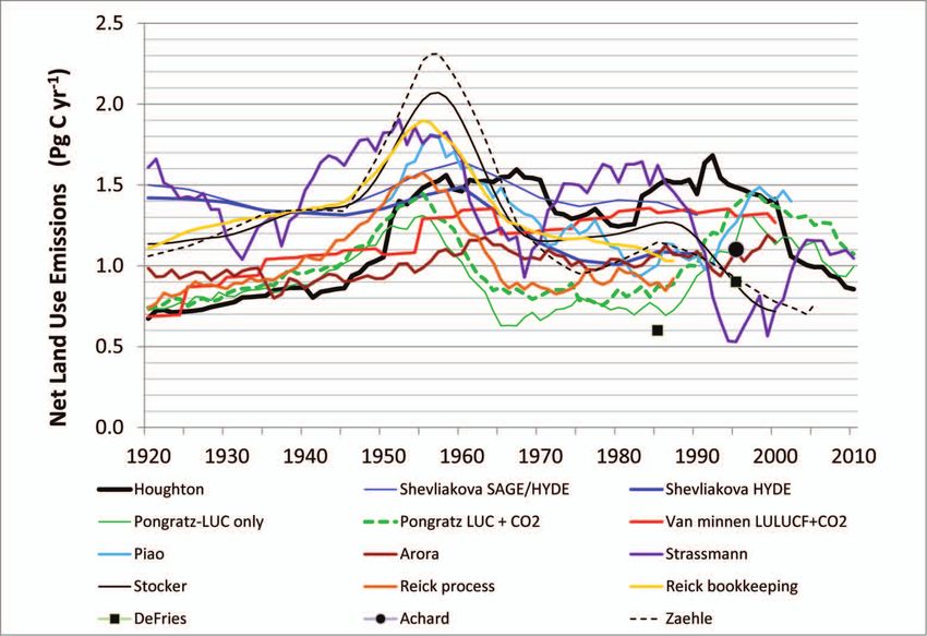
mating carbon emissions from land-use change will reduce Fig. 3. Mean annual net (a) and gross (b) sources and sinks of
uncertainties (Galford et al., 2010). carbon 2000-2009 attributable to LULCC (from Houghton’s anal-
The existence of delayed fluxes implies that estimates of ysis as reported in Friedlingstein et al., 2010). Units are Tg C yr−1 .
current fluxes must include data on historical land-cover ac- “Legacy” in 2c refers to the sinks (regrowth) and sources (decompo-
tivities and associated information on the fate of cleared sition) from activities carried out before 2000; “Fast” in 2c refers to
carbon. However, such historical data are not included in sinks and sources resulting from the current year’s activity. Most of
all analyses, especially in studies using remote-sensing data the net flux (2d) is attributable to deforestation, with a smaller frac-
where information is available only since the 1970s at best tion attributable to forest degradation. The reverse is true for gross
(DeFries et al., 2002; Archard et al., 2004). This leads to the emissions 2e): degradation accounts for more of the gross emissions
than deforestation. Most of the gross annual sink (2e) is attributable
question of how far back in time one needs to conduct analy-
to regrowth (in logged forests or the fallows of shifting cultivation),
ses in order to estimate current emissions accurately, or, alter-
with a smaller sink attributable to reforestation (an increase in forest
natively, how much current emissions are underestimated by area following abandonment of agricultural land.
ignoring historical legacy fluxes. The answer depends on var-
ious factors including: (1) the rates of past clearing; (2) the
fate of cleared carbon (including combustion completeness, 70 % going to slash pools, 8 % to product pools, and 2 % to
repeat fires, etc.); (3) the fate of product and slash pools; and elemental carbon, and calculated annual actual fluxes from
(4) the rate of forest growth following harvest or agricultural 1961 to 2003. When they repeated the analysis ignoring his-
abandonment. If the rate of clearing in historical time peri- torical land use prior to 1981, they underestimated the 1990–
ods is negligible, it is clear that legacy fluxes will be small. 1999 emissions by 13 %, and, while ignoring data prior to
If most of the carbon cleared during previous land uses is 1991, underestimated emissions by 62 %. However, if the as-
burned (and immediately lost to the atmosphere during those sumption of the fate of cleared carbon was altered to 70 %
historical times), legacy fluxes will also be small. However, burned annually and 20 % left as slash, the underestimated
if a significant amount of historically cleared carbon remains emissions for ignoring pre-1981 data and pre-1991 data de-
in the soil to decompose or is turned into products which creased to 4 % and 21 %, respectively.
oxidize slowly, legacy fluxes will be high today (unless soil Globally, the contribution of instantaneous and legacy
decomposition rates or product oxidation rates are also high). fluxes to the mean net flux 2000–2009 is shown in Fig. 3c. In-
The same reasoning applies to rates of growth of secondary stantaneous (fast) and legacy effects contribute about equally
forests. to gross emissions in this study. In contrast, gross sinks are
Ramankutty et al. (2007) explored these issues using a sen- almost entirely legacy fluxes, resulting from the uptake of
sitivity analysis in the Amazon. Their “control” study used carbon by secondary forests established in previous years fol-
historical land-use information since 1961, assumed a con- lowing harvests and agricultural abandonment.
stant annual fraction of 20 % of cleared carbon being burned,
www.biogeosciences.net/9/5125/2012/ Biogeosciences, 9, 5125–5142, 20125134 R. A. Houghton et al.: Carbon emissions from land use and land-cover change
Legacies affect the current sources and sinks of carbon strength of this effect depends on the atmospheric CO2 con-
not only through the accumulation of decaying pools and centration as well as the area of forest lost. This effect has
secondary forests, but through the current distribution of been called the “loss of additional sink capacity” (Pongratz
biomass density. Forests with a long history of use, for ex- et al., 2009), or, when delayed emissions from past land use
ample, may have lower biomass densities than undisturbed are included, the “net land-use amplifier effect” (Gitz and
forests, and the emissions of carbon from degraded forests, Ciais, 2003) and “replaced sinks/sources” (Strassmann et al.,
when they are deforested, will be lower than the emissions 2008). Estimates vary from ∼ 4 Pg C for 1850–2000 (Pon-
from intact forests. In this respect fluxes of carbon from gratz et al., 2009) and 8.5 Pg C for 1950–2100 (Sitch et al.,
LULCC are sensitive to the start times of analyses (i.e., the 2005), to ∼ 0.2 Pg C yr−1 for 1990–2000 (Strassmann et al.,
history of previous use) (Hurtt et al., 2011). 2008) and 125 Pg C for 1700–2100 (Gitz and Ciais, 2003),
All the process model studies in Fig. 1 and Table 1 and the including delayed emissions.
Houghton approach include legacy fluxes, while the satellite Estimates differ with respect to assumptions about climate
approach of DeFries et al. (2002) and Achard et al. (2004) do and the atmospheric CO2 concentrations. Some estimates
not. Another approach with satellite data is to calculate the determine the LULCC flux under a static climate (e.g., a
“committed” flux (Fearnside, 1997; Harris et al., 2012). The pre-industrial climate); others determine it under a realis-
committed flux counts all emissions related to a specific land- tically evolving climate driven by anthropogenic emissions
use activity; that is, both instantaneous and delayed emis- and natural variability. Because effects are partly compensat-
sions that will occur in the future, over a given time horizon. ing (e.g., deforestation under increasing CO2 leads to higher
It can thus be calculated without knowing historical land- emissions because CO2 fertilization has increased carbon
use changes. This approach may be useful in some cases, stocks, but regrowth is also stronger under higher CO2 con-
e.g., for comparing alternative land-use activities with regard centrations), a CO2 fertilization effect is not likely a major
to their total anticipated emissions (Fearnside, 1997). Actual factor in differences among emission estimates (McGuire et
and committed approaches have different intended uses, and al., 2001). Over the industrial era, the combined effects of
they should not be directly compared, as demonstrated by changes in climate and atmospheric composition by one es-
Ramankutty et al. (2007). timate have increased LULCC emissions by about 8 % (Pon-
gratz et al., 2009; Fig. 1, Table 1). Zaehle et al. (2011) in-
3.4 Treatment of environmental change cluded the effects of N deposition, and there are doubtlessly
other interactions, as well, between environmental changes
Bookkeeping models use rates of growth and decay derived and management, making comparisons and attribution diffi-
from the scientific literature, selecting fixed rates for differ- cult.
ent types of ecosystems. Process-based models, on the other Note that nearly all of the estimates in Fig. 1 exclude the
hand, simulate these processes as a function of climate vari- fluxes of carbon driven by environmental effects on natural
ability and trends in atmospheric CO2 . Thus, a comparison vegetation. Both managed and natural ecosystems may be re-
of land-use effects from the two types of models will be con- sponding similarly to environmental changes, but in this re-
founded by environmental effects. Further, sinks attributable view only those lands affected by LULCC, and only those
to LULCC, as calculated with bookkeeping models, will not fluxes attributable to LULCC, have been included, to the ex-
necessarily be equivalent to sinks measured by successive tent possible.
forest inventories, which include environmental effects.
To separate the effects of environmental change, several
process-based modeling analyses have carried out runs with 4 Additional LULCC processes not included in all
and without fixed climate, CO2 , and land use. For exam- analyses
ple, Pongratz et al. (2009) carried out runs with and with-
As discussed above (Sect. 3), variability between the esti-
out changing CO2 concentrations. While some model results
mates of flux from LULCC results, in large part, because of
shown in Table 1 include climate and CO2 effects on areas
differences in data used to estimate deforestation rates and
subject to LULCC (Piao et al., 2009; Van Minnen et al.,
carbon density (see also Houghton, 2005, 2010). The vari-
2009), most process-based models were run with and without
ability also results from the types of land use included. All of
LULCC, and the difference between the two runs was taken
the analyses reviewed here have included changes in the land
to yield the net effects of LULCC. The exercise is not per-
area of forests, cropland and pastures. Additional LULCC ac-
fect, because the effects of CO2 fertilization on undisturbed
tivities, included in some but not all of the analyses in Fig. 1,
forests may differ, for example, from the effects on crop-
are outlined in this section.
lands or on secondary forests recovering from agricultural
abandonment. Furthermore, the woody biomass of forests
has a greater capacity than the herbaceous biomass of crops
and grasslands to store carbon, and this capacity is reduced
as forests are converted to non-forest lands. In models, the
Biogeosciences, 9, 5125–5142, 2012 www.biogeosciences.net/9/5125/2012/R. A. Houghton et al.: Carbon emissions from land use and land-cover change 5135
4.1 Forest management: Wood harvest and shifting dressed the potential for management to sequester carbon,
cultivation but fewer studies have tried to estimate past or current car-
bon sinks. One analysis for the US suggests a current sink
Few of the global models deal with any kind of manage- of 0.015 Pg C yr−1 in croplands (Eve et al., 2002), while a
ment within forest areas, even though this can lead to sub- recent assessment for Europe suggests a small net source
stantial degradation of forest carbon stocks. Selective log- or near-neutral conditions (Ciais et al., 2010; Kutsch et al.,
ging in Amazonia, for example, added 15–19 % to the emis- 2010). In Canada, the flux of carbon from cropland manage-
sions from deforestation alone (Huang and Asner, 2010). For ment is thought to be changing from a net source to a net sink,
all the tropics, Houghton (2010) estimated that harvests of with a current flux near zero (Smith et al., 2000). Globally,
wood and shifting cultivation, together, added 28 % to the the current flux from agricultural management is uncertain
net emissions calculated on the basis of land-cover change but probably not far from zero. Methane and nitrous oxide
alone. Globally, Shevliakova et al., 2009) estimated that har- are the predominant greenhouse gas emissions from agricul-
vests and shifting cultivation released an additional 32–35 % ture.
to the global net flux from land-cover change, alone (Shevli-
akova et al., 2009). These last two estimates of carbon loss 4.3 Fire management
are net losses, including both the losses of carbon from oxi-
dation of wood products and logging debris and the uptake of The emissions of carbon from fires associated with deforesta-
carbon in secondary forests recovering from harvest. Overall, tion are included in the emissions of carbon from LULCC,
those analyses that do not include wood harvest and shifting but wildfires have been ignored, first, because they are not
cultivation may underestimate the net flux by 25–35 %. directly a result of management and, second, because, in the
Using Houghton’s bookkeeping method over the period absence of a change in disturbance regimes, the emissions
2000–2009, the net emissions from forest degradation (wood from burning are presumed to be balanced by the accumu-
harvest and shifting cultivation) accounted for about 11 % of lations in ecosystems recovering from fire. Fire management
the net flux (Fig. 3d). On the other hand, they accounted for affects carbon stocks, yet it has been largely ignored in global
about 66 % of gross emissions. Not surprisingly, the gross analyses of LULCC despite the fact that fire exclusion, fire
sources (decay of debris and wood products) and sinks (re- suppression, and controlled burning are practiced in many
growth) from wood harvest and shifting cultivation are large parts of the world. Fire management may cause a terrestrial
compared to the net flux. They are also large compared to the sink in some regions (Houghton et al., 1999; Marlon et al.,
gross emissions of carbon from deforestation alone (Baccini 2008) and a source in others. In the US fire suppression was
et al., 2012; Harris et al., 2012). estimated to contribute a sink of 0.06 Pg C yr−1 during the
Rates of wood harvest are reported nationally by the FAO 1980s (Houghton et al., 1999). The draining and burning of
after 1960. Before that time, rates were estimated from his- peatlands in Southeast Asia are considered below (Sect. 5.1).
torical narratives and national forestry statistics. Lands un-
4.4 Land degradation
der shifting cultivation and changes in their areas are diffi-
cult to determine. Different approaches have been used to Often the data used to reconstruct changes in land cover in-
infer increases or decreases, including differences between dicate that forest area declined more rapidly than cropland
FAO data sets (Houghton and Hackler, 2006) and changes in and pasture areas increased. For example, between 1900 and
population density. Hurtt et al. (2011), in a harmonization of 1980 the net loss of forest area in China was more than
land-use data for Earth System models, describe the sensi- three times greater than the net increase in agricultural ar-
tivity of flux estimates to alternative assumptions concerning eas (Houghton and Hackler, 2003). Assuming the data are
the distribution and magnitude of wood harvest and shifting accurate, the loss may have resulted from unsustainable har-
cultivation. Different assumptions led to emissions estimates vests, from deliberate removal of forest cover (for protection
that, for wood harvest, varied by as much as 100 Pg C over from tigers or bandits), and/or from the deleterious effects of
the period 1500 to 2100, and, for shifting cultivation, by as long-term intensive agriculture on soil fertility. In the latter
much as 50 Pg C. case, forests may be cleared to replace worn out agricultural
lands, but the abandoned agricultural lands do not return to
4.2 Agricultural management forest. Whatever the cause, the excess loss of forests suggests
that activities not generally reported are responsible for addi-
The changes in soil organic carbon (SOC) that result when tional emissions of carbon — between 0.1 and 0.3 Pg C yr−1
native lands are converted to croplands are included in most are estimated to have been lost in this example from China
analyses, but the changes in SOC that result from crop- (Houghton and Hackler, 2003). The area in degraded lands
land management, including cropping practices, irrigation, is rarely enumerated (Oldeman, 1994), yet the carbon stocks
use of fertilizers, different types of tillage, changes in crop are generally lower than the lands they replace. Associated
density, and changes in crop varieties, are not generally in- emissions are very uncertain.
cluded in global LULCC model analyses. Studies have ad-
www.biogeosciences.net/9/5125/2012/ Biogeosciences, 9, 5125–5142, 2012You can also read