Boundary Layer Scheme Development for the UFS
←
→
Page content transcription
If your browser does not render page correctly, please read the page content below
Boundary Layer Scheme
Development for the UFS
Joseph Olson1, Wayne Angevine2,3, Jaymes Kenyon1,2, Dave Turner1,
 John Brown1, Siwei He1,2, and Franciano Puhales4

 1 NOAA/Global Systems Laboratory
 2 Cooperative Institute for Research in Environmental Sciences

 3 NOAA/Chemical Systems Laboratory

 4 Universidade Federal de Santa Maria, Santa Maria, Brazil
Outline
• Questions Regarding an Optimal PBL Scheme Design
 • Brief Overview of MYNN-EDMF
• Recent Development Activities
 • Removal of numerical pathologies
 • Improving Clouds:
 • Addition of a high-order moment cloud PDF
 • Accelerating plume modification
• Future Work
• Summary
Main points
Performance of the MYNN-EDMF is good, but the development process matters
as much or more
Our development process emphasizes performance in specific regimes identified
as critical:
• Deep convection (severe weather)
• Shallow cumulus (renewable energy and air quality)
• Stable boundary layer (low temperatures, moisture transport by low-level jets)
• Marine stratocumulus (medium-range forecasting up to climate)
• Testing at all scales (global, regional, SCM)

We demonstrate deriving SCM forcing from operational RAP analyses, making
additional cases easy to test once identified
We can run LES to compare variables not easily derived from limited observations
Questions for Optimal Scheme Design
• What is the most suitable design/framework to address the full set Status:
 boundary-layer-related forecast challenges? open question
 o Which framework is the optimal “engine under the hood”: TKE-L, TTE, or TKE- , other?
 o Scientific optimality may be unknowable; Engineering maturity and flexibility are important
• What is the best approach to represent non-local mixing? Status:
 open, but progress
 o Mass-flux scheme or a higher-order closure (HOC; prognose more moments)? has been made
 o Are these options incompatible with each other?
• Should shallow cumulus be embedded within the boundary-layer Status:
 scheme or separate? probably can go
 o Eliminate all possible duplicate processes, arbitrary partitioning of processes, and either way if both
 streamlining for efficiency. bullets are
 o Separate schemes can be designed to limit duplicate processes and still be highly integrated. satisfied
Using both H.O.C and Mass Flux
• While most operational forecast centers have employed EDMF schemes, the higher-
 order closure scheme Cloud Layers Unified By Binomials (CLUBB) scheme has shown
 benchmark-level success in the representation of stratocumulus
 o Attributable to the use of high-order moments in cloud PDFs
• The primary limitation of CLUBB is computational expense
 • Not a limitation for mass-flux schemes (EDMF approach) BOMEX

• Recent results from Mikael Witte et al. (JPL) show
 that shallow cumulus clouds in CLUBB can be
 improved with the addition of a mass-flux scheme
 o Better shallow cumulus depth, mixing ratio, and
 variability

• A data point to suggest the combination of the use
 of high-order moments with a mass-flux scheme
 may be the most computationally efficient
 approach to get both stratocumulus and shallow
 Adapted from Witte et al. (2021) - Improvement and
 cumulus clouds well represented Calibration of Clouds in Models, Toulouse, France
A very brief overview of the
 MYNN-EDMF
Mellor-Yamada-Nakanishi-Niino Eddy Diffusivity-Mass Flux
 (MYNN-EDMF) Turbulence Scheme
• Has been used in NOAA’s operational RAP and HRRR forecast systems since 2014
• The main features include:
 • Eddy Diffusivity-Mass Flux (EDMF) scheme:

 • Eddy Diffusivity: turbulent kinetic energy (TKE)-based with option to run at level 2.5, 2.6, or 3.0 closure
 • Mass Flux: dynamic spectral multi-plume model (Neggers 2015, JAMES)
 • Moist-turbulent mixing scheme:
 • Moist conserved variables θli [= θ - (θ/T)(Lv/cp)ql - (θ/T)(Lf/cp)qi ] and qw (= qv + ql + qi), are used as
 thermodynamic variables
 • Uses cloud PDFs to represent both stratus and convective subgrid-scale (SGS) clouds, their impact on
 turbulent mixing, and the SGS clouds are coupled to the radiation scheme
 • Other distinguishing aspects:
 • Originally and continually tuned to a wide variety of LES simulations
 • The critical Richardson number for momentum has been removed, similar to TTE schemes
 • Mass-flux scheme is designed to parameterize all non-local mixing (dry and cloudy) in all environments and
 represent the impacts of shallow cumulus (cloud production, turbulent transport, and subsidence)
MYNN-EDMF: Dynamic Spectral Multi-Plume Model
A spectral plume model is used to explicitly
represent all plume sizes that are likely to exist
in a given atmospheric state, following Neggers
(2015, JAMES) and Suselj et al. (2013, JAS).
• Total maximum number of plumes possible in a
 single column: 10
• Diameters (ℓ): 100, 200, 300, 400, 500, 600, 700,
 800, 900, and 1000 m
• Max plume size is MIN(PBLH, cloud ceiling, △x) LCL
• Plumes are only active when:
 o Superadiabatic in lowest 50 m
 o Positive surface heat flux
• Plumes condense only if they surpass the lifting
 condensation level (LCL)
 Model grid column

More info: Olson, Joseph B., Jaymes S. Kenyon, Wayne M. Angevine, John M . Brown, Mariusz Pagowski, and Kay Sušelj, 2019: A Description of the MYNN-EDMF
Scheme and the Coupling to Other Components in WRF–ARW. NOAA Technical Memorandum OAR GSD, 61, pp. 37, https://doi.org/10.25923/n9wm-be49. 8
MYNN-EDMF: Individual Plume Integration
The vertical integration of each plume is performed with an entraining
bulk plume model for the variables φ = {θli, qt, u, v, and TKE} using a
simple entraining rising parcel:

where εi is the fractional entrainment rate, which regulates the lateral
mixing of the updraft properties, φui, with the surrounding air, φ. The Cloud Layer
vertical velocity equation uses a form from Simpson and Wiggert
(1969), with the buoyancy B = g(θv,ui − θv)/θv as a source term:

 Wide
 The only distinguishing aspect to each plume is the entrainment rate plumes
 i, which is taken from Tian and Kuang (2016): Thin plumes
 Note: This form can
 = produce a positive
 feedback
 Where li is the plume diameter, and C = 0.33.
 Adapted from Neggers (2015, JAMES)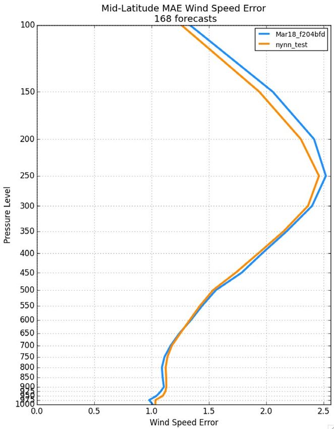
Example of Dynamic Spectral Mass-Flux Scheme
 HRRR 18-hour forecast
 Valid times: 12 UTC 24 June – 03 UTC 25 June 2020

 Negative = dry Positive = condensing
 10
Example Comparison of SW-up at Top of Atmosphere
 21 UTC 24 June 2020 Forecast hour 12, Initialized 09 UTC 24 June 2020

 Mass Flux
 GOES-16
 Satellite

Both Stratus + ShCu Edge
Mass-Flux PBLH
Components
active Surface
 A ShCu Edge B
 A
 B
 m s-1
 Dry portion of plumes Moist portion of plumes
Recent Development Activities:
 Removing Numerical
Pathologies in the MYNN-EDMF
Stress Test:
Hurricane SCM case
• No diurnal cycle
• Over land
• 60 m s-1 wind speeds
• Moderate/Low background moisture
• Clouds develop after hour 4

Configuration:
• Dx=2 km, dt=15 sec
• MYNN-EDMF
• MYNN surface layer scheme
Stress Test:
 Hurricane SCM case

• TKE-based PBLH develops quickly and extends
 up to ~5 km
• MYNN SGS clouds do not initiate earlier, but
 thicken the clouds after hr 12
• SGS cloud mixing ratios tend to be similar to or
 slightly larger than the resolved-scale mixing
 ratios
The Problem: Noisy Eddy Viscosity Profiles
KM = qlmS M = SQRT(TKE)lmS M

 Mixing length

 Stability function
The Cause:
The Mellor-Yamada framework uses different stability functions for each
closure level, making use of prognostic variables at each level.
The use of two different forms of stability functions in growing (q2.5/qeq < 1)
and decaying (q2.5/qeq > 1) turbulence regimes, where q2.5 is the prognosed
TKE and qeq is level 2.0 “equilibrium” TKE.
Note: Even when running at level 2.5, the level 2.0 stability functions were
used in the growing turbulence regime.

Possible Fixes:
1) Use only the level 2.5 forms of SM and SH for all regimes.
2) Use only the level 2.0 forms of SM and SH for all regimes.
Using only the level 2.5 stability functions

Note: It was necessary to add additional constraints from Helfand and
Labraga (1988) to achieve a computationally stable version.
• This suggests that the original coding was intended as so.
• Consequence: when the limits are hit for either (or both) SM and SH, the Prandtl
 number (Pr = KM/KH = SM/SH) can be regulated by the limits.
Hr 18 (mostly equilibrated)
Regionally Averaged Temperature Error Profiles
Mid-Latitude Global MAE
MAE

 Control
 Updated MYNN

Mid-Latitude Global Bias
Bias
Zonal Temperature Diffs (against GFS analyses)
 Control Updated MYNN
Regionally Averaged Wind Error Profiles
Mid-Latitude Tropics MAE
MAE

 Control
 Updated MYNN

 Tropics Bias
Mid-Latitude
Bias
Zonal Mean Wind Speed Differences (against GFS Analysis)
 Control Updated MYNN
Results from a RRFS Retro (4 -11 Sept 2020):
 CONUS composite stats against radiosonde

 Wind Speed Bias (fcst hr 12) Wind Speed RMSE (fcst hr 12)

 Original
 Updated MYNN
 Difference
More Results from a RRFS Retro (4 -11 Sept 2020):
 CONUS composite stats against radiosonde

 Temperature Bias (fcst hr 12) Temperature RMSE (fcst hr 12)

 Original
 Updated MYNN
More Results from a RRFS Retro (4 -11 Sept 2020):
 CONUS composite stats against radiosonde

 RH(obT) Bias (fcst hr 12) RH(obT) RMSE (fcst hr 12)

 Original
 Updated MYNN
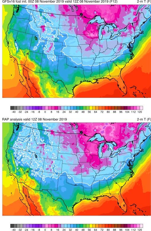
NATIONAL OCEANIC AND ATMOSPHERIC ADMINISTRATION

Radiational Cooling Case Performed by
 Alexei Belochitski

 Valid: 12Z 8 November 2020

 • Relaxed pressure gradient across
 much of Midwest, Plains, and
 western U.S., implying very light
 winds and likely overnight
 decoupling

 • 10m wind field (lower right) and
 cloud fields (not shown) indicate
 ideal conditions for radiation
 inversions and strong cooling over
 much of the U.S.

 • Visually comparing analysis (lower
 right) to GFSv16 (upper right)
 clearly shows it’s too warm over
 much of the Midwest, Northern
 Plains, and the Intermountain
 West
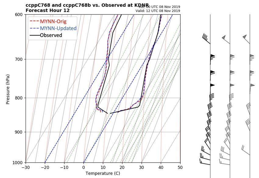
NATIONAL OCEANIC AND ATMOSPHERIC ADMINISTRATION

 GFSv16 Temperatures Performed by
 Alexei Belochitski

 Denver, CO DNR

 Init: 00Z 8 November 2019
 Valid: 12Z 8 November 2019 (F012)

 • GFSv16 failed to capture the
 strength of the low-level inversion
 and ends up way too warm at the
 lowest levels
 • GFS-MYNN improves the surface
Td bias = -8 C T bias = +6 C temperature and dewpoint, and is
 Td bias = -4 C T bias = +4 C
 warmer than GFS at the inversion
 top
Simulations performed by
 Alexei Belochitski

Very little/no impact
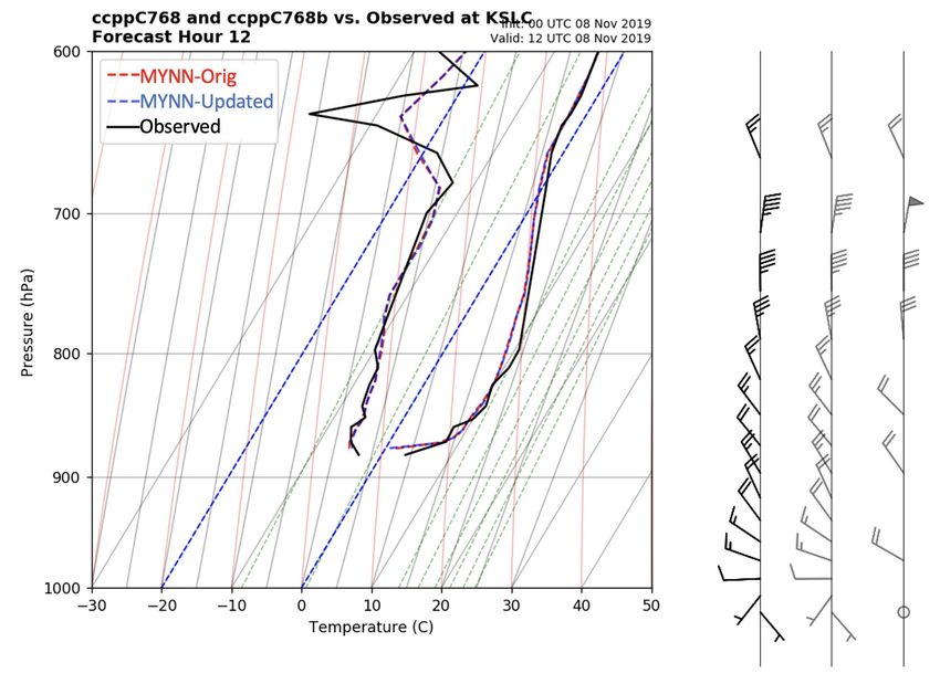
NATIONAL OCEANIC AND ATMOSPHERIC ADMINISTRATION

 SLC Soundings

 Salt Lake City, UT SLC

 Init: 00Z 8 November 2019
 Valid: 12Z 8 November 2019 (F012)

 • GFSv16 fails to capture the
 strength of the low-level inversion
 and ends up ~5 C too warm at the
 lowest levels
 • GFS-MYNN is colder and moister,
 but is slightly too cold at the
 surface.
Td bias = -3 C T bias = +5C
 Td bias = -2 C T bias = -2 C
Simulations performed by
 Alexei Belochitski

Very little/no impact
SCM SGP LLJ case
 m s-1
Setup:
 Jet max = 23 m s-1
• CCPP SCM
• Model top=100 mb
• 51 levels
• timestep: 60 sec

Results:
 Jet max = 19 m s-1
• Increased jet max
• Jet is still weaker and less sharp than in lidar
 observations
• Still investigating forcing/vertical resolution

 Jet max = 17 m s-1
Summary for Work on Numerical Pathologies
• Numerical pathology was diagnosed – stability functions were the cause
 o Switching to the level 2.5 stability functions provides some improvements
 o Concerned about hitting limits – impacting the Prandtl number (Pr = Sm/Sh)
 o Further investigation is required

• Impacts seem to improve the wind and temperature profiles
 o Largest improvements are in the upper troposphere
 o Concerned about a negative wind speed bias at low-levels

• Eddy-diffusivity-specific regime testing:
 o Updated stability functions do not adversely impact successful radiational cooling
 stable-layer cases
 o Low-level jet SCM case was improved
Improving Clouds
 GOES-R Observations

Comparison of SW-up at TOA
Valid: 16 UTC 12 June 2019
Initialized 06 UTC 11 June
 (Forecast hour 34)

 HRRR v4 HRRR v3
Despite improvements, there are still large biases
 Comparisons were made
 to GML’s 14 SurfRad/
 SolRad sites across the
 CONUS

 Aspects to revise/investigate:
 1) Cloud depth
 2) Cloud cover
 3) Mixing ratios (qc, qi, qs, etc)
 4) Liquid/Ice/Snow water path
 5) Hydrometeor effective radii
 6) Cloud overlap
 7) Diurnal cycle of shallow cumulus, etc…
Recent Development Activities:
 Higher-Order Moment
 Cloud PDF for Stratus Clouds
Chaboureau-Bechtold Stratiform Cloud Fraction:
 First-Order Form Higher-Order Form
The subgrid variability of the saturation deficit, s, is expressed The subgrid variability of the saturation deficit, s, is expressed
in terms of the total water, qw, and liquid water temperature: solely as the square root of the total water variance, q’2:
 1/2
 −1
 � 2 1/2
 = �2 − 2 � + � 2
 −2
 = 2
 ,

Where is a tuning constant, is the mixing length, and a
and b are thermodynamic functions arising from the And then the normalized saturation deficit is specified as:
linearization of the function for the water vapor saturation 1 = ( − ( � ))/ .
mixing ratio. Then, the same cloud fraction function is used as in the first-
 order form.
 −1
 ( )
 ( )
 � = 1 + � � = �

 + TOGA COARE
 o ARM
 � − ( � ))/
Normalized saturation deficit: 1 = (

Cloud fraction: = {0, [1, 0.5 + 0.36 (1.55 1 )]} cf
 cf = cf × m
 m = 1 + (MAX(RH- RHc, 0)/(RHss-RHc))1.9, where RH is the
 relative humidity, RHc = 0.75 and RHss = 1.01
 Taken from Chaboureau and Becthold (2002, JAS) 37
Introducing a Level 2.6 configuration • Prognoses TKE and q´2 (instead of just TKE) • Currently, q´2 is not advected • Makes the increased computational cost very small • Introduce a new bl_mynn_closure namelist variable: 2.5, _ _ ≤ 2.5 (TKE) Closure = � 2.6, 2.5 < _ _ < 3.0 (TKE and q´2) 3.0, 3.0 ≤ _ _ ∀∀∀∀ (TKE, q´2 , ´q´, and ´2) • Note: the higher-order (q´2) cloud PDF can be used with any closure level, but will use the diagnostic form of q´2 when bl_mynn_closure = 2.5
Impact on Diagnosed Cloud Water at 500 m
 1st-Order σs q´2 - σs
Impact on Diagnosed Cloud Ice at 300 mb
 1st-Order σs q´2 - σs
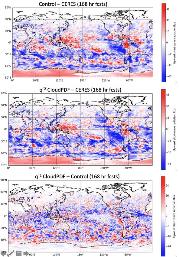
Upward SW Radiation at TOA
20 Oct – 29 Dec, Init every 5 days, Averaging day 6 fcsts
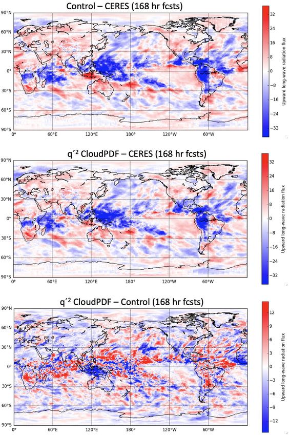
Upward LW Radiation at TOA
20 Oct – 29 Dec, Init every 5 days, Averaging day 6 fcsts
Improvements from
 Single-Column Modeling
SCM work in WRF and CCPP has shown:
o Good performance for LASSO shallow cumulus Publications:
 cases Angevine et al. 2018, Shallow Cumulus in
o Improved tuning of mass flux component WRF Parameterizations Evaluated against
 LASSO Large-Eddy Simulations. Monthly
o Need for more careful consideration of scale- Weather Review, vol. 146, pp. 4303-4322.
 aware features
 Angevine et al. 2020, Scale Awareness,
o Improved understanding of how to specify forcing Resolved Circulations, and Practical Limits
 and interpret SCM results in the MYNN–EDMF Boundary Layer and
o Using many cases avoids over-fitting Shallow Cumulus Scheme. Monthly
 Weather Review, vol. 148, pp. 4629-4639.
o Easy testing of different vertical grids
o Built capacity and collaboration among GSL and
 CSL groups
Accelerating Plume Modification
 The only distinguishing aspect to each plume is the entrainment rate
 i, which is taken from Tian and Kuang (2016):

 =

 Where li is the plume diameter, and C = 0.33.

 For large plume sizes, this form can produce a positive feedback
 between large wi and i, causing shallow cumulus to become too
 deep.

 This modification increases the entrainment in accelerating plumes
 above the cloud base.

 Hereafter, this is will be referred to as the ACP mod.

Adapted from Neggers (2015, JAMES)
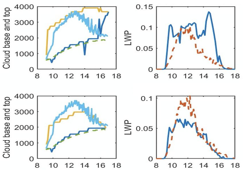
Example of improvement with the ACP mod
 LASSO 14 July 2019

CTL

ACP

 LES Cloud Top -LES -SCM
 SCM Cloud Top
 LES Cloud Base • Accelerating plume modification drastically improves LWP and
 SCM Cloud base cloud depth evolution (note different vertical axis scales)
 • Smoother profiles with ACP
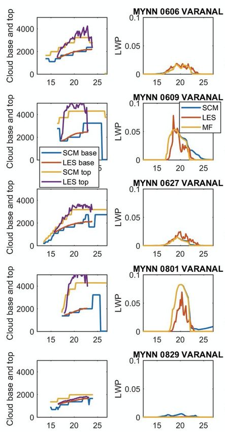
Testing the updated code in both
 WRF and CCPP

 Ten “good” LASSO cases from 2018 and 2019:

 • All SCM cases created from RAP analyses
 • WRF and CCPP results are fairly similar
 • Caveats: Vertical grids are not identical
 • Two cases have far too much cloud (0712
 and 1002)
 • Accelerating plume mod (“acp”) improves
 LWP and SWD (see later)
Nice, but we need to do better…

 RAP Dashed – Operational
 HRRR Solid – NextGen

Hour Hour
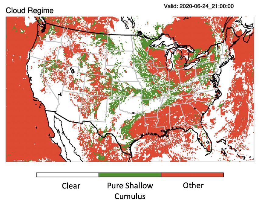
Ongoing/Future Work: Cloud Regime Diagnostic
 21 UTC 24 June 2020

GOES-16
Satellite

HRRR
 • Better characterize our errors in each regime
 • Link the errors to dominant processes in each regime
 • Refine the cloud macro- and microphysics in each regime, i.e.,
 cloud fraction, mixing ratios, effective radii, overlap, etc
Summary
• Development of the MYNN-EDMF has been equally focused on turbulence
 and cloud-radiative processes, exploiting both mass-flux and HOC.
• Testing in a hierarchy of models: global, regional, and SCM. Using LES as
 much as observations.
• Numerical pathologies associated with the stability functions have been
 alleviated
 • Overall improvements were found in bulk global and regional retrospective tests as
 well as 3D and SCM case studies
• Excessive cloudiness in the shallow-cumulus regime was caused by a
 positive feedback between the plume entrainment and vertical velocity
 • Modified entrainment in accelerating moist plumes addresses this problem
 • Improvements in LWP and SW-down were demonstrated
• Future work is planned to better sort the radiation errors by cloud regime
 and investigate the cloud-overlap in shallow-cumulus regimes
Extra slides
TKE Budget Fixes
Important fixes from Franciano Puhales:
• Vertical Transport term
• Vertical indexing
• Now accurate to within the level of noise.

RES = QWT + QSHEAR + QBUOY + QDISS
DTKE = TKEt – TKEt-1

 and

DIFF = RES – DTKE (well in the noise)
Example Comparison of SW-up at Top of Atmosphere
 21 UTC 24 June 2020 Forecast hour 12, Initialized 09 UTC 24 June 2020

GOES-16
Satellite No SGS Clouds – all
 clouds are from the
 Thompson
 microphysics scheme

Stratus
component Both Stratus +
only Mass-Flux components
Mapping the contribution of each plume
 to the total fractional area
The fraction grid area assumed to contain The number density, , of plume sizes is
coherent updrafts, au (%), is set to be represented by a power law:
proportional to the surface buoyancy flux (ℓ)=Cℓ
(Hsfc, W m-2): where C is a constant of proportionality, ℓ is the
 diameter of the plume, and d is the slope of the
 au = 10.0{0.5tanh[(Hsfc - 30)/90] + .5}, power-law relationship. effectively weights the
 contribution each plume size in au:
au varies between ~10% for Hsfc > 200 W m-2
and as small as 3-4% for Hsfc near 0 W m-2. Taken from Neggers et al. 2003, JAS

 Note:
 For d < -2, smaller
 LCL plumes dominate au
 For d > -2, larger
 plumes dominate au

 au
 The slope (d) is -1.9 ± 0.3 for the
 scales below the scale break.
 53
Chaboureau and Bechtold Subgrid Cloud Fraction:
Stratus & Convective components
Stratus Component Convective Component
The subgrid variability of the saturation deficit, s, is expressed The subgrid variability of the saturation deficit is proportional
in terms of the total water and liquid water temperature: to the mass-flux, M:
2 1/2
−1 ℎ
� −2 ℎ −
− = � 2 − 2 � + � 2 − ≈ ≈ ( / ∗ )
∗ ∗
Where is a tuning constant, is the mixing length, and a
and b are thermodynamic functions arising from the Where is a constant of proportionality (≈6E-3) and f is a
linearization of the function for the water vapor saturation vertical scaling function, set to f= � −1 .
mixing ratio.
2 2 + TOGA COARE
Combined saturation deficit variance − = − + − o ARM
−1
( ) ( )
� = � cf
� = 1 + �
Normalized saturation deficit � − ( � ))/ −
1 = (
Subgrid cloud fraction = {0, [1, 0.5 + 0.36 (1.55 1 )]}
Taken from Chaboureau and Becthold (2002, JAS)
cf+ = cf × m
m = 1 + (MAX(RH- RHc, 0)/(RHss-RHc))1.9, where RH is the relative humidity, RHc = 0.75 and RHss = 1.01 54You can also read