Black-Box Safety Validation of Autonomous Systems: A Multi-Fidelity Reinforcement Learning Approach
←
→
Page content transcription
If your browser does not render page correctly, please read the page content below
Black-Box Safety Validation of Autonomous Systems: A Multi-Fidelity
Reinforcement Learning Approach
Jared J. Beard1 and Ali Baheri2
Abstract— The increasing use of autonomous and semi-
autonomous agents in society has made it crucial to validate
their safety. However, the complex scenarios in which they are
used may make formal verification impossible. To address this
challenge, simulation-based safety validation is employed to test
arXiv:2203.03451v3 [eess.SY] 2 Mar 2023
the complex system. Recent approaches using reinforcement
learning are prone to excessive exploitation of known failures
and a lack of coverage in the space of failures. To address
this limitation, a type of Markov decision process called the
“knowledge MDP” has been defined. This approach takes into
account both the learned model and its metadata, such as
sample counts, in estimating the system’s knowledge through
the “knows what it knows” framework. A novel algorithm that Fig. 1: The MF-RL-falsify algorithm is applied to a grid
extends bidirectional learning to multiple fidelities of simulators world scenario where the aim is to train an adversary to
has been developed to solve the safety validation problem. The intercept a system under test, which is defined as failure
effectiveness of this approach is demonstrated through a case
study in which an adversary is trained to intercept a test model
in this study. The lowest fidelity having an unknown policy
in a grid-world environment. Monte Carlo trials compare the is selected and the corresponding simulator is sampled at
sample efficiency of the proposed algorithm to learning with a each time step. Information about learned models is used to
single-fidelity simulator and show the importance of incorporat- augment the reward structure, preventing early convergence
ing knowledge about learned models into the decision-making of the algorithm and ensuring continued exploration for
process.
failures.
I. INTRODUCTION
The process of safety validation checks if a system meets
with disturbances that result in system failure. AST has been
performance standards or identifies the nature of potential
applied in various real-world domains, from aircraft collision
failures. This is crucial in situations where human safety is
avoidance [6] to autonomous vehicles [7]. Despite its over-
at risk or significant harm to expensive equipment may occur,
all success, sampling-based methods such as reinforcement
such as in aircraft autopilots, driverless cars, and space-flight
learning have two main limitations. They may not be able to
systems. Formal verification, which is a commonly used
find rare failures [8], and they rely on data collected from
method, builds a detailed mathematical or computational
high-fidelity simulators, which may not be feasible due to
model of the system being tested to ensure it meets safety
computational constraints [9].
specifications. However, a major challenge in using formal
The requirement of relying solely on samples from high-
methods for safety validation is the large and complex design
fidelity simulators can be reduced by incorporating reinforce-
space of decision-making models, which makes it difficult for
ment learning techniques that utilize multiple levels of sim-
formal verification techniques to work effectively.
ulator fidelity [10]. The degree of accuracy of a simulator is
Another way of performing safety validation is through
referred to as its fidelity, with the level of fidelity representing
black-box and grey-box safety verification, where the system
how much the system model and assumptions are simplified.
is either not known well enough or only provides limited
Low-fidelity simulators make strong assumptions, leading
information for analysis, respectively [1]. These methods can
to faster execution, but may not exhibit realistic behavior
include planning algorithms [2], [3], optimization tools [4],
and dynamics. On the other hand, high-fidelity simulators
[5], and reinforcement learning [6]. From a reinforcement
aim to closely approximate reality, but their execution may
learning viewpoint, the goal of adaptive stress testing (AST)
be slower due to more complex system models and fewer
is to determine the most probable failure scenarios by treating
assumptions.
the problem as a Markov decision process (MDP) and finding
Related work. To date, there has been only one study on
an adversarial policy that associates environmental states
multi-fidelity (MF) safety validation, as described in [11].
1 Jared J. Beard is a Ruby Distinguished Doctoral Fellow with the This work serves as the only existing MF alternative to our
Mechanical and Aerospace Engineering Department at West Virginia Uni- proposed approach, where information is only passed from
versity, Morgantown, WV 26505, USA. jbeard6@mix.wvu.edu low to high-fidelity simulators in a unidirectional manner.
2 Ali Baheri is with the Mechanical Engineering Department at
Rochester Institute of Technology, Rochester, NY 14623, USA. However, unidirectional techniques limit the amount of in-
akbeme@rit.edu formation that can be passed, which affects their efficiency.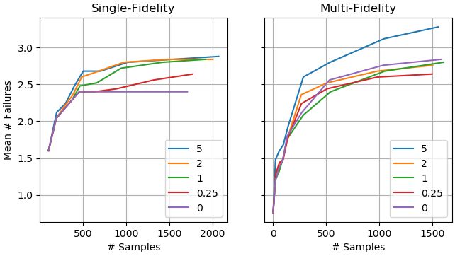
On the other hand, bidirectional approaches like the one to a failure metric. The work presented here seeks to reduce
presented in this paper, which pass information in both the need for computationally expensive simulations by using
directions, have been found to have lower sample complexity. MF simulations with bidirectional information passing to
The upper bound of high-fidelity samples in bidirectional improve the overall sample efficiency.
approaches is equivalent to the unidirectional case [10].
A. Markov Decision Process
Although this bidirectional approach is not used for safety
validation, it provides valuable insights into the problem. This work relies on MDP’s so it is useful to introduce
The bidirectional approach in this paper uses the “knows notation which will form the foundation of this work. MDP’s
what it knows” (KWIK) framework to evaluate the relative are defined by the tuple hS, A, T, R, γi. Here, S is the set
worth of a sample in a given fidelity. The KWIK framework of all states s and A the set of all actions a. The stochastic
is a concept in reinforcement learning (RL) that involves transition model is T (s0 | s, a), where s0 represents a state
explicitly tracking the uncertainty and reliability of learned outcome when taking a from s. R(s, a, s0 ) is the reward for
models in the decision-making process. The RL algorithm in some transition. Lastly, γ is a temporal discount factor. By
the KWIK framework is equipped with metadata about the solving an MDP, an optimal control policy π ∗ (s) ∀s ∈ S can
learned models, such as sample counts, and uses this infor- be achieved. Here, the optimal policy is defined as follows:
mation to estimate the system’s knowledge. This knowledge π ∗ (s) = arg max Q(s, a), (1)
is then used to guide the exploration-exploitation trade-off a
in the RL algorithm. where Q∗ (s, a) the corresponding optimal state-action value
Statement of contributions. The objective of this work is function is
to develop a framework that minimizes the simulation cost
while maximizing the number of failure scenarios discov- Q∗ (s, a) =
ered. In contrast to previous safety validation techniques, X
max T (s0 | s, a)[R(s, a, s0 ) + γQ∗ (s0 , a0 )]. (2)
we propose a learner that uses knowledge about itself to
s0
reformulate the safety validation problem and present a bidi-
rectional algorithm MF-RL-falsify to solve this problem B. Knows What It Knows Learner
(Fig. 1). The contributions of this work are as follows: Use of MF simulators in reinforcement learning has come
• We propose a novel knowledge Markov decision process about from the desire to reduce the number of samples in
(KMDP) framework, which factors knowledge (i.e., and expense incurred by high-fidelity simulators used to get
metadata) of the learned model into the decision making reliable performance. To this end, [10] leveraged the concept
process and explicitly distinguishes the system model of KWIK learners [12]. The fundamental idea of KWIK is
from the knowledge of this model; to use information about the learned model to provide output
• We demonstrate MF-RL-falsify an algorithm using indicating its confidence in said model. When the learner is
the KWIK framework to train learners from multi- not confident in the model, it reports relevant state-action
ple fidelities of simulators in a bidirectional manner. pairs as unknown (⊥) [12]. In particular, Cutler, et al. uses
MF-RL-falsify also uses a knowledge-based update the number of samples to assert a model is known to some
to prevent early convergence of the learned model and degree of confidence specified by the Hoeffding inequality
encourage further exploration. (parameterized by , δ) [10].
Paper structure. The paper is structured as follows: Section In the multi-fidelity case, the knowledge is used to decide
II briefly outlines preliminaries, as well as introduces the when to switch between the D fidelities of simulators. The
KMDP. Section III details the MF-RL-falsify algorithm. knowledge K is defined for this work as both estimates
Section IV covers the experimental setup, results, and some of the transition and reward models (K.T̂ , K.R̂), as well
limitations of the implementation. Lastly, Section V presents as the confidence in these models Kd,T (s, a), Kd,R (s, a) .
concluding remarks and future directions of work. Here, the subscript d indicates the specific fidelity. The lower
fidelities aim to guide search in higher fidelity simulators,
II. P ROBLEM SETUP AND P RELIMINARY while knowledge from higher fidelities is used to improve
The objective of this work is to find the most likely failure the accuracy of lower fidelity models. Mathematically, two
scenarios for a (decision-making/control) system under test simulators are said to be in fidelity to each other if their Q
M. Here, failure scenarios are defined as the sequence of values are sufficiently close according to:
transitions that lead to some failure condition (e.g., midair
collision). The system under test is placed in a black-box f (Σi , Σj , ρi , βi ) =
(usually high-fidelity) simulator Σ, so the learner (with ∗ ∗
∆ = − maxs,a |Qi (s, a) − Qj (ρj (s), a)|,
planner P ) does not have direct access to the internal ∀s, a if ∆ ≤ βi (3)
workings of the system. The learner then samples scenarios
−∞, else.
iteratively to learn and uses the planner to apply disturbances
(e.g., control agents in the environment, supply noise, or Note, β indicates a user specified bound on how dissimilar
adjust parameters of the environment). More specifically, two simulators can be and ρ is a mapping of states from the
the learner uses the simulations to minimize the distance fidelity of i to fidelity j. In this work, this mapping is applied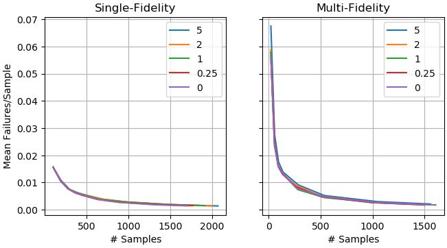
on a state-by-state basis, as the decision process only needs       evaluateState simulates trajectories and updates the learned
to model one decision at a time, not the whole system.              models. Lastly, marginalUpdate, given confidence informa-
                                                                    tion, updates the reward function to bias search away from
C. Knowledge Markov Decision Process                                trajectories for which the models are known (sampled a
   Whereas this learning problem has classically been rep-          sufficient number of times). The proposed algorithm is ini-
resented as an MDP, doing so assumes the model is known             tialized with a set of simulators, fidelity constants, and state
with sufficient accuracy. This may not always be the case           mappings hΣ, β, ρi, the system under test M, and the planner
(as in reinforcement learning). When the decision maker can         P of choice (this work uses value iteration). Additionally,
quantify its lack of information about the model, it should be      the confidence parameters (, δ), and minimum samples to
able to use this information to its benefit. Thus, we introduce     change fidelity (mknown , munknown ) are supplied. For more
the KMDP as hS, A, T, R, K, γi. Here, K represents the              information on the choice of these parameters, see [10]. With
knowledge about the decision maker’s model of the system            no samples, K is initialized with a uniform distribution over
(e.g., estimates of the other terms hS, A, T, Ri, confidence in     transitions and rewards set as Rmax of the KMDP. The Q
those estimates, and other assumptions of the learned model).       values are set to 0 and the current fidelity d is declared as
Consequently, T̂ and R̂ are used to solve the underlying MDP        the lowest fidelity. Lastly, it is assumed there are no changes
as the agent learns. Note from Sec. II-B these estimates of         to the model estimate, and no known or unknown samples
the model are considered part of K. In doing so, the learner        (mk , mu ).
is explicitly aware that it is making decisions based on an
estimated model of its environment and that it has some             A. Search
domain knowledge regarding the quality of these estimates.
                                                                       The search algorithm serves primarily to initiate the
Thus this information can factor into decisions, such as
                                                                    learning process. MF-RL-falsify looks at failures from
through the reward which is now defined as R̂(s, a, s0 , K).
                                                                    a single initial condition. As such, a state s is passed in
As an example, knowledge about the lack of information
                                                                    along with a desired number of trajectories n. The estimate
for some subset of states could necessitate a reward that
                                                                    of the set of failure modes, F̂ is initialized as empty. For
encourages exploration in those regions.
                                                                    every iteration, the simulators are reset and evaluateState
   The KMDP is related to the concepts of maximum like-
                                                                    is called. Failure scenarios found by evaluateState are
lihood model MDPs and reward shaping. The maximum
                                                                    added to F̂. Due to the nature of sampling, policies may
likelihood model MDP and KMDP share similar update rules
                                                                    come from more than one fidelity. Thus, after the search
for the learned reward and transition models [13]. However,
                                                                    has concluded, it is necessary to evaluate whether failure
KMDP generalizes these concepts to include estimates of
                                                                    modes are viable in the highest fidelity; those not meeting
S and A, as well as providing a more broad use of the
                                                                    this condition are rejected. The remaining set is returned to
information gained from sampling. As an example, the agent
                                                                    the user. Plausibility checks may manifest in a few ways:
may not be aware of all states if it is required to explore
                                                                    for simulators with relatively simple transition models, these
its environment, thus the estimated state space would be
                                                                    can be checked directly to exist or not; for more complex,
a subset of S. Furthermore knowledge may now capture
                                                                    stochastic systems, this may involve a Monte Carlo sampling
concepts such as whether a state has been visited, which
                                                                    to determine if a transition occurs in the model. Fortunately,
is not inherently captured by the underlying state. It is
                                                                    due to the Markov assumption, this can be broken down to
important to note that this would break the Markov property,
                                                                    a state-by-state basis, as opposed to looking at the entire
but such an approximation has been used to break explicit
                                                                    trajectory at once.
temporal dependencies [14]. The second concept is reward
shaping, where the additional reward terms guide learning as
                                                                    B. State Evaluation
a function of the system state [15]. The difference being that
here the learner is deciding based on learned information or           At every iteration of the search algorithm, the evaluat-
knowledge about the model, not only the underlying state.           eState function attempts to find a failure scenario given the
Following from this, Q∗ cannot actually be achieved, and the        current model estimate. The process begins by initializing
best Q given K becomes                                              the trajectory f . Then actions are iteratively selected from
                      X                                             the current policy π and the decision is made to increment
   QK (s, a) = max                                                  the fidelity or sample the current one. This continues until a
                   a
                       s0                                           terminal state is found; terminal states can be a failure event,
        K.T̂ (s | s, a)[K.R̂(s, a, s0 , K) + γQK (s0 , a0 )]. (4)
               0
                                                                    exceeding the maximum number of time steps, or reaching
                                                                    some state where failure cannot occur. Whenever the fidelity
III. FALSIFICATION USING MULTI - FIDELITY SIMULATORS                is incremented, both mk and mu are reset. Otherwise, if
   Here, the functionality of the MF-RL-falsify algo-               a known state-action is reached, mk is incremented, while
rithm (Alg. 1) is described. The approach centers on three          mu is reset. The converse occurs when an unknown state
functionalities: search, evaluateState, and marginalUpdate.         is reached. Similarly, changed is set to false when the state
The search function is tasked with iterating through tri-           is incremented and set to true when a state-action becomes
als and collecting failure information. As part of search,          known.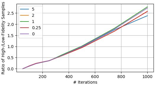
The fidelity is decremented if a known state has not
Algorithm 1: MF-RL-falsify                           recently been reached and the lower fidelity states are also
 input: hΣ, β, ρi, M, Rinc , P , (, δ),             unknown. This permits more efficient search by using the
  (mknown , munknown )                               less expensive simulator to carry out uncertain actions. Along
 initialize: K, Qd                                   with the decrement, the planner is updated using the current
 initialize: changed = f alse, d = 1, mk , mu = 0    model. Otherwise, a simulation is performed to gather data
 Procedure search(s,n)                               from the model. If the current state is considered unknown,
     F̂ ← {}                                         this information is used to update the learned model and
     for i = 1, ..., n do                            knowledge. The knowledge about the transition is incre-
          reinitialize(Σ)                            mented by one (the distribution is generated by normalizing
          F̂ ← F̂ ∪ evaluateState(s)                 the sampled outcomes for each s, a pair). The reward is
                                                     updated as a weighted average of the reward estimate and
     for f ∈ F̂ do
                                                     sampled reward. Lastly, the knowledge about each, being the
         if ¬isP lausible(f, D) then
                                                     number of samples for a state-action, is incremented by one.
             F̂ ← F̂ \ f
                                                     If a state-action becomes known, the planner is updated. The
    return F̂                                        transition is added to the trajectory and the current state is
 Procedure evaluateState(s)                          updated. Subsequently, the fidelity is incremented and re-
    initialize: f ← {}                               planning occurs if enough known samples have been visited.
    while ¬terminal(s) do                            The algorithm concludes with the marginal update if the
        a ← {P.π(s), M.π(s)}                         trajectory has converged all (s, a) ∈ f considered known .
        if d > 1 and changed and                     If a failure state has been achieved by the trajectory, the
          Kd−1 (ρd−1 (s), aP ) =⊥ and                trajectory is deemed a failure scenario and returned.
          mu ≥ munknown then                            When planning, the algorithm must pass information to
             Qd−1 ← plan(d − 1)                      lower fidelities to improve the performance of future sam-
             d←d−1                                   ples. The plan function does this by finding the highest
        else                                         fidelity (≥ d) for which a state-action pair is known. This
             s0 , r ∼ TΣ (s0 | s, a)                 model estimate is then used to update the knowledge of the
             if Kd (s, a) = ⊥ then                  current fidelity. Similarly, to pass information up, if states
                   update Kd (s, a)                  from the current d and next lower d − 1 model estimates are
                   if Kd (s, a) 6= ⊥ then            deemed to be in fidelity (∆ ≤ β), the lower fidelity model
                       Qd ← plan(d)                  estimate is used in place of the current fidelity. The planner
             f ← f ∪ hs, a, s0 i, s ← s0             is then run to update Q.
         if d < D and mk ≥ mknown then
             Qd+1 ← plan(d + 1)                      C. Marginal Update
             d←d+1
                                                        The marginal update incorporates knowledge into the
     if isConverged(f ) then                         decision making process. Here, the marginal is defined as the
          marginalU pdate(f )
                                                     difference in the best state-action value QK and the second
     if isF ailure(f ) then                          best state-action value QK0 for a given state. When the
          return f                                   system is known to be converged, the state having the largest
 Procedure plan(d)                                   marginal (along the trajectory) is selected. Using this state,
    for all hs, ai do                                the reward is decreased by Rinc and the planner updated.
       d0 ← {max(d0 ) | d0 ≥ d, Kd0 (s, a) 6=⊥}      The underlying idea is that if the learner has converged on a
       Kd (s, a) ← Kd0 (s, a)                        trajectory, it will cease to explore the solution space, exploit-
                                                     ing an action repeatedly. By finding the state where the best
    return P.train(K.T̂ , K.R̂, Qd , Qd−1 + βd−1 )
                                                     action is significantly greater than its neighbors, exploration
 Procedure marginalUpdate(f )                        can erode the most functionally important actions for a given
    mmax ← 0, t ← hi                                 trajectory. As training continues, this cuts off search in more
    for hs, a, s0 i ∈ f do                           fragile trajectories (hence less likely trajectories early) and
        m = QK (s, a) − QK0 (s, a0 )
                                                     encourages exploration along the entirety of more robust
        if m > mmax then
            mmax ← m                                 failure trajectories.
            t ← hs, a, s0 i
     R(t) ← R(t) − Rinc                                                      IV. RESULTS
     Qd ← plan(d)
                                                       We evaluate the effectiveness of the proposed algorithm
                                                     by answering the following research questions:
• RQ1: Does the proposed multi-fidelity algorithm im-
prove the overall sample efficiency?1
• RQ2: Does the proposed multi-fidelity algorithm result
in the identification of more failure scenarios compared
to the single-fidelity scenario?
Before presenting the simulation setup, we define two key
terms in our experiments.
Definition 1. (Fidelity). In this context fidelity refers to the
accuracy of the model being used, with a high-fidelity model
having a higher level of accuracy, capturing more details
Fig. 2: 4×4 Grid worlds under test (left) low-fidelity, (right)
and nuances, while a low-fidelity model may not capture
high-fidelity. Here, fidelity is demonstrated by accuracy of
all the relevant information and result in less accuracy. In
the model, where the low-fidelity does not capture the impact
our experiments, the low-fidelity model does not accurately
of puddles on the transition model. The blue dot indicates
capture the impact of puddles on the transition model (see
the system under test, the red the MF-RL learner, and the
Fig. 2).
green “×” the system under test’s goal. Puddles are indicated
Definition 2. (Failure). Here, failure is defined as the scenario
by black and grey regions.
where the red dot (MF-RL learner) intersects the blue dot
(system under test).
A. Simulation
The experiment involved a 4×4 grid world environment
with puddles (as depicted in Fig. 2). The goal of the system
under test was to reach a specific location in the grid world,
while the learner’s objective was to cause failures by either
blocking the system under test or causing a collision. The
system under test was designed to be myopic, meaning it
would take the closest unobstructed action towards its goal.
The states were defined by the coordinates of both the system
under test (x, y)M and the learner (x, y)P . Both agents were
able to move one cell in any of the cardinal directions or
remain in place. If an agent was in a puddle, it had a 20% Fig. 3: Mean ratio of high-fidelity samples to low-fidelity
chance of reaching the desired cell; otherwise, it would not samples against iterations of search; notice that Rinc = 5
move. The learner was penalized based on its distance from encourages more exploration as samples increase. Legend
the system under test, receiving a penalty of −5 when in indicates values of Rinc .
a puddle and −25 when the system under test reached the
goal. If the learner induced a failure, it received a reward of
50. The discount factor γ was set to 0.95 for the experiment. likely far below this convergence estimate. For context, the
optimal high-fidelity policy could be found at a high- to
B. Monte Carlo Trials
low-fidelity sample ratio of less than ∼ 0.4. Notice that the
To evaluate the approach, 25 Monte Carlo trials were con- marginal update does not appreciably impact the ratio, except
ducted for both the single-fidelity (SF) and MF learners. To for Rinc = 5, where the search reached under-explored
evaluate the performance of the marginal update, each of five states in low fidelities. Naturally, as the algorithm converges,
values for Rinc = [0, 0.25, 1, 2, 5] at up to 1000 iterations return to lower fidelities is prevented and the samples grow
were used in both simulators. Note that Rinc = 0 indicates at approximately the same rate as the SF case, hence the
no marginal update. Each trial, the initial coordinates of near linear behavior after convergence (Fig. 4) (RQ1). In
the system under test and learner were uniformly sampled; the SF scenario, increasing Rinc led to further search, though
samples that obviously could not cause failures or scenarios in the MF scenario the behavior was unclear, likely due to
initialized to failure states were removed. Other parameters interactions from changing fidelities.
were set as follows: β = 1250, tmax = 20, = 0.25, With respect to the number of failures, the MF simula-
δ = 0.5, mknown = 10, and munknown = 5. tor quickly accumulates failures from low-fidelity samples,
Given the relatively simple scenario, it is helpful to while the earliest high-fidelity samples in the SF simulator
understand where the MF simulator converges in the highest are wasted (Fig. 5) (RQ2). Around convergence, their perfor-
fidelity. Much larger examples involve sparse scenarios, so mance is comparable. Without the marginal update, search
the area of interest are those regions where the ratio of high- in SF ceases at convergence; a large Rinc yields ∼ 15%
fidelity to low-fidelity samples (Fig. 3) is relatively low and increase in failures found. In the MF scenario, small updates
1 Sample efficiency refers to the ability of the RL agent to learn effectively perform similarly to no update, however, Rinc = 5 yields a
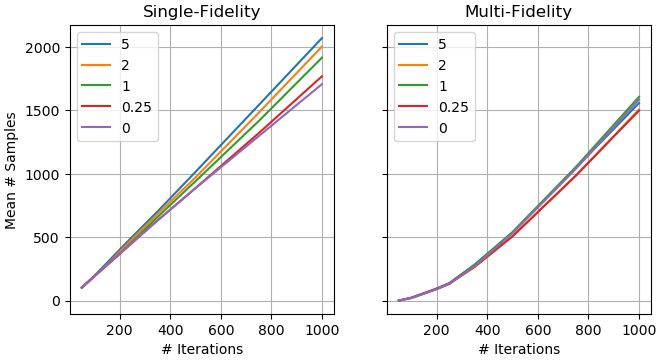
from a relatively small number of environment interactions. significant improvement, as much as 15% with almost noFig. 4: Mean number of high-fidelity samples for (left) Fig. 6: Ratio of failures per sample for the (left) single-
single-fidelity and (right) Multi-fidelity learners. Notice the and (right) multi-fidelity cases. The MF approach is approx-
MF approach accumulates significantly fewer samples until imately 6 times more efficient for few samples; their effi-
convergence, at which samples are accumulated at similar ciency converges as samples increases. Additionally Rinc =
rates. Legend indicates values of Rinc . 5 appears to provide an upper bound on the performance.
Legend indicates values of Rinc .
be challenging within the KWIK framework. The second
limitation is that value iteration, which is used to find
solutions to MDPs, is not very efficient and thus limits the
number of Monte Carlo trials and the size of the environment.
This issue could potentially be resolved by using an anytime
solver such as Monte Carlo tree search [16].
V. CONCLUSIONS
The purpose of this study was to enhance the effectiveness
of reinforcement learning techniques in detecting failure
Fig. 5: Mean number of high-fidelity failures for the (left)
scenarios in autonomous systems. The study introduced the
single- and (right) multi-fidelity approaches. The MF ap-
knowledge MDP, which incorporates a learner’s understand-
proach immediately makes use of underlying information,
ing of its own model estimates into the decision-making pro-
while the SF approach wastes early samples in the high-
cess, through the KWIK framework. The resulting algorithm,
fidelity simulator. Additionally, Rinc = 5 increases the
called MF-RL-falsify showed improved performance
number of failures found relative to no or a small update.
compared to single-fidelity (SF) approaches. The inclusion
Legend indicates values of Rinc .
of knowledge through marginal updates was also found to
increase exploration in converged scenarios and enhance
early exploration of the solution space.
HF samples, supporting use of the marginal update. The
However, further development is needed for the technique
improvements of the MF scenario are further realized in Fig.
to become a viable alternative to existing methods. This
6. The MF scenario finds as many as 6 times more failures
includes increasing scalability by utilizing learned models
per sample than the SF case early on, with their performance
with anytime planners and applying the framework to contin-
approaching unity after convergence.
uous state and action spaces. Additionally, further research is
Overall, results are promising, indicating the MF algorithm necessary to test the KMDP formulation in various contexts
significantly improves the sample efficiency in finding failure and more complex scenarios.
scenarios over the SF approach. Additionally, the marginal
update for large values of Rinc enhances exploration con- R EFERENCES
sistently with growth in samples, leading to more failure
scenarios and greater sample efficiency, particularly when [1] A. Corso, R. Moss, M. Koren, R. Lee, and M. Kochenderfer, “A
survey of algorithms for black-box safety validation of cyber-physical
the model has been sampled insufficiently (as in more systems,” Journal of Artificial Intelligence Research, vol. 72, pp. 377–
complicated scenarios). 428, 2021.
[2] E. Plaku, L. E. Kavraki, and M. Y. Vardi, “Hybrid systems: from
verification to falsification by combining motion planning and discrete
C. Limitations search,” Formal Methods in System Design, vol. 34, no. 2, pp. 157–
The implementation has two main drawbacks. One is 182, 2009.
[3] C. E. Tuncali and G. Fainekos, “Rapidly-exploring random trees for
that it is only created for discrete problems and handling testing automated vehicles,” in 2019 IEEE Intelligent Transportation
representations of knowledge and continuous domains can Systems Conference (ITSC). IEEE, 2019, pp. 661–666.[4] G. E. Mullins, P. G. Stankiewicz, R. C. Hawthorne, and S. K. [14] J. J. Beard, Environment Search Planning Subject to High Robot
Gupta, “Adaptive generation of challenging scenarios for testing and Localization Uncertainty. West Virginia University, 2020.
evaluation of autonomous vehicles,” Journal of Systems and Software, [15] A. D. Laud, Theory and application of reward shaping in reinforce-
vol. 137, pp. 197–215, 2018. ment learning. University of Illinois at Urbana-Champaign, 2004.
[5] J. Deshmukh, M. Horvat, X. Jin, R. Majumdar, and V. S. Prabhu, [16] C. B. Browne, E. Powley, D. Whitehouse, S. M. Lucas, P. I. Cowling,
“Testing cyber-physical systems through Bayesian optimization,” ACM P. Rohlfshagen, S. Tavener, D. Perez, S. Samothrakis, and S. Colton,
Transactions on Embedded Computing Systems (TECS), vol. 16, “A survey of Monte Carlo tree search methods,” IEEE Transactions on
no. 5s, pp. 1–18, 2017. Computational Intelligence and AI in games, vol. 4, no. 1, pp. 1–43,
[6] R. Lee, O. J. Mengshoel, A. Saksena, R. W. Gardner, D. Genin, 2012.
J. Silbermann, M. Owen, and M. J. Kochenderfer, “Adaptive stress
testing: Finding likely failure events with reinforcement learning,”
Journal of Artificial Intelligence Research, vol. 69, pp. 1165–1201,
2020.
[7] M. Koren, S. Alsaif, R. Lee, and M. J. Kochenderfer, “Adaptive stress
testing for autonomous vehicles,” in 2018 IEEE Intelligent Vehicles
Symposium (IV). IEEE, 2018, pp. 1–7.
[8] A. Corso, R. Lee, and M. J. Kochenderfer, “Scalable autonomous
vehicle safety validation through dynamic programming and scene
decomposition,” in 2020 IEEE 23rd International Conference on
Intelligent Transportation Systems (ITSC). IEEE, 2020, pp. 1–6.
[9] R. J. Moss, R. Lee, N. Visser, J. Hochwarth, J. G. Lopez, and M. J.
Kochenderfer, “Adaptive stress testing of trajectory predictions in
flight management systems,” in 2020 AIAA/IEEE 39th Digital Avionics
Systems Conference (DASC). IEEE, 2020, pp. 1–10.
[10] M. Cutler, T. J. Walsh, and J. P. How, “Real-world reinforcement
learning via multifidelity simulators,” IEEE Transactions on Robotics,
vol. 31, no. 3, pp. 655–671, 2015.
[11] M. Koren, A. Nassar, and M. J. Kochenderfer, “Finding failures in
high-fidelity simulation using adaptive stress testing and the backward
algorithm,” in 2021 IEEE/RSJ International Conference on Intelligent
Robots and Systems (IROS). IEEE, 2021, pp. 5944–5949.
[12] L. Li, M. L. Littman, T. J. Walsh, and A. L. Strehl, “Knows what
it knows: A framework for self-aware learning,” Machine learning,
vol. 82, no. 3, pp. 399–443, 2011.
[13] M. Wiering and J. urgen Schmidhuber, “Learning exploration policies
with models,” Proc. CONALD, 1998.VI. APPENDIX Algorithm 2: KWIK
The KWIK formulation (Alg. 2) was generated by strip- input: Σ, M, Rinc , P , (, δ)
ping MF-RL-falsify of its dependence on fidelity. As initialize: K, Q
such, supplying MF-RL-falsify with a SF simulator, will Procedure search(s,n)
have the same performance. In spite of this, the KWIK F̂ ← {}
algorithm was used for experiments. Notice, there is no for i = 1, ..., n do
longer a need to check the veracity of failures since all reinitialize(Σ)
samples are from a single fidelity. Furthermore, planning is F̂ ← F̂ ∪ evaluateState(s)
accomplished using the models for T̂ and R̂ as there is no return F̂
longer information to pass. This reduces the plan step to Procedure evaluateState(s)
training as would be done in classical approaches. initialize: f ← {}
while ¬terminal(s) do
a ← {P.π(s), M.π(s)}
s0 , r ∼ TΣ (s0 | s, a)
if K(s, a) = ⊥ then
update K(s, a)
if K(s, a) 6= ⊥ then
Q ← P.train(K.T̂ , K.R̂, Q)
f ← f ∪ hs, a, s0 i, s ← s0
if isConverged(f ) then
marginalU pdate(f )
if isF ailure(f ) then
return f
Procedure marginalUpdate(f )
mmax ← 0, t ← hi
for hs, a, s0 i ∈ f do
m = QK (s, a) − QK0 (s, a0 )
if m > mmax then
mmax ← m
t ← hs, a, s0 i
R(t) ← R(t) − Rinc
Q ← P.train(K.T̂ , K.R̂, Q)You can also read