Biotic interactions are an unexpected yet critical control on the complexity of an abiotically driven polar ecosystem
←
→
Page content transcription
If your browser does not render page correctly, please read the page content below
Biotic interactions are an unexpected yet critical control on the
complexity of an abiotically driven polar ecosystem
Lee, C. K., Laughlin, D. C., Bottos, E. M., Caruso, T., Joy, K., Barrett, J. E., Brabyn, L., Nielsen, U. N., Adams, B.
J., Wall, D. H., Hopkins, D. W., Pointing, S. B., McDonald, I. R., Cowan, D. A., Banks, J. C., Stichbury, G. A.,
Jones, I., Zawar-Reza, P., Katurji, M., ... Cary, S. C. (2019). Biotic interactions are an unexpected yet critical
control on the complexity of an abiotically driven polar ecosystem. Communications Biology, (2), [62].
https://doi.org/10.1038/s42003-018-0274-5
Published in:
Communications Biology

Document Version:
Publisher's PDF, also known as Version of record

Queen's University Belfast - Research Portal:
Link to publication record in Queen's University Belfast Research Portal

Publisher rights
© 2019 The Authors.
This article is licensed under a Creative Commons
Attribution 4.0 International License, which permits use, sharing,
adaptation, distribution and reproduction in any medium or format, as long as you give
appropriate credit to the original author(s) and the source, provide a link to the Creative
Commons license, and indicate if changes were made. The images or other third party
material in this article are included in the article’s Creative Commons license, unless
indicated otherwise in a credit line to the material. If material is not included in the
article’s Creative Commons license and your intended use is not permitted by statutory
regulation or exceeds the permitted use, you will need to obtain permission directly from
the copyright holder. To view a copy of this license, visit http://creativecommons.org/
licenses/by/4.0/.
General rights
Copyright for the publications made accessible via the Queen's University Belfast Research Portal is retained by the author(s) and / or other
copyright owners and it is a condition of accessing these publications that users recognise and abide by the legal requirements associated
with these rights.

Take down policy
The Research Portal is Queen's institutional repository that provides access to Queen's research output. Every effort has been made to
ensure that content in the Research Portal does not infringe any person's rights, or applicable UK laws. If you discover content in the
Research Portal that you believe breaches copyright or violates any law, please contact openaccess@qub.ac.uk.

Download date:24. Dec. 2020
ARTICLE
                  https://doi.org/10.1038/s42003-018-0274-5                 OPEN

                  Biotic interactions are an unexpected yet critical
                  control on the complexity of an abiotically driven
                  polar ecosystem
1234567890():,;

                  Charles K. Lee         et al.#

                  Abiotic and biotic factors control ecosystem biodiversity, but their relative contributions
                  remain unclear. The ultraoligotrophic ecosystem of the Antarctic Dry Valleys, a simple yet
                  highly heterogeneous ecosystem, is a natural laboratory well-suited for resolving the abiotic
                  and biotic controls of community structure. We undertook a multidisciplinary investigation to
                  capture ecologically relevant biotic and abiotic attributes of more than 500 sites in the Dry
                  Valleys, encompassing observed landscape heterogeneities across more than 200 km2. Using
                  richness of autotrophic and heterotrophic taxa as a proxy for functional complexity, we linked
                  measured variables in a parsimonious yet comprehensive structural equation model that
                  explained significant variations in biological complexity and identified landscape-scale and
                  fine-scale abiotic factors as the primary drivers of diversity. However, the inclusion of lin-
                  kages among functional groups was essential for constructing the best-fitting model. Our
                  findings support the notion that biotic interactions make crucial contributions even in an
                  extremely simple ecosystem.

                  Correspondence and requests for materials should be addressed to S.C.C. (email: craig.cary@waikato.ac.nz).
                  #
                    A full list of authors and their affiliations appears at the end of the paper.

                  COMMUNICATIONS BIOLOGY | (2019)2:62 | https://doi.org/10.1038/s42003-018-0274-5 | www.nature.com/commsbio    1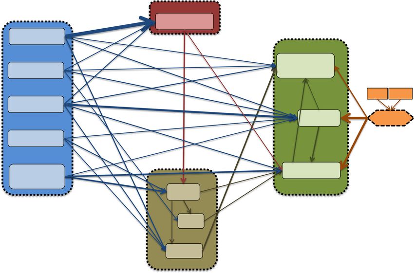
ARTICLE                                                               COMMUNICATIONS BIOLOGY | https://doi.org/10.1038/s42003-018-0274-5

U
         nderstanding how ecosystems self-organize at landscape             soils20,21,24–27. The extreme environmental conditions and lack of
         scales has long been a formidable challenge in ecology1,2          evidence for critical biotic interactions have made ecologists
         since the trophic complexity of most ecosystems obscures           hypothesize that these ecosystems are fundamentally constrained
the relative contributions of the biotic and abiotic factors reg-           by abiotic factors and host some of the simplest trophic structures
ulating biological diversity3–6. Given the fundamental effects of           on Earth21,23,24,28,29 (Supplementary Figure 1). These unique
biodiversity on ecosystem function7, a critical task is to resolve          characteristics make the Dry Valleys a model system for resolving
the relative importance of three sets of ecological factors that            the roles of abiotic and biotic factors that shape community
drive community structure: abiotic environmental filtering, dis-             structure.
persal limitation in space, and biotic interactions (e.g., competi-            In this study, we analyzed data collected by the New Zealand
tion, mutualism, and trophic relationships)2,8. Thorough and                Terrestrial Antarctic Biocomplexity Survey (nzTABS, https://
spatially explicit descriptions of these ecosystem drivers are              ictar.aq/nztabs-science/), which was initiated during the Inter-
required for this task, but the complexity of most ecosystems               national Polar Year 2007–2008. This project draws on a wide
creates enormous logistical obstacles.                                      range of international expertise to profile the biology, geochem-
   Biotic interactions, including those among higher eukaryotes             istry, geology, and climate of the Dry Valleys, and has completed
and those between higher eukaryotes and microorganisms, have                a spatially and biologically comprehensive landscape-scale survey
long been recognized as important drivers of ecosystem structure            that aims to resolve the biotic and abiotic control of ecosystem
and function6,9. However, attempts to capture biotic interactions           complexity. We then used structural equation modelling (SEM)
at the ecosystem level have often been restricted both by sampling          to analyze the comprehensive collection of geological, geo-
approaches and/or the expertise of individual investigators10, and          graphical, geochemical, hydrological, and biological variables
studies have largely focused on testing hypotheses associated with          measured systematically across three Dry Valleys of Antarctica.
pre-identified biotic interactions or ecosystem components6,11–15.              Structural equation modelling (SEM), which is built on path
A comprehensive investigation of abiotic and biotic interactions            analysis and factor analysis, is one of the most useful statistical
within an ecosystem therefore requires a sampling design that is            approaches to disentangle numerous factors of influence30 and
consistent across all major biological groups present. It also              develop deeper causal understanding from observational data31.
requires an explicitly interdisciplinary and comprehensive                  Users of SEM translate theoretical frameworks (informed by
approach for data collection and analysis of both abiotic and               knowledge of the ecosystem) into explicit multivariate hypoth-
biotic variables.                                                           eses, and the SEM is used to evaluate whether the theory is
   For microorganisms (bacteria, archaea, and unicellular fungi),           consistent with empirical data30,32. A robust SEM allows
culture-independent characterization using molecular genetic                researchers to quantitatively assess the relative importance of
techniques is widely recognized as the most consistent and sen-             ecological drivers32,33 and is thus well suited for predicting eco-
sitive approach16, whereas conventional surveys remain the most             system responses to global change1,33.
reliable and practical approach for larger invertebrates and higher            In addition to challenging climatic conditions and hyperar-
animals and plants in terrestrial environments. For abiotic vari-           idity21, biotic interactions in Dry Valley soils are thought to be
ables and some major macroecological features (e.g., primary                limited by very low biomass and patchy distribution of photo-
productivity), geographic information system (GIS) has become               trophic communities28. Temperature and biologically available
an essential tool for collecting information across spatial scales.         water have been proposed as the primary determinants of species
The integration of GIS and remote sensing technologies (e.g.,               occurrence21,34, but the lack of studies explicitly addressing biotic
satellites) can provide spatially explicit environmental informa-           interactions in the Dry Valley ecosystems means that the role of
tion for entire geographic regions17,18. Specifically, the availability      biotic interactions is largely unknown (if present at all)28.
of high-resolution data layers from sources such as the Landsat 7           Therefore, our primary hypothesis was that abiotic environmental
and MODIS satellites facilitates complete and consistent                    filters are the major control on the biodiversity of this envir-
descriptions of environmental conditions (e.g., surface tempera-            onmentally extreme and simple terrestrial ecosystem, and the
ture and snow coverage) at the landscape scale18,19. Using these            structure of our SEM mostly reflected this notion. However, we
descriptions in conjunction with information on bedrock geology             found that linkages between different groups of biota and the
and geomorphology, it is now feasible to carry out systematic               groups’ discrete spatial patterns (i.e., independent of the effects of
landscape-scale surveys that capture heterogeneities in abiotic             spatial variation in abiotic factors) had to be included to obtain
conditions within an ecosystem. Additionally, all information               the best-fitting SEM. Overall, these findings indicate that biotic
collected within a GIS-enabled sampling framework is spatially              interactions make crucial contributions even in an extremely
explicit and enables thorough examinations of dispersal limita-             simple ecosystem.
tion effects across multiple spatial scales.
   Despite the advances in methodologies, disentangling the
relative roles of abiotic and biotic controls on the complexity in          Results
terrestrial ecosystems is still a major challenge in ecology. We            Correlations and nestedness of measured variables. Our data
propose that extreme ecosystems offer a natural laboratory to               indicated that richness (see Methods for definitions) was related
reduce this complexity while representing its major features20.             to community composition in each of the three groups of
Here, we offer an analysis of the controls on the biological                organisms examined (i.e., multicellular taxa, cyanobacteria, and
complexity of a region of the McMurdo Dry Valleys of Antarc-                fungi), which was to be expected given the low species richness of
tica. Located between the Polar Plateau and the Ross Sea (Fig. 1),          each group in the analyzed system. Multicellular taxon commu-
the McMurdo Dry Valleys (hereinafter the Dry Valleys) are the               nities were significantly nested (nestedness temperature = 17.56,
largest contiguous ice-free area on the Antarctic continent and             P = 0.010), and the richness of multicellular taxa was strongly
subject to some of the most extreme conditions of any terrestrial           correlated (r = −0.99, P = 0.001) with the first NMS axis of
habitat on Earth21, which severely constrain the range of biota             multicellular community composition. Nematodes were by far the
present22,23. Vascular plants and vertebrates are entirely absent,          most frequently observed organism, occurring in 80% of the
and soils are predominantly ultraoligotrophic, hyperarid, and               sampled tiles, followed by hypoliths (40%), rotifers (32%), lichens
often hypersaline21,22. Consequently, abiotic factors are widely            (25%), tardigrades (23%), springtails (19%), cyanobacterial mats
regarded as the primary force shaping the ecology of Dry Valley             (15%), mites (12%), and mosses (11%). Cyanobacterial

2                          COMMUNICATIONS BIOLOGY | (2019)2:62 | https://doi.org/10.1038/s42003-018-0274-5 | www.nature.com/commsbio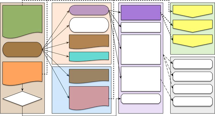
COMMUNICATIONS BIOLOGY | https://doi.org/10.1038/s42003-018-0274-5 ARTICLE
140.0 E 160.0 E 180.0 165.0 E
a b
Tasmania New Zealand Ross Sea 77.0 S
120.0 E
McMurdo
Dry Valleys
Indian Ocean Ross Island
Pacific Ocean
50.0 S
Ross Ice Shelf
Southern
Ross Sea Victoria Land 78.0 S
East Antarctica
70.0 S
c d
Garwood
valley
Shangri-La
Marshall
valley
Miers valley
0 2.5 5
km
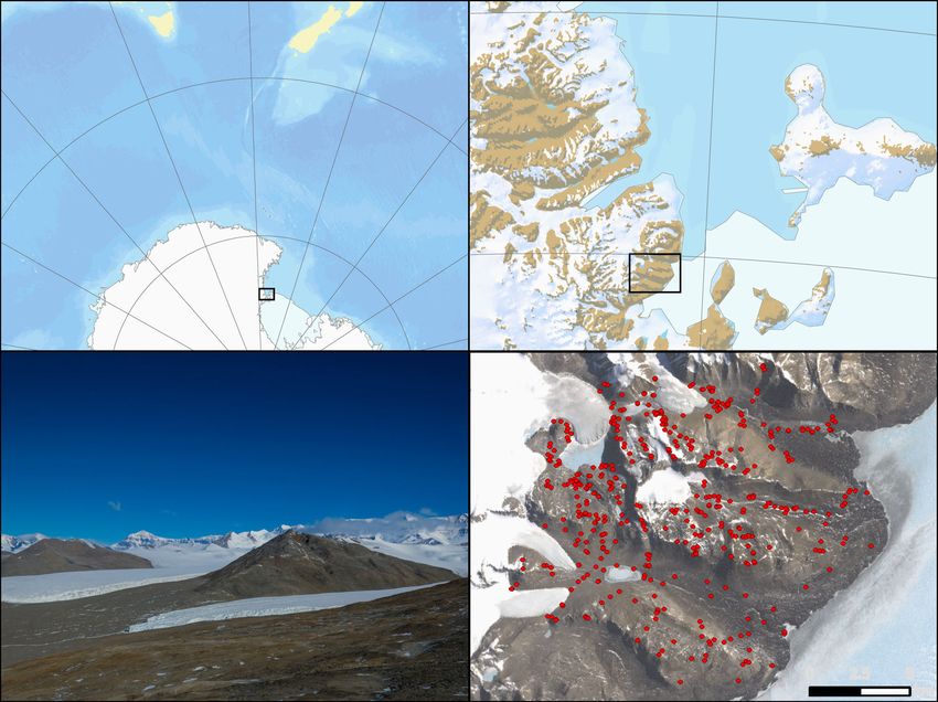
Fig. 1 Maps. a Southern Victoria Land (denoted by black rectangle) relative to East Antarctica and New Zealand (Image Credit: the World Topographic
Map, ArcGIS Online, Esri); b the McMurdo Dry Valleys (nzTABS study area denoted by black rectangle) relative to southern Victoria Land; c westward
view of the Miers Valley toward the Royal Society Range; and d the nzTABS study area, including Miers, Marshall, and Garwood Valleys (sampling sites
denoted by red dots) (Image Credit: the Landsat Image Mosaic of Antarctica [LIMA] Project)
communities were significantly nested (nestedness temperature (the standardized path coefficients can be interpreted as partial
= 2.01, P = 0.010), and cyanobacterial richness was correlated correlation coefficients). The model explains between 30 and 40%
with both NMS axes (axis 1: r = −0.75, axis 2: r = −0.66, P = of the variance in the richness variables (i.e., Multicellular Taxa S,
0.001) derived from the cyanobacterial community matrix. Fun- Cyano S, and Fungal S), which are strongly correlated with
gal communities were also significantly nested (nestedness tem- community composition, as described above. Importantly, soil
perature = 2.61, P = 0.010), and fungal richness was correlated properties do not clearly mediate the effects of topography and
with both NMS axes (axis 1: r = 0.61, axis 2: r = −0.79, P = climate on biotic diversity, and topographic and climate variables
0.003) derived from the fungal community matrix. have many important direct pathways to biota. Attempts to trim
the model by removing select pathways substantially reduced the
Structural equation models. The initial a priori SEM (Supple- goodness-of-fit of the model, so each pathway is important. This
mentary Figure 2) did not fit the data well (Comparative Fit Index model is particularly valuable and robust because it explicitly
[CFI] = 0.706, χ2 = 394.397, df = 43, P < 0.0001). This initial accounts for spatial patterns that do not depend on environmental
model only included pathways that were well supported by pre- variables (see Methods). For example, some areas could be richer
vious empirical studies at the time the model was fit. This initial in species simply because they are located in regions that receive a
result made it clear that our a priori expectations were missing higher supply of immigrants supporting local populations even
important relationships within the ecosystem that were not well when conditions are not favorable. The ‘total effects’ (i.e., sums of
known in the literature. Consequently, to obtain a model with an direct and indirect effects) of each environmental variable on each
implied covariance structure that matched the observed data well, biotic variable (Multicellular Taxa S, Cyano S, and Fungal S)
we made two modifications. First, we identified missing pathways indicate that elevation, slope, aspect, distance to coast, and wetness
that contributed to poor model-fit by inspecting the residual index all have significant total effects on richness and composition
covariance matrix and added as few of these theoretically plausible of multicellular taxon and microbial assemblages (Supplementary
pathways as possible (e.g., direct pathways from abiotic variables Table 1).
to biotic variables). Second, we removed non-significant pathways.
The final model (Fig. 2a) fits the data well (CFI = 0.996, χ2 = Importance of biotic interactions. It is also important to note
45.018, df = 35, P = 0.1196) and represents the most parsimo- that the positive links among the richness of multicellular taxon
nious model possible. Each pathway in the model is significant and microbial assemblages were essential to the model;
COMMUNICATIONS BIOLOGY | (2019)2:62 | https://doi.org/10.1038/s42003-018-0274-5 | www.nature.com/commsbio 3ARTICLE COMMUNICATIONS BIOLOGY | https://doi.org/10.1038/s42003-018-0274-5
a
R 2 = 0.42 Microclimate
–0.60 Temperature
Elevation –0.10
–0.14
R 2 = 0.33
0.12
–0.09 Multicellular
Aspect taxa S
0.16
–0.21
0.25
0.16 0.11 s1 s2
0.15
Dist. to coast
–0.13 –0.40
0.33 Cyano S Space
–0.11
–0.08 R 2 = 0.36
Slope 0.09
0.20 –0.34
–0.15
0.16
–0.22
0.12 0.24
Wetness Fungal S
index R 2 = 0.13
0.25 0.16 R 2 = 0.40
Water –0.10
0.15 0.17
Topography –0.09 –0.16 Biodiversity
pH
0.12
R2 = 0.04
Soil N
R 2 = 0.08
Soil properties
b c d
High High High
Cyanobacteria Low Fungi Low Multicellular taxa Low
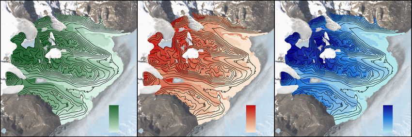
Fig. 2 Final structural equation model and predicted richness for three biotic groups. a Final structural equation model (CFI = 0.996, df = 35, χ2 = 45.018,
P = 0.1196) with standardized path coefficients (all paths significant, see the Mplus code in Supplementary Data 4). “S” represents the richness (and
composition) of multicellular taxon and microbial assemblages. “Space” represents environmentally independent spatial variables. Cyanobacterial richness
was positively correlated with elevation, distance to the coast, and the wetness index; negatively correlated with aspect (degrees from north) and slope;
and strongly related to spatial covariates. Fungal richness was positively correlated with distance from the coast, soil water content, and cyanobacteria
richness; negatively correlated with pH and temperature; and strongly related to spatial covariates. Richness of multicellular taxa was positively correlated
with cyanobacterial richness, fungal richness, soil nitrogen, distance to the coast, and elevation; negatively correlated with aspect; and less strongly related
to spatial covariates. Higher surface temperatures were associated with lower soil water content; and b–d predictions of cyanobacterial, fungal, and
multicellular taxon richness, respectively, across the landscape
removing these pathways yielded very poor model-fit indices. cyanobacterial richness to fungal richness and from cyano-
The chosen directions of these pathways were guided by both bacterial richness to multicellular taxon richness, given the
empirical data and theory. There were eight possible combi- foundational contribution of these autotrophic single-celled
nations of directed paths among three variables, and after organisms to this extreme ecosystem. Importantly, the positive
arriving at the final model (Fig. 2a), we tested all eight com- covariance among the biota is not simply due to similar
binations to evaluate the sensitivity to the directions of these responses to abiotic conditions because each group responds
pathways. Four of these eight models yielded poor-fitting individually to the sets of abiotic variables in the model
models (P < 0.05, specific models not shown), and each of these (Fig. 2a). This implies that processes other than abiotic filtering
poor models included a pathway from multicellular taxa to drive the positive covariance among the three groups of biota.
fungi, which is strong evidence against that particular pathway.
However, the other four models were indistinguishable from a Relative contributions of abiotic and biotic factors. Overall,
model-fitting perspective (all P > 0.05, specific models not environmental filtering imposed the strongest net effects on biotic
shown), and so we relied on theory to specify the direction of richness (Table 1). Spatial processes were the second most
these pathways. Ecological theory supports pathways from important set of richness drivers, with nearly the same magnitude
4 COMMUNICATIONS BIOLOGY | (2019)2:62 | https://doi.org/10.1038/s42003-018-0274-5 | www.nature.com/commsbioCOMMUNICATIONS BIOLOGY | https://doi.org/10.1038/s42003-018-0274-5 ARTICLE
of effect as environmental filtering for cyanobacteria (Table 1). Table 1 Net effects of various parameters on biological
Biotic interactions were important in determining fungal and richness
multicellular taxon richness, and their impact on multicellular
taxa was comparable to that of spatial processes (Table 1). Finally,
Abiotic Spatial Biotic
the SEM was used to generate spatially explicit predictions of
biodiversity across the study area (Fig. 2b–d) to demonstrate its Cyanobacteria 0.45 0.40 0
Fungi 0.42 0.34 0.20
potential as a tool for understanding the spatial heterogeneity of Multicellular Taxa 0.39 0.21 0.21
soil biota in the Dry Valleys for both scientific investigation and
environmental management. Net effects of abiotic environmental filters, spatial processes, and biotic interactions on
cyanobacterial, fungal, and multicellular taxon richness. Effects were calculated using composite
variables within the SEM and represent the absolute standardized path coefficients (ranging
from 0 to 1).
Discussion
Earlier investigators had suggested that the species richness of
Antarctic terrestrial vegetation south of 72°S35 and the structure model explicitly allowed each group to respond to a unique
of Dry Valley invertebrate communities26,36 are determined by combination of abiotic variables. Conversely, the set of correla-
local conditions. Our data and model show the prominence of tions that link the species richness of the three groups are
abiotic drivers (in particular total soil N, soil wetness index, essential to the fit of the model; removing them from the model
elevation, and distance to the coast) and support the general view produces models that fit the data very poorly.
that abiotic factors are the most important ecological filter in The Dry Valleys are arguably the simplest large-scale (4500
extreme environments2,20. However, there is a notable and large km2 of ice-free area39) ecosystem on the Earth. Therefore, a
amount of variance in the species richness of major functional small increase in the richness of any of the three major groups
groups and their reciprocal correlations that is not accounted for in this system may imply a disproportionate increase in the
by abiotic factors. Notably, soil ATP level (a proxy for biomass) biotic complexity of the system because every added species can
was not significantly correlated with any of the other variables bring in a new set of interactions between the three functional
measured and removed from the final model (Fig. 2a). In the groups. This is consistent with the trophic theory of island
absence of other practical measures of biotic variables, we believe biogeography, which is particularly relevant to systems such as
that species richness (which is significantly correlated with the Dry Valleys because they experience dispersal limitation
composition, see Methods) effectively captures biotic variables and disconnection between local communities37,40–43. Specifi-
within this study. cally, trophic constraints (i.e., species need their resource to
Our model shows that the spatial autocorrelation vectors (i.e., establish successfully) alter immigration and extinction
independent of variation in abiotic factors) are the second dynamics, which ultimately determine species richness. In the
strongest correlate of richness (Table 1). The spatial patterns Dry Valleys, food webs are particularly isolated compared to
accounted for by these autocorrelation vectors can be caused by other soil food webs, which should reduce the recruitment of
both unmeasured biological processes (e.g., dispersal limitation) lower trophic level species for their consumers. The low con-
and legacy effects (e.g., historic distribution of glaciers and pro- nectivity of the food webs in the Dry Valleys is thus expected to
glacial lakes)20. It is very unlikely that these spatial patterns are translate into lower immigration and higher extinction rates.
caused by major unmeasured environmental variables, given the This is expected to create high spatial and temporal variability
quantity and quality of the environmental measurements col- in species composition and richness, and contributes to food
lected in this study. It is possible that an unmeasured soil attri- webs dominated by generalist primary consumers with very few
bute (e.g., soil bulk density, water-holding capacity) could secondary consumers40,41. Overall, the patterns of species
account for some of the patterns observed. However, given the richness we observed are consistent with these dynamics and
variety of biotic variables captured in this study, it is unlikely that suggest that the diversity of the primary producers plays a
any single unmeasured abiotic variable will show strong corre- central role in driving the diversity of the other organisms. A
lation with measured biotic influences. Legacy effects are further implication is that understanding the drivers of
important in establishing and maintaining ice-free refugia for microbial diversity will be central to predicting higher trophic
terrestrial biota20,37, and the importance of the spatial vectors in level responses to environmental change, which is happening at
the SEM thus potentially supports a role for legacies linked to marked rates in polar regions44.
glacial geomorphology in shaping distributions of biota in the The empirical SEM (Fig. 2a) incorporated all measured factors,
Dry Valleys36,38. including soil physicochemical properties that cannot be obtained
Our model also shows that, besides spatial vectors and abiotic through remote sensing. Therefore, an additional SEM was
factors, a notable amount of variance in the species richness of derived using only unstandardized coefficients associated with
each group is explained by correlations between biotic groups. As factors that are obtainable through remote sensing and GIS (e.g.,
we further explain below, we hypothesize that these correlations wetness index, temperature, elevation, aspect, distance to the
reflect variation in the biological complexity of the ecosystem. coast, and slope) (Supplementary Figure 3). In the future, this
Specifically, our model highlights some of the major linkages in “predictive” SEM can be used to make spatially explicit predic-
the Dry Valleys ecosystem: in this system, cyanobacteria provide tions of biodiversity across the entire Dry Valley landscape.
the energetic foundation of food webs, and their species richness Ultimately, the model and its future version can be used to
does not appear to be influenced by the richness of fungi and support the development of best management practices for this
multicellular taxa (Table 1). However, fungal richness was highest unique ecosystem protected by the Antarctic Treaty System
where cyanobacterial richness was high, and multicellular taxon (http://www.ats.aq).
richness was highest where both cyanobacterial and fungal rich- In conclusion, we found that abiotic factors such as soil tem-
ness was high (Fig. 2b–d), highlighting the fundamental impor- perature and topography had important direct effects on richness
tance of autotrophic cyanobacteria as the primary producers in as well as indirect effects mediated through physicochemical soil
this extreme ecosystem. We are confident that the positive cov- properties (Fig. 2a). However, contrary to our expectations, we
ariance among the groups of organisms considered here is not also found that the correlations between the functional groups
confounded by covariation with abiotic conditions because the and spatial autocorrelation in the variation of the richness of the
COMMUNICATIONS BIOLOGY | (2019)2:62 | https://doi.org/10.1038/s42003-018-0274-5 | www.nature.com/commsbio 5ARTICLE COMMUNICATIONS BIOLOGY | https://doi.org/10.1038/s42003-018-0274-5
functional groups are a major determinant of the biological Table 2 Landscape-scale variables captured by nzTABS
diversity of the system. This result suggests that biotic factors are
an underestimated control on the complexity of the Dry Valley
Category Variables
ecosystem and raises the question of whether biotic interactions
and processes have been similarly underappreciated in other Remote Sensing and GIS (Satellite Elevationa
and LIDAR) Slopea
simple and/or extreme ecosystems. Furthermore, our findings Aspecta
highlight the fundamental importance of incorporating biotic Snow/Ice/Water Presencea
factors and spatial constraints when forecasting community Distance to the Coast
responses to changing environmental conditions. This has direct Soil Surface Temperature
relevance to more complex ecosystems where biotic interactions Wetness Index60
play a markedly greater role in shaping community structure and Geology Bedrock Geologya53
ecosystem functioning. Glacial Geomorphologya
Biology Lichen and Moss (Abundance and
Size)
Methods Endolith and Hypolith (Abundance)
Study area. Approximately 0.4% of Antarctica is permanently ice-free, and the
main ice-free areas are the Antarctic Peninsula, the McMurdo Dry Valleys, and Cyanobacterial Mat (Abundance
various mountains and nunataks along the Transantarctic Mountains21. Of these, and Size)
the McMurdo Dry Valleys contain the largest contiguously ice-free areas (~4500 - Invertebrates (Abundance and
km2) and have been the focus of terrestrial biology research on the continent for the Taxonomy)
past 50 years21,39. The McMurdo Dry Valleys are situated in southern Victoria Land ATP Level
along the western coast of McMurdo Sound (between 160–164°E and 76–78°S) and Bacterial Richness (ARISA)
contain markedly complex surface geology and topography that result in highly Cyanobacterial Richness (ARISA)
heterogeneous physicochemical conditions in soils across the landscape. The area Fungal Richness (ARISA)
chosen for this study comprises 220 km2 of largely ice-free terrain that includes
Garwood, Marshall, and Miers Valleys as well as Shangri-La, an area west of
Geochemistry pH
Marshall Valley and enclosed by Joyce Glacier, Mt. Pams, and Mt. Lama (Fig. 1). Conductivity
In addition to the extreme cold (mean annual air temperature of approximately Water Activity (Aw)
−20 °C), the McMurdo Dry Valleys are characterized by strong winds, extreme Total Soil Moisture Content
aridity (precipitation of 2 cm dia-
invertebrate taxon across much of the landscape, and their distribution and meter) removed aseptically and homogenized in a sterile 42 oz. Whirl-Pak; soil
abundance primarily correlate with the presence of liquid water, pH, salinity, and (~20 g) for moisture content measurement, subsampled from homogenized bulk
inorganic carbon45,46. Taxonomic diversity for nematodes is low (five species), but soil into a sterile 15 mL centrifuge tube sealed with Parafilm; soil (~300 g) for
abundances can be as high as hot desert soils23,46. Rotifers (four species) and microinvertebrate count, stored in a sterile 18 oz. Whirl-Pak (pebbles not
tardigrades (eight species) are present but more restricted to ephemerally wetted removed to minimize disturbance).
areas23,46. A single species of Collembola (Gomphiocephalus hodgsoni) represents A microarthropod survey (i.e., springtails and mites) was carried out by examining
the largest (albeit onlyCOMMUNICATIONS BIOLOGY | https://doi.org/10.1038/s42003-018-0274-5 ARTICLE
In-field
Genotyping
analyses Split for DNA Multicellular taxa S
extraction Bacteria
Vegetation and lithic & splits
community survey Cyanobacteria
Lichen Fungi
Moss Split for RNA
Endolith / hypolith extraction Genotyping Fungal S
Cyanobacterial mat (in lifeGuard) Archaea
Geochemistry Cyanobacterial S
pH/conductivity Community structure
Water activity 16S rRNA PCR amplicon
sequencing
Bulk soil samples (earth Microbiome project) Diversity indices
Biological activity (DOE JGI community
sequencing project)
ATP
Microbial biogeography
Macroinvertebrate survey
Additional geochemistry Community
Springtail
Total moisture content structure & function Interactions with abiotic
Mite environmental drivers
Total C & N Metagenomic sequencing
(DOE JGI community
sequencing project)
Ecosystem structure
Microinvertebrate survey
Diversity
Macroinvertebrate Abundance Population genetics
samples Live / dead Biogeography & evolution Ecosystem function
Age & gender
Lab
Tile sampling analyses Molecular analyses Additional analyses
Fig. 3 Flow diagram for nzTABS sample analysis. “S” represents the richness and composition of multicellular taxon and microbial assemblages. Solid lines
represent transfer or utilization of physical samples (including DNA), and dashed lines represent analysis of information. Colored components are included
in the present study
custom R and Python scripts, see Supplementary Data 2) that examines all peaks such as unintended duplicates and incorrect GPS location), data for 490 samples
between 100 and 1200 base pairs for cyanobacterial electropherograms and 100 were included in the analysis.
and 1400 base pairs for fungal electropherograms57. Peaks in these size ranges
that made up greater than 0.3% of all peaks over 30 relative fluorescence units in
each electropherogram were accepted as true peaks. The total number of true Data analysis. A broad suite of geological, geographical, geochemical, hydro-
peaks was taken as a measure of taxon richness for each sample. Peaks within logical, and biological variables (Table 2 and Supplementary Data 3) were collected
one base pair of one another were binned for the purpose of comparing and evaluated to derive the most parsimonious set of predictors of biodiversity in
electropherograms between samples. our study area. Biodiversity is represented by the richness of key autotrophic and
ARISA was used to measure richness due to its proven ability to detect and heterotrophic groups and the presence of known taxa. Specifically, species richness
discern diversity of edaphic cyanobacteria signals in the Dry Valleys over 16S of cyanobacteria and fungi was estimated using the number of ribosomal intergenic
rRNA gene PCR amplicons27,57 and its proven ability to capture fungal diversity spacer length-polymorphic fragments observed from community fingerprinting
patterns in Dry Valley soils in a consistent and cost-effective manner. analyses. These intergenic spacers exhibit length polymorphism across species and
even at the intra-species level, and the length profiles of PCR fragments are
therefore indicative of the diversity and abundance of microbial communities. We
note that these techniques do not resolve richness at a consistent taxonomic level;
Environmental metadata. A number of key environmental attributes were derived however, given that they can both over- and under-estimate species-level richness,
from satellite imagery and the DEM, including surface soil temperature, a topo- we do not believe the results were influenced by systematic biases. Taxon richness
graphically derived “wetness index”, and distance to the coast. Soil surface tem- for multicellular taxa was represented by the number of the following supraspecific
peratures were obtained from Landsat 7 ETM+ using band 6 (at 60 m resolution), taxa present in a sample: nematodes, rotifers, tardigrades, springtails, mites, cya-
which captured the up-welling thermal infrared spectrum (in the 10.4–12.5 μm nobacterial mats, mosses, lichens, and hypolithic consortia. These taxonomic
band). Landsat 7-derived temperature data corresponding to locations of forty-five groups also correspond to distinct trophic/functional groups in the system. Spe-
on-the-ground temperature loggers (DS1921G iButtons, Maxim Integrated, San cifically, the animals are all primary consumers of both bacteria and fungi, cya-
Jose, CA) were compared with records from the iButtons, and significant positive nobacteria are the main primary producers besides mosses, and fungi represent the
correlations between the two data sets were found59. major microbial decomposer group. Given the very low number of metazoan
Wetness index, which produces a relative index of liquid water availability in (Supplementary Figure 1), cyanobacterial57, and fungal49 species in the Dry Val-
summer, was calculated using a GIS-based model using variables that influence the leys, relatively small increase in the species richness of each compartment may
volume and distribution of water. Remote sensing images from the Moderate imply a marked increase in the complexity of the system in terms of increased
Resolution Imaging Spectroradiometer (MODIS) sensor collected over several number of ecological interactions.
years were used to calculate an average index of snow cover, which was then To verify that inferences made from patterns in species richness apply similarly
combined with other water sources such as glaciers and lakes. This resulted in a to community composition, richness was correlated with community composition
probable water source model representing the highly heterogeneous distribution of in all three groups of organisms (i.e., cyanobacteria, fungi, and multicellular taxa)
water sources in the Dry Valleys60. The water source model was used to weight a based on an analysis of nestedness (R script available upon request). Nestedness
hydrological flow accumulation model61 that used slope derived from LIDAR occurs when species-poor communities are generally subsets of species-rich
elevation data captured for most parts of the Dry Valleys50. These data were then communities, and when rare species tend to only occur in species-rich
used to calculate a Compound Topographic Index (CTI), a steady-state wetness communities. The nestedness of each of the three community matrices was
on both slope and upstream contributing area62. CTI takes the form:
index based evaluated by calculating their respective “temperatures”, which determine whether
As
CTI ¼ ln tan 2
β where As is the upslope contributing area in m per unit width species-poor communities are subsets of species-rich ones. The “temperatures”
orthogonal to the flow direction, and ß is the slope angle in radians63. The resultant were calculated using the “nestedtemp” function64 in the “vegan” library of R65,
model is a relative index of potential water availability, given the availability of melt and their significance was assessed via permutation using the “oecosimu” function.
water sources and topographical features. The relationship between richness and non-metric multidimensional scaling
Distance to the coast value was calculated as the Euclidean distance (in meters) (NMS) ordinations (based on Bray–Curtis similarity) of community composition
from the sampling point to the closest point on coastline, which in turn was (obtained using the “metaMDS” function in “vegan”)65 was quantified using
defined by cells with zero elevation in the DEM. Specifically, the shortest distance correlation analysis.
was determined by the perpendicular from the coastline to the sampling point. Overall, all these preliminary analyses supported the assumption that in the
After quality control (removal of tiles with missing or questionable information, specific system analyzed in this work, species richness of major functional groups is
COMMUNICATIONS BIOLOGY | (2019)2:62 | https://doi.org/10.1038/s42003-018-0274-5 | www.nature.com/commsbio 7ARTICLE COMMUNICATIONS BIOLOGY | https://doi.org/10.1038/s42003-018-0274-5
the best metric to describe the richness of each group as well as the correlations 2. Weiher, E. & Keddy, P. A. Assembly rules, null models, and trait dispersion:
between groups and the relationship between biota and abiotic factors. new questions from old patterns. Oikos 74, 159–164 (1995).
Cyanobacterial richness, rather than total bacterial richness, was included in our 3. Hanson, C. A., Fuhrman, J. A., Horner-Devine, M. C. & Martiny, J. B. H.
analysis for the following reasons. First, including both would effectively be Beyond biogeographic patterns: processes shaping the microbial landscape.
“double-counting” since total bacterial richness includes cyanobacteria as well. Nat. Rev. Microbiol. 10, 497–506 (2012).
Second, cyanobacteria are arguably the most critical group of bacteria, given their 4. Loreau, M. et al. Biodiversity and ecosystem functioning: current knowledge
large proportional input to primary production in this extreme environment. and future challenges. Science 294, 804–808 (2001).
Finally, cyanobacterial richness was significantly and positively correlated with
5. Lamb, E. G., Kennedy, N. & Siciliano, S. D. Effects of plant species richness
total bacterial richness (r = 0.31, P < 0.0001), so knowing the richness of one group
and evenness on soil microbial community diversity and function. Plant Soil
provides reasonable estimates about the richness of the other.
338, 483–495 (2010).
Biological communities closer in space are likely to be more similar in species
6. de Vries, F. T. et al. Abiotic drivers and plant traits explain landscape-scale
richness and community composition. However, historical population- and
landscape-level processes that are relatively independent of environmental conditions patterns in soil microbial communities. FEMS Microbiol. Ecol. 15, 1230–1239
can also be a driver of Antarctic biodiversity13,20,66,67. Thus, environmentally (2012).
independent spatial variables were computed to account for spatial patterns linked to 7. Cardinale, B. J. et al. Biodiversity loss and its impact on humanity. Nature 486,
intrinsic population- and landscape-level processes, such as dispersal limitation or 59–67 (2012).
source-sink dynamics8 (see Supplementary Methods). Competition- and predation- 8. Borcard, D. & Legendre, P. All-scale spatial analysis of ecological data by
related direct biotic interactions were not explicitly considered due to limited evidence means of principal coordinates of neighbour matrices. Ecol. Model 153, 51–68
for such interactions among Dry Valley biota23,28. (2002).
To represent spatial patterns driven by intrinsic population- and community- 9. van der Heijden, M. G. A., Bardgett, R. D. & van Straalen, N. M. The unseen
level processes (e.g., limited dispersal), environmentally independent spatial majority: soil microbes as drivers of plant diversity and productivity in
variables were obtained as follows. First, optimal (in terms of describing spatial terrestrial ecosystems. Ecol. Lett. 11, 296–310 (2008).
autocorrelation) combinations of Principal Coordinates of Neighbor Matrices 10. Bardgett, R. D. & Wardle, D. A. Aboveground-Belowground Linkages. (Oxford
(PCNM) were calculated8. To explicitly model spatial patterns that are independent University Press, Oxford, 2010).
of environmental gradients, the PCNMs were regressed against all environmental 11. Loreau, M. Linking biodiversity and ecosystems: towards a unifying ecological
variables to allow extraction of the residuals (aka “spatial residuals”). The “spatial theory. Philos. Trans. Roy. Soc. B 365, 49–60 (2010).
residuals” were then used in a linear regression model to predict the three biotic 12. Nielsen, U. N., Osler, G. H. R., Campbell, C. D., Burslem, D. F. R. P. & Van
richness variables, and their predicted values were derived. This was followed by a Der Wal, R. The influence of vegetation type, soil properties and precipitation
principal component analysis (PCA) on these predicted values, allowing spatial on the composition of soil mite and microbial communities at the landscape
patterns to be summarized in the multivariate distribution of the three biotic scale. J. Biogeogr. 37, 1317–1328 (2010).
richness variables. The first two components (“s1” and “s2”) accounted for 90% of 13. Caruso, T. et al. Stochastic and deterministic processes interact in the
the environmentally independent spatial patterns. Finally, the net effect of spatial assembly of desert microbial communities on a global scale. ISME J. 5,
variation (s1 + s2) was captured through the use of a composite variable (diamond 1406–1413 (2011).
shape)30. These two spatial vectors thus account for all the spatial variation that is 14. Bru, D. et al. Determinants of the distribution of nitrogen-cycling microbial
not explainable in terms of measured biotic and abiotic variables. This variation communities at the landscape scale. ISME J. 5, 532–542 (2011).
also implicitly account for the effects of spatial variation in unmeasured variables, 15. Zimmerman, N. B. & Vitousek, P. M. Fungal endophyte communities reflect
which contribute to autocorrelation in measured variables. environmental structuring across a Hawaiian landscape. Proc. Natl Acad. Sci.
Structural equation modelling (SEM) with composite latent variables was used to USA 109, 13022–13027 (2012).
determine the relative importance of abiotic conditions, biotic interactions, and spatial 16. Hugenholtz, P., Goebel, B. M. & Pace, N. R. Impact of culture-independent
patterns due to population- and community-level processes. Based upon previous studies on the emerging phylogenetic view of bacterial diversity. J. Bacteriol.
work known at the time the model was fit22,29,66–68, an a priori SEM of biodiversity 180, 4765–4774 (1998).
was built, in which topographic properties and surface temperature (summer average) 17. Boyd, D. S. & Foody, G. M. An overview of recent remote sensing and
are mediated through the effects of soil properties and indirectly influence the
GIS based research in ecological informatics. Ecol. Inform. 6, 25–36 (2011).
richness of cyanobacteria (which positively correlates with total bacterial richness as
18. Foody, G. M. GIS: biodiversity applications. Prog. Phys. Geog 32, 223–235 (2008).
described above), fungi, and multicellular taxa (Supplementary Figure 2). To identify
19. Bindschadler, R. et al. The Landsat image mosaic of Antarctica. Remote Sens
variables to be included in the a priori model, the entire set of predictors was
Environ. 112, 4214–4226 (2008).
evaluated to determine which variables were most likely to be important for reasons of
20. Convey, P. et al. The spatial structure of Antarctic biodiversity. Ecol. Monogr.
parsimony, thereby eliminating soil age, geology, soil C, and conductivity.
To derive a final model with good fit to the data from the a priori SEM, non- 84, 203–244 (2014).
significant pathways were removed, and theoretically justifiable pathways were 21. Cary, S. C., McDonald, I. R., Barrett, J. E. & Cowan, D. A. On the rocks: the
added that were deemed to be important through inspecting the residual microbiology of Antarctic Dry Valley soils. Nat. Rev. Microbiol. 8, 129–138
covariance matrices and modification indices. The relationship between biotic (2010).
richness and geology was analyzed using ANOVA, and the final SEM was found to 22. Wall, D. H. Global change tipping points: above- and below-ground biotic
explain more variation than geology alone. The “total effects” of each variable on interactions in a low diversity ecosystem. Philos. Trans. Roy. Soc. B 362,
each biotic variable were calculated (Supplementary Table 1), which provides an 2291–2306 (2007).
order to which factors are most important by taking into account both direct and 23. Adams, B. J. et al. Diversity and distribution of Victoria Land biota. Soil. Biol.
indirect effects (total effects = direct + indirect effects; indirect effects = sum of the Biochem. 38, 3003–3018 (2006).
products along each pathway). Finally, composite variables were used to estimate 24. Sokol, E. R., Herbold, C. W., Lee, C. K., Cary, S. C. & Barrett, J. E. Local and
the net effects of three constructs (abiotic environmental filters, spatial processes, regional influences over soil microbial metacommunities in the Transantarctic
and biotic interactions) on each of three biotic response variables (cyanobacterial, Mountains. Ecosphere 4, 136 (2013).
fungal, and multicellular taxon richness)30. 25. Pointing, S. B. et al. Highly specialized microbial diversity in hyper-arid polar
desert. Proc. Natl Acad. Sci. USA 106, 19964–19969 (2009).
26. Poage, M., Barrett, J. E., Virginia, R. A. & Wall, D. H. The influence of soil
Code availability. Python, R, and Mplus scripts used to analyze the data are
available in Supplementary Data 2 and 4. geochemistry on nematode distribution, McMurdo Dry Valleys, Antarctica.
Arct. Antarct. Alp. Res 40, 119–128 (2008).
27. Lee, C. K., Barbier, B. A., Bottos, E. M., McDonald, I. R. & Cary, S. C. The
Data availability Inter-Valley Soil Comparative Survey: the ecology of Dry Valley edaphic
The final environmental and biological datasets generated and analyzed during the microbial communities. ISME J. 6, 1046–1057 (2012).
current study are available as Supplementary Data 1 through 3. 28. Hogg, I. D. et al. Biotic interactions in Antarctic terrestrial ecosystems: are
they a factor? Soil. Biol. Biochem. 38, 3035–3040 (2006).
29. Barrett, J. E. et al. Terrestrial ecosystem processes of Victoria Land, Antarctica.
Received: 4 July 2018 Accepted: 3 December 2018 Soil. Biol. Biochem. 38, 3019–3034 (2006).
30. Grace, J. B. & Bollen, K. A. Representing general theoretical concepts in
structural equation models: the role of composite variables. Environ. Ecol. Stat.
15, 191–213 (2008).
31. Grace, J. B., Adler, P. B., Harpole, W. S., Borer, E. T. & Seabloom, E. W. Causal
networks clarify productivity-richness interrelations, bivariate plots do not.
References Funct. Ecol. 28, 787 (2014).
1. Eisenhauer, N., Bowker, M. A., Grace, J. B. & Powell, J. R. From patterns to 32. Grace, J. B. & Bollen, K. A. Interpreting the results from multiple regression
causal understanding: Structural equation modeling (SEM) in soil ecology. and structural equation models. Bull. Ecol. Soc. Am. 86, 283–295 (2005).
Pedobiologia 58, 65 (2015).
8 COMMUNICATIONS BIOLOGY | (2019)2:62 | https://doi.org/10.1038/s42003-018-0274-5 | www.nature.com/commsbioCOMMUNICATIONS BIOLOGY | https://doi.org/10.1038/s42003-018-0274-5 ARTICLE
33. Grace, J. B. et al. Guidelines for a graph-theoretic implementation of structural 61. Tarboton, D. G. A new method for the determination of flow directions and
equation modeling. Ecosphere 3, 73 (2012). upslope areas in grid digital elevation models. Water Resour. Res. 33, 309–319
34. Barrett, J. E. et al. Co-variation in soil biodiversity and biogeochemistry in (2010).
northern and southern Victoria Land, Antarctica. Antarct. Sci. 18, 535–548 62. Moore, I. D., Lewis, A. & Gallant, J. C. in Modelling Change in Environmental
(2006). Systems (eds. Jakeman, A. J., Beck, M. B. & McAleer, M. J.) 189–214 (John
35. Green, T. G. A., Sancho, L. G., Pintado, A. & Schroeter, B. Functional and Wiley and Sons Ltd, New York, 1993).
spatial pressures on terrestrial vegetation in Antarctica forced by global 63. Gessler, P. E., Moore, I. D., McKenzie, N. J. & Ryan, P. J. Soil-landscape
warming. Polar. Biol. 34, 1643–1656 (2011). modelling and spatial prediction of soil attributes. Int J. Geogr. Inf. Syst. 9,
36. Janetschek, H. in Antarctic Ecology (ed. Holdgate, M. W.) 871–885 (Academic 421–432 (1995).
Press, New York, 1970). 64. Rodríguez-Gironés, M. A. & Santamaría, L. A new algorithm to calculate the
37. McGaughran, A., Hogg, I. D. & Stevens, M. I. Patterns of population genetic nestedness temperature of presence-absence matrices. J. Biogeogr. 33, 924–935
structure for springtails and mites in southern Victoria Land, Antarctica. Mol. (2006).
Phylogenet. Evol. 46, 606–618 (2008). 65. Oksanen, J. et al. vegan: Community Ecology Package. GPL–2
38. Convey, P. et al. Exploring biological constraints on the glacial history of 66. Huiskes, A. H. L., Convey, P. & Bergstrom, D. M. in Antarctica as a global
Antarctica. Quat. Sci. Rev. 28, 3035–3048 (2009). indicator (eds. Bergstrom, D. M., Convey, P. & Huiskes, A. H. L.) (Springer
39. Levy, J. How big are the McMurdo Dry Valleys? Estimating ice-free area using Netherlands, Dordrecht, 2006).
Landsat image data. Antarct. Sci. 25, 119–120 (2013). https://doi.org/10.1017/ 67. Chown, S. L. & Convey, P. Spatial and temporal variability across life’s
S0954102012000727 hierarchies in the terrestrial Antarctic. Philos. Trans. Roy. Soc. B 362,
40. Jacquet, C., Mouillot, D., Kulbicki, M. & Gravel, D. Extensions of Island 2307–2331 (2007).
Biogeography Theory predict the scaling of functional trait composition with 68. Elberling, B. et al. Distribution and dynamics of soil organic matter in an
habitat area and isolation. Ecol. Lett. 20, 135–146 (2016). Antarctic dry valley. Soil. Biol. Biochem. 38, 3095–3106 (2006).
41. Gravel, D., Massol, F., Canard, E., Mouillot, D. & Mouquet, N. Trophic theory
of island biogeography. Ecol. Lett. 14, 1010–1016 (2011).
42. Stevens, M. I. & Hogg, I. D. Long-term isolation and recent range expansion Acknowledgements
from glacial refugia revealed for the endemic springtail Gomphiocephalus We thank C.M. Beard, M.J. Bentley, N. Carson, C. Colesie, Y. Cook, N.J. Demetras,
hodgsoni from Victoria Land, Antarctica. Mol. Ecol. 12, 2357–2369 (2003). R. Gademann, J.R. Quilez, A. de los Rios, P. Ross, U. Ruprecht, L. Sancho, R. Seppelt,
43. Caruso, T., Hogg, I. D., Carapelli, A., Frati, F. & Bargagli, R. Large-scale spatial T. Smith, M.I. Stevens, and G. Tiao (in alphabetical order) for their participation in nzTABS
patterns in the distribution of Collembola (Hexapoda) species in Antarctic field expeditions. We also thank Antarctica New Zealand for logistics support. We
terrestrial ecosystems. J. Biogeogr. 36, 879–886 (2009). acknowledge C.W. Herbold for his assistance with genotyping data analysis. This research
44. Nielsen, U. N. & Wall, D. H. The future of soil invertebrate communities in was supported by grants from the New Zealand Foundation for Research, Science and
polar regions: different climate change responses in the Arctic and Antarctic? Technology to S.C.C. and T.G.A.G. (UOWX0710) and C.K.L. (UOWX0715); the New
Ecol. Lett. 16, 409–419 (2013). Zealand Marsden Fund to C.K.L. (UOW1003); the New Zealand Ministry of Business,
45. Virginia, R. A. & Wall, D. H. How soils structure communities in the Innovation and Employment to S.C.C., C.K.L., I.D.H., and B.C.S. (UOWX1401); the United
Antarctic Dry Valleys. Bioscience 49, 973–983 (1999). States National Science Foundation to S.C.C. (ANT-0944556 & ANT-1246292), J.E.B.
46. Wall, D. H. & Virginia, R. A. Controls on soil biodiversity: insights from (ANT-0944560), and to D.H.W. and B.J.A. (ANT-1115245 & OPP-1637708); and the UK
extreme environments. Appl. Soil Ecol. 13, 137–150 (1999). Natural Environment Research Council, the Royal Society of London, and the Carnegie
47. Tiao, G., Lee, C. K., McDonald, I. R., Cowan, D. A. & Cary, S. C. Rapid Trust for the Universities of Scotland to D.W.H.
microbial response to the presence of an ancient relic in the Antarctic Dry
Valleys. Nat. Commun. 3, 660 (2012). Author contributions
48. Richter, I., Herbold, C. W., Lee, C. K., McDonald, I. R., Barrett, J. E. & Cary, S. S.C.C., T.G.A.G., B.C.S., A.D.S. and L.B. conceived the study. S.C.C., T.G.A.G., B.C.S.,
C. Influence of soil properties on archaeal diversity and distribution in the A.D.S., I.D.H., J.C.B. and L.B. designed the study and prepared funding proposals. S.C.C.,
McMurdo Dry Valleys, Antarctica. FEMS Microbiol. Ecol. 89, 347–359 (2014). B.C.S., A.D.S., I.J., G.S., L.B., K.J., E.M.B. and C.K.L. planned the study and field expeditions.
49. Dreesens, L., Lee, C. K. & Cary, S. C. The Distribution and Identity of Edaphic S.C.C., A.D.S., I.D.H., M.K., P.Z.R., G.S., J.C.B., D.A.C., I.R.M., S.B.P., D.W.H., D.H.W.,
Fungi in the McMurdo Dry Valleys. Biology 3, 466–483 (2014). B.J.A., U.N.N., L.B., J.E.B., K.J., E.M.B., D.C.L. and C.K.L. contributed to sample collection
50. Wilson, T. J. & Csatho, B. Airborne Laser Swath Mapping of the Denton Hills, and analysis. S.C.C., I.D.H., M.K., P.Z.R., G.S., L.B., E.M.B. and C.K.L. contributed to data
Transantarctic Mountains, Antarctica: Applications for Structural and Glacial analysis. S.C.C., T.C., E.M.B., D.C.L. and C.K.L. contributed to ecological modelling. C.K.L.,
Geomorphic Mapping. 2007-1047-SRP-089, 1–6 (U.S. Geological Survey, D.C.L. and T.C. wrote the manuscript with inputs from all authors.
Reston, 2007). https://doi.org/10.3133/of2007-1047.srp089
51. Csatho, B. et al. Airborne laser scanning for high-resolution mapping of
Antarctica. Eos Trans. AGU 86, 237 (2005). Additional information
52. Blank, H. R., Cooper, R. A., Wheeler, R. H. & Willis, A. G. Geology of the Supplementary information accompanies this paper at https://doi.org/10.1038/s42003-
Koettlitz-Blue Glacier region, southern Victoria Land, Antarctica. Trans. Roy. 018-0274-5.
Soc. New Zeal Geol. 2, 79–100 (1963).
53. Cox, S. C., Turnbull, I. M., Isaac, M. J., Townsend, D. B. & Smith Lyttle, B. Competing interests: The authors declare no competing interests.
Geological Map of Southern Victoria Land, Antarctica. 1:250,000 geological
map, QMAP22. (GNS Science, Lower Hutt, 2012). Reprints and permission information is available online at http://npg.nature.com/
54. Cook, Y. The Skelton Group and the Ross Orogeny, Antarctica. (University of reprintsandpermissions/
Otago, Dunedin, 1997).
55. Stevens, M. I. & Hogg, I. D. Expanded distributional records of Collembola Publisher’s note: Springer Nature remains neutral with regard to jurisdictional claims in
and Acari in southern Victoria Land, Antarctica. Pedobiologia 46, 485–495 published maps and institutional affiliations.
(2002).
56. Gardes, M. & Bruns, T. D. ITS primers with enhanced specificity for
basidiomycetes--application to the identification of mycorrhizae and rusts.
Mol. Ecol. 2, 113–118 (1993). Open Access This article is licensed under a Creative Commons
57. Wood, S. A., Rueckert, A., Cowan, D. A. & Cary, S. C. Sources of edaphic Attribution 4.0 International License, which permits use, sharing,
cyanobacterial diversity in the Dry Valleys of Eastern Antarctica. ISME J. 2, adaptation, distribution and reproduction in any medium or format, as long as you give
308–320 (2008). appropriate credit to the original author(s) and the source, provide a link to the Creative
58. Sequerra, J. et al. Taxonomic position and intraspecific variability of the Commons license, and indicate if changes were made. The images or other third party
nodule forming Penicillium nodositatum inferred from RFLP analysis of the material in this article are included in the article’s Creative Commons license, unless
ribosomal intergenic spacer and random amplified polymorphic DNA. Mycol. indicated otherwise in a credit line to the material. If material is not included in the
Res. 101, 465–472 (1997). article’s Creative Commons license and your intended use is not permitted by statutory
59. Brabyn, L. et al. Accuracy assessment of land surface temperature retrievals regulation or exceeds the permitted use, you will need to obtain permission directly from
from Landsat 7 ETM + in the Dry Valleys of Antarctica using iButton
the copyright holder. To view a copy of this license, visit http://creativecommons.org/
temperature loggers and weather station data. Environ. Monit. Assess. 186,
licenses/by/4.0/.
2619–2628 (2014).
60. Stichbury, G. A., Brabyn, L., Green, T. G. A. & Cary, S. C. Spatial modelling of
wetness for the Antarctic Dry Valleys. Polar. Res. 30, 6330 (2011). © The Author(s) 2019
COMMUNICATIONS BIOLOGY | (2019)2:62 | https://doi.org/10.1038/s42003-018-0274-5 | www.nature.com/commsbio 9You can also read