Assessment of centennial (1918-2019) drought features in the Campania region by historical in situ measurements (southern Italy)
←
→
Page content transcription
If your browser does not render page correctly, please read the page content below
Nat. Hazards Earth Syst. Sci., 21, 2181–2196, 2021
https://doi.org/10.5194/nhess-21-2181-2021
© Author(s) 2021. This work is distributed under
the Creative Commons Attribution 4.0 License.

Assessment of centennial (1918–2019) drought
features in the Campania region by historical
in situ measurements (southern Italy)
Antonia Longobardi, Ouafik Boulariah, and Paolo Villani
Civil Engineering Department, University of Salerno, Fisciano, 84084, Italy

Correspondence: Antonia Longobardi (alongobardi@unisa.it)

Received: 13 January 2021 – Discussion started: 4 February 2021
Revised: 11 May 2021 – Accepted: 11 June 2021 – Published: 21 July 2021

Abstract. Drought is a sustained period of below-normal wa-         1   Introduction
ter availability. It is a recurring and worldwide phenomenon,
but the Mediterranean Basin is seen as a very vulnerable            Drought is a natural local or regional disaster which affects
environment in this perspective, and understanding histor-          agricultural, hydrological and socioeconomic groundwater
ical drought conditions in this area is necessary to plan           systems (Dracup et al., 1980; Mishra and Singh, 2010; Wil-
mitigation strategies to further face future climate change         hite and Glantz, 1985). Climate change is likely to acceler-
impacts. The current research was aimed at the descrip-             ate the climate–meteorological–hydrological processes able
tion of drought conditions and evolution for the Campania           to lead to intense drought episodes in specific environments
region (southern Italy), assessed by the analysis of an in          (Longobardi and Van Loon, 2018), and, in this perspective,
situ measurement database which covers a centennial period          in recent years and in several world regions, the evolution of
from 1918 to 2019. Standardized Precipitation Index (SPI)           drought has been widely discussed and analyzed.
time series were reconstructed for different accumulation              In different areas of Asia, the spatiotemporal variability
timescales (from 3 to 48 months) and the modified Mann–             of drought has been discussed by Zhang and Zhou (2015)
Kendall and Sen’s tests were applied to identify SPI changes        and by Hasegawa et al. (2016). In America, regional drought
over time. SPI time series were mostly affected by a nega-          events have been reviewed by Swain and Hayhoe (2015),
tive trend, significant for a very large area of the region, par-   Littell et al. (2016), and Sobral et al. (2019). Spinoni et
ticularly evident for the accumulation scales longer than 12        al. (2015) and Stagge et al. (2017) analyzed drought events in
months. Mean drought duration (MDD), severity (MDS) and             different regions of Europe. In particular for this specific ge-
peak (MDP) were furthermore investigated for both moder-            ographical context, according to the Intergovernmental Panel
ate (SPI ≤ −1) and extremely severe conditions (SPI ≤ −2).          on Climate Change (IPCC) Fifth Assessment Report (AR5),
The accumulation scale affected the drought features, with          the Mediterranean Basin is seen as a very vulnerable environ-
longer duration and larger severity associated with the larger      ment (IPCC, 2014), and a number of regional-scale drought
accumulation scales. Drought characteristics spatial patterns       analyses have indeed been performed in different regions
were not congruent for the different SPI timescales: if du-         of this area (Cook et al., 2016; Gouveia et al., 2017; Ruf-
ration and severity were larger in the southern areas, peaks        fault et al., 2018; Caloiero et al., 2019; Yves et al., 2020).
appeared mostly severe in the northern areas of the region.         At the global scale, south America, the Sahel, the Congo
Extremely severe events were featured by shorter durations          River Basin and northeastern China, besides the Mediter-
and larger severity compared to the moderate drought events         ranean Basin, were the areas the most frequently affected by
but were very less frequent (over 75 % less then) and did not       severe droughts (Spinoni et al., 2019).
appear to be focused on specific areas of the region.                  The Italian territory is vulnerable to drought episodes,
                                                                    and unfortunately the temporal consistency and the spatial
                                                                    resolution of available data by rain gauge stations are fre-

Published by Copernicus Publications on behalf of the European Geosciences Union.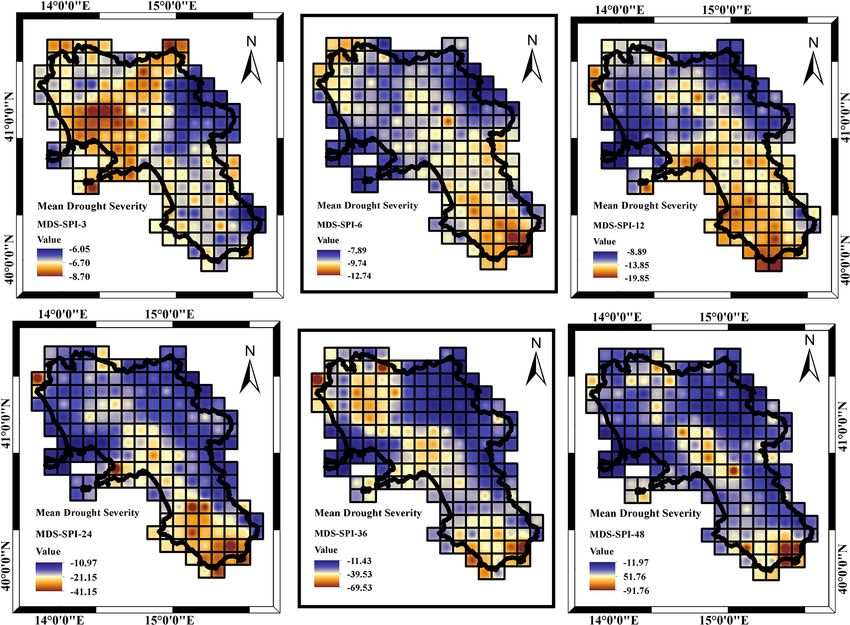
2182                                          A. Longobardi et al.: Assessment of centennial (1918–2019) drought features

quently inadequate for drought characterization analysis. Be-     dent differences depending on the location (Longobardi and
yond ground rainfall observations, data from global weather       Villani, 2010; Longobardi and Mautone, 2015; Longobardi
datasets can be considered, but their coarse spatial resolution   et al., 2016; Longobardi and Boulariah, 2021). Two distinct
makes them poorly effective especially in capturing the high      rain gauge networks are available for the region: one for the
precipitation variability that affects the southern European      period 1918–1999 and the other for the period 2000–2019.
region. In this context, historical in situ long-term measure-    They are characterized by different stations’ consistency, lo-
ments are crucial for understanding historical drought condi-     calization and typology. With the aim of reconstructing con-
tions as they allow us to learn about how a specific region       tinuous long-term monthly scale precipitation time series, the
has been affected by precipitation shortage periods in the        in situ point measurements (observed at the rain gauge loca-
past, how severe the response was and how quickly it took         tions) for the two datasets were projected on a 10×10 km res-
to recover from drought conditions (Bonaccorso and Aron-          olution grid covering the whole region by using a geostatis-
ica, 2016; Marini et al., 2019). This information is important    tical interpolation approach (Boulariah et al., 2020). Project-
to set drought forecasting strategies which could help in pre-    ing the two distinct database point measurements to a com-
paredness actions, planning mitigation and adaptation strate-     mon grid made it possible to reconstruct centennial monthly
gies to projected climate change (Peres et al., 2020; Gaitán      precipitation time series from 1918 to 2019, which is crucial
et al., 2020).                                                    for long-term historical drought condition analysis.
   One of the widely used approach to define drought con-            The reconstructed gridded precipitation database was used
ditions and persistence consists in the use of mathematical       to compute the Standardized Precipitation Index at different
indices, known as drought indicators, such as the Palmer          accumulation time steps, from SPI_3 to SPI_48, to explore
Drought Severity Index (PDSI) (Palmer, 1965), the Crop            the full range of drought definitions. SPI time series were an-
Moisture Index (CMI) (Palmer, 1968), the Normalized Dif-          alyzed for their spatial and temporal patterns features, and
ference Vegetation Index (NDVI) (Rouse et al., 1974), the         the modified Mann–Kendall and the Sen’s slope tests were
Standardized Precipitation Index (SPI) (McKee et al., 1993;       used to assess the trend significance and magnitude. Addi-
Ganguli and Reddy, 2014), the Drought Recognition In-             tionally, the spatial patterns of drought characteristics were
dex (RDI) (Tsakiris and Vangelis, 2005) and the Standard-         evaluated with the assessment of probability of occurrence,
ized Precipitation Evapotranspiration Index (SPEI) (Vicente-      drought duration, drought severity and drought peak value
Serrano et al., 2010). In particular the SPI, despite the in-     for different SPI thresholds, according to the run theory (Yev-
herent limitations, was used in several studies to investigate    jevich, 1967).
drought characteristics across the world (Mishra and Singh,          The findings of the study in terms of detailed spatial and
2010; Van Loon, 2015).                                            temporal characterization of drought conditions within the
   Concerning the Italian territory, Capra et and Sci-            Campania region represent essential information for sus-
colone (2012) investigated the spatiotemporal variability of      tainable and efficient water resource management planning
drought at short and medium accumulation scales in the            strategies.
Calabria region, southern Italy, using the SPI index, con-
cluding that approximately half of the region was impacted
by drought during the period 1981–1990 when the region            2     Material and methods
suffered its worst drought. Di Lena et al. (2014) analyzed
drought periods in the Abruzzo region, showing a gen-             2.1    Study area
eral downward trend in SPI time series which were more
pronounced on longer accumulation timescales. Marini et           The Campania region is located between 40.0 and 41.5◦ N
al. (2019) investigated droughts in the Apulia region using       and 13.5 and 16.0◦ E, covering about 13 600 km2 in the
the SPI and the RDI indices, finding an upward trend in the       southwest of Italy (Fig. 1).
severity of droughts in the western part and a downward trend        The region is well known for a complex orography; the
in the eastern region. By applying the SPI index over 3 and       altitude of the region ranges from well above 2000 m a.s.l.
6 months for a short-term analysis and 12 and 24 months for       (above sea level) in the Apennine Mountains to the coastline.
a long-term analysis, Caloiero et al. (2018) analyzed dry and     The region is characterized by a complex climatic pattern be-
wet periods in southern Italy, showing that when long-term        cause of the orography. The seasonality is well defined, with
precipitation scales are included, the probabilities of occur-    the larger amount of precipitation recorded during the winter
rence of dry conditions are higher than the wet ones.             periods. The mean annual rainfall of the study area ranges
   The reported case study is represented by the Campania         from 600 to 2400 mm, whereas the average annual temper-
region, located in southern Italy, which is a large area of       ature is around 17 ◦ C. Trends in historical precipitation and
about 13 600 km2 stretching from the Apennine Mountains           their seasonal variability were described in Longobardi and
to the Mediterranean Sea with progressively decreasing ele-       Villani (2010) and Longobardi et al. (2016). The area is ex-
vations moving from the inland to the coastline. The climate      periencing a moderate negative trend in precipitation, espe-
regime of the study area is typically seasonal with some evi-     cially concerning the northeastern and southwestern areas.

Nat. Hazards Earth Syst. Sci., 21, 2181–2196, 2021                               https://doi.org/10.5194/nhess-21-2181-2021
A. Longobardi et al.: Assessment of centennial (1918–2019) drought features                                                         2183

Figure 1. The studied area. (a, b) The two rain gauge networks. (c) The study area in the red box. (d) The grid shape for the region under
investigation. Red boxes represent grid cells no. 2 and no. 108 reported in Fig. 3.

At the same time, the seasonal variability also appeared to be         tially interpolated by the co-kriging, which was found to be
featured by a negative trend, with a transition of the precipi-        the best interpolating method over the investigated area based
tation regime from a seasonal to more uniform one.                     on the results of an interpolation approach comparative study,
                                                                       due to the high correlation (≥ 70 %) between elevation and
2.2   Dataset                                                          observed precipitation (Boulariah et al., 2020). The interpo-
                                                                       lated precipitation fields (for each month and for each year)
As mentioned in the introduction, the gridded datasets used            were projected on a high-resolution grid base (10 × 10 km).
in the current paper were obtained from the research carried           The result of the merging process was monthly gridded rain-
out by Boulariah et al. (2020), in which different spatial in-         fall data from 1918 to 2019 for 191 high-resolution grid
terpolation approaches (both deterministic and geostatistical          points covering the whole of the Campania region, which
approaches) were applied to merge two monthly precipita-               were considered for the proposed analysis (Fig. 1c).
tion rain gauge (point) databases available for the studied re-
gion; they are different in rain gauge locations and moreover          2.3   The Standardized Precipitation Index
cover different periods of time, one referring to the period
1918–1999 and the second to 2000–2019 (Fig. 1a and b). The             The formulation of the SPI drought index for any given loca-
number of available rain gauge stations were 154 and 187 re-           tion is based on the cumulative rainfall record over a selected
spectively for the first period and the second period. Compar-         timescale and the probability density function “Gamma”,
ing the two considered periods of time, rain gauge density is          which fit only positive and null values (McKee et al., 1993;
then rather similar and rain gauge stations are similarly dis-         Husak et al., 2007). In the literature and according to pre-
tributed over the region, with an exception for the Sorrento           vious studies, the rainfall time series are first fitted to the
Peninsula, a coastline area at the middle latitudes of the re-         Gamma distribution and then standardized by transformation
gion. The two-point dataset (rain gauge dataset) were spa-             into a normal distribution (Caloiero et al., 2018; Martinez et

https://doi.org/10.5194/nhess-21-2181-2021                                     Nat. Hazards Earth Syst. Sci., 21, 2181–2196, 2021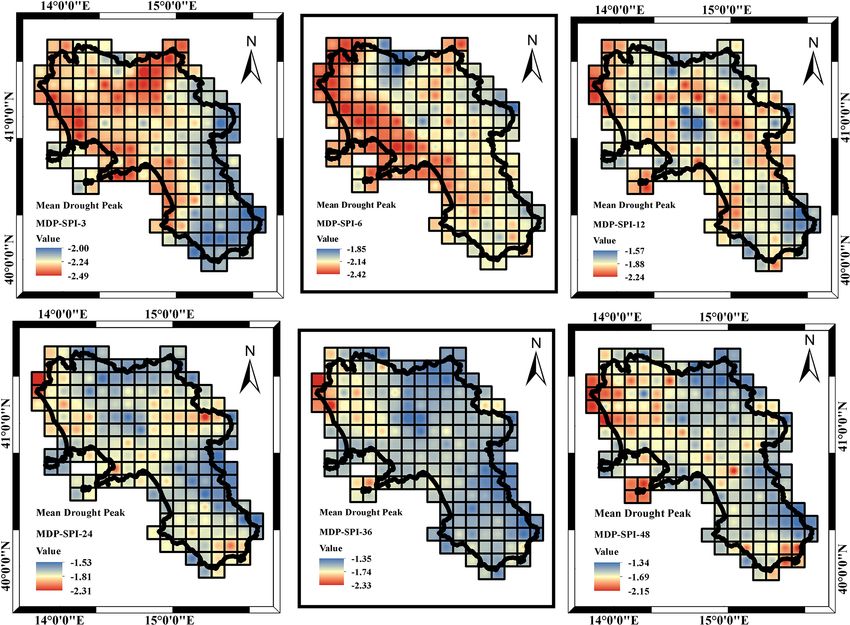
2184 A. Longobardi et al.: Assessment of centennial (1918–2019) drought features
al., 2019; Stagge et al., 2015; Zhou and Liu, 2016). The prob- Table 1. Classification of wet and dry conditions according to SPI
ability density function for the Gamma distribution can be values (McKee et al., 1993).
expressed by the following equation:
SPI Values Drought severity
1
g(x) = α x α−1 e−x/β , (1) SPI ≥ 2.0 Extremely wet
β 0(α)
1.5 ≤ SPI < 2.0 Very wet
where α, β and x are respectively the shape parameter, the 1.0 ≤ SPI < 1.5 Moderately wet
scale parameter and the amount of precipitation (α, β and −1.0 < SPI < 1.0 Near normal
x > 0). 0(α) is the gamma function expressed as follows: −1.5 < SPI ≤ −1.0 Moderately dry
Z ∞ −2.0 < SPI ≤ −1.5 Severely dry
0(α) = y α−1 e−y dy. (2) SPI < −2.0 Extremely dry
0
Parameters α̂ and β̂ are assessed through the maximum like-
lihood method (McKee et al., 1993; Liu et al., 2016): SPI_24, SPI_36 and SPI_48) were computed for the studied
r ! dataset and used to describe wet and dry conditions accord-
1 4A x ing to the values reported in Table 1 (McKee et al., 1993).
α̂ = 1+ 1+ and β̂ = , (3)
4A 3 α̂
2.4 Trend analysis
where
P
ln(x) Time series of SPI were tested for trend detection in time.
A = ln(x) − (4)
n A trend is a significant change over time exhibited by a ran-
for n observations. By integrating the density of probability dom variable, detectable by statistical parametric and non-
function g(x), the cumulative probability G(x) is obtained: parametric procedures. Provided the intrinsic autocorrela-
tion of the analyzed time series, the current study provided
Zx Zx results for non-parametric modified Mann–Kendall (MMK)
1 − βx
G(x) = g(x)dx = = x α̂−1 e dx. (5) and Sen’s test approaches. Those methods are briefly de-
β̂0(α̂)
0 0 scribed in the following.
Given that the Gamma distribution is not defined for x values The Mann–Kendall test (Mann, 1945; Kendall, 1962) is
equal to zero and that instead the cumulative rainfall series one of the most widely used methods to detect trend in cli-
may contain null values, the cumulative distribution is re- matology analysis. It is used to analyze data collected over
defined as follows: time for consistently increasing or decreasing trends (mono-
tonic). It is a non-parametric test, which means it works for
H (x) = q + (1 − q)G(x), (6) all distributions; thus tested data do not have to meet the as-
where q is the probability of zero precipitation. Then, the sumption of normality but should have no serial correlation.
value of the SPI can be obtained through the approximation The Mann–Kendall statistic S is defined as follows:
proposed in Abramowitz and Stegun (1964) which converts n−1 X
X n
the cumulative distribution H (x) to a normal random vari- S= sign(xj − xi ), (9)
able Z: i=1 j =i+1
Z = SPI where
− t − c0 +c1 t+c2 2 t 2 3 , for 0 < H (x) ≤ 0.5
1+d 1 t+d 2 t +d t
3 +1, if (xj − xi ) > 1
= ,
+ t − c0 +c1 t+c2 2 t 2 3 , for 0.5 < H (x) ≤ 1 sign(xj − xi ) = 0 , if (xj − xi ) = 0 , (10)
1+d t+d t +d t
1 2 3
−1, if (xj − xi ) < 1
(7)
where xi and xj are the annual values in years i and j , with
r h i
1
ln (H (x)) 2 , for 0 < H (x) ≤ 0.5
i > j . When n ≥ 10, the statistic S is almost normally dis-
t= r h i , (8) tributed with mean E(S) and variance Var(S) as follows:
ln (1−H1(x))2 ,
for 0.5 < H (x) ≤ 1
n(n − 1)(2n + 5)
E(S) = 0, Var(S) = . (11)
where 18
c0 = 2.515517, c1 = 0.802853, c2 = 0.010328, However, the expression of Var(S) should be adjusted when
d0 = 1.432788, d1 = 0.189269, d2 = 0.001308. tied values do exist:
" q
#
SPI time series for different accumulation periods of 3, 6, 12, 1 X
Var(S) = n(n − 1)(2n + 5) − tp (tp − 1)(2tp + 5) , (12)
24, 36 and 48 months (respectively SPI_3, SPI_6, SPI_12, 18 p=1
Nat. Hazards Earth Syst. Sci., 21, 2181–2196, 2021 https://doi.org/10.5194/nhess-21-2181-2021
A. Longobardi et al.: Assessment of centennial (1918–2019) drought features 2185
where q is the number of tied groups and tp is the number of
data values in the pth group. The standardized test statistic
Z follows a standard normal distribution and is computed as
follows:
S−1
√Var(S) if S > 0
Z= 0 if S = 0 . (13)
√S+1
if S < 0
Var(S)
At the significance level α, the existing trend is considered to
be statistically significant if p ≤ α/2 in the case of the two-
tailed test.
To take into account the presence of autocorrelation in the
SPI time series, which might increase the probability to de-
tect trends when actually none exist, the modified Mann–
Kendall test can be applied (Hamed and Rao, 1998). Fur- Figure 2. Drought characteristic identification using the “run the-
thermore, the reason for the use the modified Mann–Kendall ory” (Yevjevich, 1967).
test (MMK) lays in its accuracy for the analysis of correlated
data (Hamed and Rao, 1998; Mondal et al., 2012; Sa’adi
et al., 2019), which is the case for the SPI time series in 2.5 Drought characteristics
this study, compared to the original Mann–Kendall trend test
To describe meteorological drought features of the studied
without any loss of power. For this purpose, a modified form
area, the occurrence of drought events was evaluated for each
of Var(S), set as Var(S)∗ , is used as follows:
cell of the gridded dataset according to the SPI threshold,
n and the average over the period of observation was illus-
Var(S)∗ = Var(S) ∗ , (14)
n trated. Two different thresholds in the SPI value were used,
where n∗ is the effective sample size and n the number of SPI ≤ −1 and SPI ≤ −2, to detect the behavior of the region
observations. The ratio between the effective sample size and with respect to moderate and extremely severe drought con-
the actual number of observations was computed as proposed ditions (see Table 1). The effect of the accumulation period
by Hamed and Rao (1998) as follows: was investigated.
n−1
Additionally, three drought characteristics, namely mean
n 2 X
drought duration (MDD), mean drought severity (MDS) and
= 1 +
n∗ n(n − 1)(n − 2) i=1 mean drought intensity (MDP) (Guo et al., 2018; Wang et
al., 2019; Fung et al., 2020), were selected. By linking the
(n − i)(n − i − 1)(n − i − 2)ri , (15)
SPI data with the “run theory” proposed by Yevjevich (1967)
where ri is the lag-i significant auto-correlation coefficient and according to Wang et al. (2019), MDD and MDS were
of rank i of the time series. calculated as follows:
Sen (1968) developed a non-parametric procedure to as- PN
sess the slope of trend in a sample of N pairs of data: DDi
MDD = i=1 , (18)
xj − xi N
Qi = , i = 1, 2, . . .Nj > i, (16) PN
j −i DSi X
MDS = i=1 , DSi = DDi
SPI, (19)
N
where xj and xi are data values at time j and i (j > i) re-
spectively. If there is only one datum in each time period, where, provided a given SPI threshold, DD is the period of
then N = n(n − 1)/2, where n is the number of time peri- time with continuous (negative) values of the SPI below the
ods. If there are multiple observations in one or more time given threshold (i.e. drought spell duration in the run the-
periods, then N = n(n − 1)/2, where n is the total number of ory), i is the number of the sequence of DD, N is the total
observations. number of drought spells observed during the studied period,
The N values of Qi are ranked from smallest to largest, and DSi is the value of drought severity associated with the
and the median of slope or Sen’s slope estimator is computed period DDi (Fig. 2). Events with DD ≥ 3 months were only
as accounted for. Additionally, the mean drought intensity MDP
(
Q N +1 if N is odd
) was computed as the ratio between MDS and MDD (Li et al.,
Qmed = h 2 i . (17) 2017). As in the case of the computation of MDD, MDS and
1
2 Q N + Q N +2 if N is even MDP, the two different thresholds, SPI ≤ −1 and SPI ≤ −2,
2 2
were taken into consideration. The effects of the accumula-
The Qmed sign reflects the data trend behavior (increase or
tion scale and the spatial patterns were investigated.
decrease), while its value indicates the steepness of the trend.
https://doi.org/10.5194/nhess-21-2181-2021 Nat. Hazards Earth Syst. Sci., 21, 2181–2196, 2021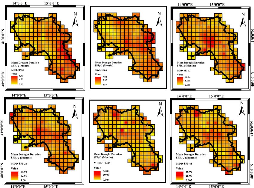
2186 A. Longobardi et al.: Assessment of centennial (1918–2019) drought features
Figure 3. SPI_6, SPI_12 and SPI_24 for cell no. 2 (southern area – a, c, e) and cell no. 108 (northern area – b, d, f).
3 Results and discussion Starting from the SPI_3 to SPI_12, the downward trend
become dominant in the study area and is especially marked
3.1 Temporal analysis in the northwestern and southern sectors of the region
(Fig. 4), which correspond to the area featured by the largest
The temporal patterns of the SPI time series in the region mean annual precipitation and the largest precipitation down-
under investigation at different timescales have the potential ward trend (Longobardi and Villani, 2010). The proportion
to provide insights into the temporal variation of droughts in of negative to positive trends, with negative values still dom-
the Campania region. As an example, Fig. 3 illustrates SPI_6, inant in over 60 % of the cells, remains almost similar for the
SPI_12 and SPI_24 for two cells of the grid data (Fig. 1). In SPI_24 to SPI_48.
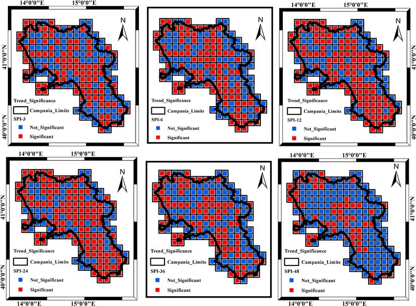
the left panels an example from the southern coastal area is Concerning the significance of the trend (Fig. 5), the
depicted, whereas in the right panels the example is from the MMK test illustrated how a very large proportion of the
northern inland area. gridded SPI showed a significant trend over the different
In both areas, Fig. 3 clearly highlights the drought peri- timescales especially from the SPI_3 to the SPI_24 accumu-
ods that affected the Campania region around 1940–1950 lation scale (Fig. 5). For the SPI_3, SPI_6 and SPI_12, the
and around 1990–2010. This result appears consistent with negative trend is particularly significant, with a percentage
a European-scale assessment study in which it was reported of grid cells of about 55 % for both SPI_3 and SPI_6 and
that the period between 1985 and 1995 was characterized by 65 % for SPI_12. Regarding the spatial distribution of the
the broadest spread of extreme drought events, mainly local- trend, the SPI_24 is the most significant with almost 70 % of
ized on the Iberian Peninsula, southern Europe, the Balkans the grid cells. Beyond this scale, temporal variations did not
and western Turkey (Bonaccorso et al., 2013). Drought appear significant. As the groundwater systems of the region
severity appears less pronounced in the northern inland areas, are characterized by long delay times and thus being poten-
especially if looking at the longest accumulation timescale. tially impacted by SPI accumulated over a large scale, it is
Drought tends to be more persistent in the southern areas than likely that those systems are not strongly impacted by cli-
in northern ones which additionally have been only impacted mate temporal variations (Longobardi and Van Loon, 2018).
a little by the drought conditions starting in 2015 in the re- On the national scale, the obtained results were well in line
gion. More details about the spatial variability of drought fea- with the general overview outlined in previous research by
tures will be discussed in the following. Delitala et al. (2000) and Bordi et al. (2001) for other regions
The modified Mann–Kendall (MMK) test and the Sen’s of southern Italy (Sardinia, Sicily and Puglia) and, further-
slope estimator were carried out to investigate temporal more, were in perfect accord with the outcomes given by
trends, sign, significance and magnitude in SPI time series Buttafuoco and Caloiero (2014) for the Calabria region in
over the studied period. The relevant results of the MMK southern Italy.
for trend sign and significance (significance level = 5 %) are At the regional scale, the results for the modified Mann–
shown respectively in Figs. 4 and 5. Kendall trend test are also consistent with the findings of pre-
Nat. Hazards Earth Syst. Sci., 21, 2181–2196, 2021 https://doi.org/10.5194/nhess-21-2181-2021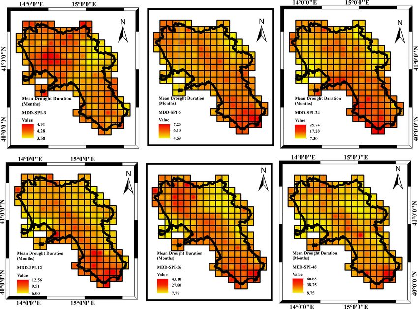
A. Longobardi et al.: Assessment of centennial (1918–2019) drought features                                                 2187

Figure 4. SPI MMK test sign for the different accumulation scales (α = 5 %).

Figure 5. SPI MMK test significance (α = 5 %) for the different accumulation scales.

https://doi.org/10.5194/nhess-21-2181-2021                                     Nat. Hazards Earth Syst. Sci., 21, 2181–2196, 2021
2188                                             A. Longobardi et al.: Assessment of centennial (1918–2019) drought features

Figure 6. SPI Sen’s slope for the different accumulation timescales.

vious climatological studies concerning precipitation regime           3.2   Drought characteristics assessment
investigation (Longobardi and Villani, 2010; Longobardi et
al., 2016). In fact, annual and seasonal precipitation in the          Figure 7 shows the total number of drought events detected
region were found to be featured by a generalized negative             within the SPI time series from 1918 to 2019 for moder-
trend during the last century, even though the downward ten-           ate drought conditions (threshold SPI ≤ −1) and for ex-
dencies, contrary to the SPI tendencies, were significant for          tremely severe drought conditions (threshold SPI ≤ −2) for
a very moderate number of rain gauge stations.                         each point of the grid for all the accumulation scales con-
   The magnitude of the trend in the SPI time series, as as-           sidered. In the case of moderate drought events, it was ob-
sessed using Sen’s estimator, is presented in Fig 6. In agree-         served that the SPI_3 is associated with the largest number
ment with the results of the MMK test, the trend was dom-              of droughts, which was on average 95, for the whole period
inantly negative across the region, which is consistent with           of observation over the 191 grid cells. Provided the large the-
the trend sign represented in Fig. 4 with some exceptions for          oretical autocorrelation in SPI time series for the larger ac-
a west–east transect at the middle latitudes of the region that        cumulation scale, drought frequency decreased with increas-
correspond to an area which features moderate mean annual              ing accumulation scale, with the SPI_24 to SPI_48 patterns
precipitation values and the lowest downward precipitation             almost similar among them (Fig. 7 upper panel). The re-
trends (Longobardi and Villani, 2010). On average, the ten-            sults appeared in good agreement with those demonstrated
dency toward drier conditions was however rather moderate              by other authors (McKee et al., 1993; Buttafuoco et al., 2015;
and characterized by an amplification with increasing accu-            Marini et al., 2019; Fung et al., 2020). A very similar be-
mulation timescale. The increase in the SPI index amounts              havior was found in the case of extremely severe drought
to about 10 % in 10 years for the case of SPI_6. It increases          episodes except for the lower number compared to the case
up to 15 % and 24 % in 10 years respectively for the case              of moderate events. The average number of drought events
of SPI_12 and SPI_48. The variability in the minimum and               in the case of SPI_3 for the threshold SPI ≤ −2 was on av-
maximum assessed trend, on the spatial scale, also increases           erage 27 for the whole period of observation over the 191
for increasing accumulation timescale.                                 grid cells. Concerning the spatial patterns, although a moder-
                                                                       ate correlation appeared for small cluster of cells, an evident
                                                                       concentration of drought event occurrence in a specific area
                                                                       was not found.

Nat. Hazards Earth Syst. Sci., 21, 2181–2196, 2021                                    https://doi.org/10.5194/nhess-21-2181-2021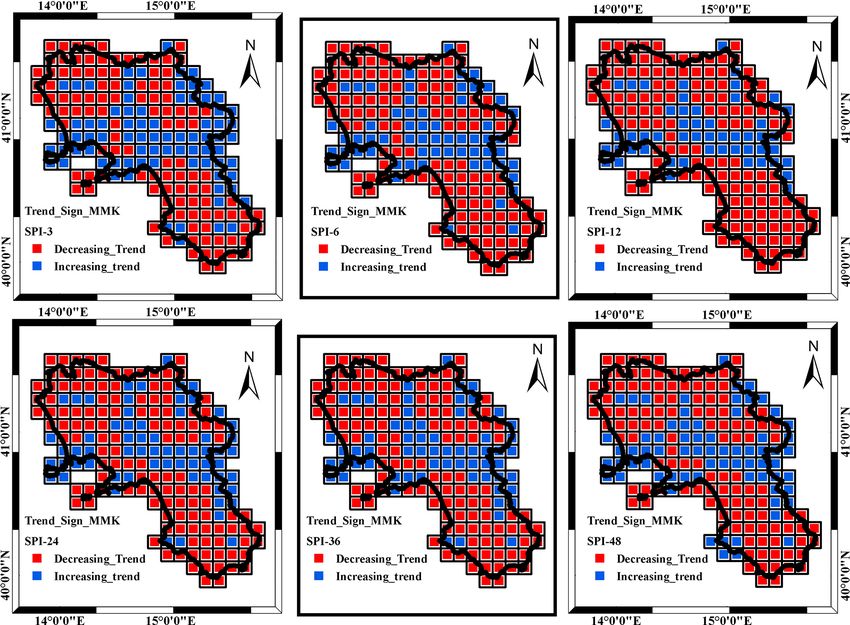
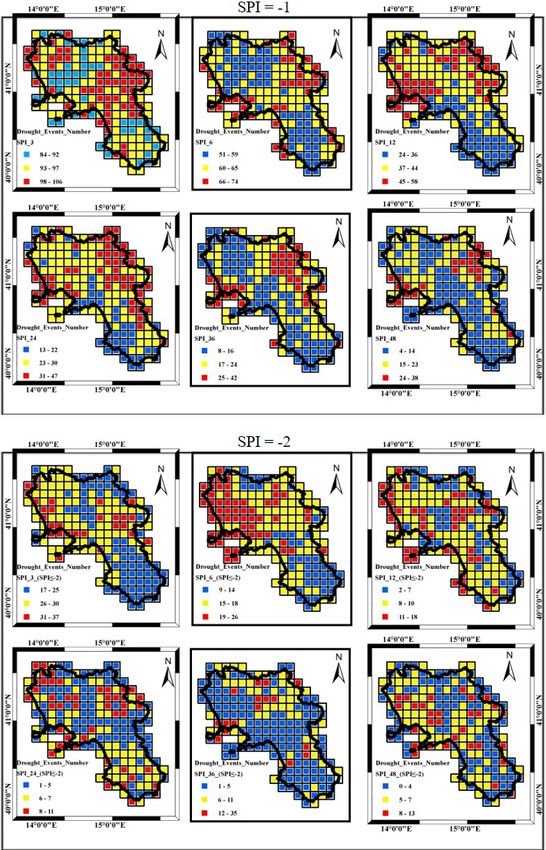
A. Longobardi et al.: Assessment of centennial (1918–2019) drought features                                                 2189

Figure 7. Number of drought events for the different accumulation timescales over the whole period of observation 1918–2019. Upper
panels: moderate drought events (SPI ≤ −1). Lower panels: extremely severe drought events (SPI ≤ −2).

https://doi.org/10.5194/nhess-21-2181-2021                                Nat. Hazards Earth Syst. Sci., 21, 2181–2196, 2021
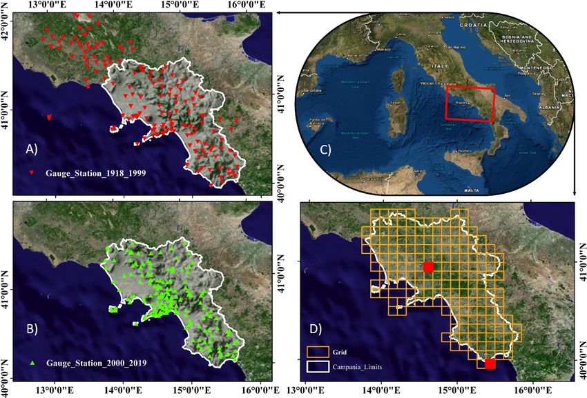
2190                                           A. Longobardi et al.: Assessment of centennial (1918–2019) drought features

Figure 8. MDD (mean drought duration) for the different accumulation periods considered (SPI ≤ −1).

Figure 9. MDS (mean drought severity) for the different accumulation periods considered (SPI ≤ −1).

Nat. Hazards Earth Syst. Sci., 21, 2181–2196, 2021                                    https://doi.org/10.5194/nhess-21-2181-2021
A. Longobardi et al.: Assessment of centennial (1918–2019) drought features                                                 2191

   More insights came from the analysis of the MDD, MDS               With reference to the MDS and consequently to the
and MDP respectively illustrated in Figs. 8, 9 and 10 with         MDD, the drought severity increased with the accumula-
reference to a threshold value of SPI ≤ −1.                        tion timescale ranging from 16 for the SPI_3 to 109 for the
   Concerning the MDD (Fig. 8), different from what oc-            SPI_48 (Fig. 12). Compared to the case of moderate drought
curred in terms of drought frequency, the mean drought du-         events, in the case of extremely severe events the mean
ration increased with the accumulation timescale, ranging          drought severity increased for each accumulation scale. Con-
from 4 to 5 months for the SPI_3 to 8 to 60 months for the         cerning the spatial pattern of MDS, it appeared as a common
SPI_48. The accumulation timescale also affected the MDD           feature according to which the largest MDS values appeared
spatial behavior (Fig. 8). In the case of SPI_3 and SPI_6,         in the central area of the region, with some spot cells located
almost the whole region was affected by the average MDD            in the extremely southern and extremely northern coastlines.
values. In the case of SPI_12, SPI_24, SPI_36 and SPI_48,          An exception was provided by the lower SPI_3.
the largest MDD values were detected along a northwest to             In the end, concerning the MDP (Fig. 13), different to
southeast transect and more evidently in the southern sectors      what occurred in the case of the MDD and MDS, the min-
of the region. At the smallest timescales (SPI_3) the northern     imum (about −2.5 on average) and maximum (about −3.5
sections are the most impacted. For the longer accumulation        on average) values appeared similar for the different ac-
timescales, the maximum values detected in the southern re-        cumulation timescales and likely more pronounced for the
gion were mainly caused by severe drought periods which            lower accumulation scales (−4.09 for SPI_6). The spatial
occurred in 1990, 2003 and 2017 in the region.                     pattern was found to be particularly complex and did not
   Concerning the MDS (Fig. 9), because of the MDD char-           show a clear tendency related to the accumulation timescale
acteristics, the drought severity increased with the accumu-       (Fig. 13). Larger peaks were still focused in the central area
lation timescale ranging from 6 to 8 for the SPI_3 to 11 to        of the region, but the area covered changed with accumula-
90 for the SPI_48 (Fig. 9). The spatial pattern of MDS was         tion timescale, being rather moderate for the larger SPI ac-
affected by the accumulation timescale, such as in the case of     cumulation scale. A large peak appeared to spread all over
the MDD. For the SPI_3, MDS showed a major severity in             the region in the case of the largest accumulation periods,
the northern area, whereas moving from SPI_12 to SPI_48,           SPI_36 and SPI_48.
MDS severity moved from northern to southern areas and al-
most disappeared with an even distribution set at an almost
constant value (about −10).                                        4   Conclusions
   Concerning the MDP (Fig. 10), because of what was pre-
viously observed in the case of the MDD and MDS, the min-          Drought is a sustained period of below-normal water avail-
imum (about −1.5 on average) and maximum (about −2.3               ability. It is a recurring and worldwide phenomenon, but the
on average) values appeared similar for the different accu-        Mediterranean Basin is seen as a very vulnerable environ-
mulation timescales and were likely more pronounced for the        ment in this perspective. The main objective of this study
lower accumulation scales where MDP’s largest peaks are fo-        was to assess the drought features in the Campania region of
cused on the northern area. In contrast, the spatial pattern was   southern Italy through an analysis of the spatial and temporal
found to be particularly complex and did not show a clear          pattern characteristics of SPI time series, computed at differ-
tendency related to the accumulation timescale (Fig. 10).          ent accumulation scales over a centennial period from 1918
Overall, the largest peaks are detected in the northern areas      to 2019. The modified Mann–Kendall test and the Sen’s test
of the region for the SPI_3 to SPI_6. From SPI_24 to SPI_48        were applied to describe the temporal trend significance and
there was a general tendency for a dominant low peak spatial       magnitude. Additionally, for both moderate (SPI ≤ −1) and
distribution, with an exception for some coastline areas in the    extremely severe (SPI ≤ −2) drought conditions, the “run
north of the region. The SPI_12 represented a neutral condi-       theory” (Yevjevich, 1967) was applied to illustrate drought
tion, where minimum and maximum SPI values are rather              events frequency, duration, peak and severity.
pronounced and spread over the region.                                Concerning the drought temporal features, the trend was
   By increasing the threshold for the SPI values, moving          found to be dominantly negative, and the percentage of im-
from SPI ≤ −1 to SPI ≤ −2, it was possible to explore the          pacted cells increased with accumulation scale. It remained
extremely severe drought conditions over the region.               almost similar for SPI time series computed over 24 months
   Concerning the MDD (Fig. 11), the mean drought dura-            or longer intervals. The significance was also found to be par-
tion increased with the accumulation timescale, ranging from       ticularly evident approaching 70 % of grid cells for SPI_24.
3 months for the SPI_3 to 47 months for the SPI_48. Com-           Beyond this timescale threshold, significance in temporal
pared to the case of moderate drought events, in the case of       variability strongly decreased. The SPI increase over time,
extremely severe events the mean drought duration decreased        ranging from about 10 % in 10 years for the case of SPI_6
for each accumulation scale. Concerning the spatial distri-        and 24 % for the SPI_48. In the case of moderate dry condi-
bution, the same consideration provided for the case of SPI        tions, MDD increased with the accumulation timescale, rang-
threshold ≤ −1 hold also in the case of SPI threshold ≤ −2.        ing from about 5 months for the SPI_6 to 60 months for

https://doi.org/10.5194/nhess-21-2181-2021                                Nat. Hazards Earth Syst. Sci., 21, 2181–2196, 2021
2192                                           A. Longobardi et al.: Assessment of centennial (1918–2019) drought features

Figure 10. MDP (mean drought peak) for the different accumulation periods considered (SPI ≤ −1).

Figure 11. MDD (mean drought duration) for the different accumulation periods considered (SPI ≤ −2).

Nat. Hazards Earth Syst. Sci., 21, 2181–2196, 2021                                   https://doi.org/10.5194/nhess-21-2181-2021
A. Longobardi et al.: Assessment of centennial (1918–2019) drought features                                               2193

Figure 12. MDS (mean drought severity) for the different accumulation periods considered (SPI ≤ −2).

Figure 13. MDP (mean drought peak) for the different accumulation periods considered (SPI ≤ −2).

https://doi.org/10.5194/nhess-21-2181-2021                                   Nat. Hazards Earth Syst. Sci., 21, 2181–2196, 2021
2194                                              A. Longobardi et al.: Assessment of centennial (1918–2019) drought features

the SPI_48. Accordingly, MDS increased with accumulation               RESTORE). Data will be available, upon request, at https://www.
scale, moving from about −10 in the case of SPI_6 to about             progettorestore.it (last access: July 2021) (RESTORE, 2021).
−50 in the case of SPI_48. MDP did not change significantly
with the accumulation scale and was particularly pronounced
in the case of the shorter temporal scales. Extremely severe           Author contributions. AL and PV contributed to the conceptualiza-
events were featured by shorter durations and larger severity          tion. AL and OB contributed to data curation and formal analysis.
compared to the moderate drought events but were much less             AL and PV provided supervision, and AL and OB wrote the orig-
                                                                       inal draft. AL, OB and PV contributed to the revised manuscript
frequent (over 75 % less then).
                                                                       version.
   Concerning the spatial pattern, the negative trends ap-
peared to occur along a northwest to southeast transect,
whereas positive trends were focused along a west–east tran-           Competing interests. The authors declare that they have no conflict
sect at the middle latitude of the region. These areas are re-         of interest.
spectively featured by large mean annual precipitation cou-
pled with the largest negative trends and by low to mod-
erate mean annual precipitation and lowest negative trends.            Disclaimer. Publisher’s note: Copernicus Publications remains
Those two regions are quite different in terms of orogra-              neutral with regard to jurisdictional claims in published maps and
phy. While the first is characterized by mountainous relief            institutional affiliations.
approaching or close to the coastline, the second features a
large plain devoted to agricultural practices, crossed by the
longest river of the region, the Volturno River, which proba-          Special issue statement. This article is part of the special issue “Re-
bly represents an access corridor to atmospheric weather sys-          cent advances in drought and water scarcity monitoring, modelling,
tems. The complex orography of the region appears then to              and forecasting (EGU2019, session HS4.1.1/NH1.31)”. It is a re-
impact both the average precipitation spatial distribution and         sult of the European Geosciences Union General Assembly 2019,
the relevant temporal variability. The accumulation timescale          Vienna, Austria, 7–12 April 2019.
affected the MDD spatial behavior. At the lowest accumula-
tion scale, the northern area appeared to be more affected,
                                                                       Acknowledgements. The authors would like to thank the anony-
whereas large MDD values were detected along a northwest
                                                                       mous referees for their encouragement and helpful comments which
to southeast transect and were however more evident in the
                                                                       resulted in an improved manuscript version and the “Centro Fun-
southern sectors of the region. The maximum values detected            zionale Multirischi della Protezione Civile Regione Campania” for
in the southern area for the longer accumulation timescale             providing the observed precipitation data. Furthermore, the authors
were mainly caused by severe drought periods occurring in              would like to thank Valentina Nobile and Marco Sessa for their ef-
1990, 2003 and 2017 in the region. The MDS spatial pattern             fective support in data collection.
was also affected by accumulation scale. It showed a con-
centration on the northern region area for the shorter tem-
poral scales and instead a constant spatial distribution for           Review statement. This paper was edited by Brunella Bonaccorso
the longer temporal scales, with an exception for a north-             and reviewed by two anonymous referees.
west to southeast transect and for the southern sectors of the
region where the largest MDS values were detected. In the
end, the MDP spatial pattern was found to be particularly
                                                                       References
complex and did not show a clear tendency related to the ac-
cumulation timescale. At least for the shorter timescale, the          Abramowitz, M. and Stegun, I. A.: Handbook of mathematical func-
largest drought peaks seemed concentrated on the norther in-             tions with formulas, graphs, and mathematical tables, US Gov-
land area of the region, which overall could be addressed as             ernment printing office, 1964.
an area potentially prone to agricultural drought stress.              Bonaccorso, B. and Aronica, G. T.: Estimating Temporal Changes
   The current research illustrated how historical in situ long-         in Extreme Rainfall in Sicily Region (Italy), Water Resour.
term measurements are crucial for understanding historical               Manag., 30, 5651–5670, 2016.
drought conditions to plan mitigation strategies to further            Bonaccorso, B., Peres, D. J., Cancelliere, A., and Rossi, G.: Large
face future climate change impacts.                                      Scale Probabilistic Drought Characterization Over Europe, Wa-
                                                                         ter Resour. Manag., 27, 1675–1692, 2013.
                                                                       Bordi, I., Frigio, S., Parenti, P., Speranza, A., and Sutera, A.: The
                                                                         analysis of the Standardized Precipitation Index in the Mediter-
Data availability. The presented research results are part of
                                                                         ranean area: regional patterns, Ann. Geophys.-Italy, 44, 5–6,
the RESTORE project (PSR 2014–2020 – TIPOLOGIA 16.5.1
                                                                         https://doi.org/10.4401/ag-3549, 2001.
“Azioni congiunte per la mitigazione dei cambiamenti climatici e
                                                                       Boulariah, O., Longobardi, A., Nobile, V., Sessa, M., and Villani,
l’adattamento ad essi e per pratiche ambientali in corso” – Progetto
                                                                         P.: Long term monthly precipitation database reconstruction for
                                                                         drought assessment, in: “ClimRisk2020: Time for Action! Rais-

Nat. Hazards Earth Syst. Sci., 21, 2181–2196, 2021                                      https://doi.org/10.5194/nhess-21-2181-2021
A. Longobardi et al.: Assessment of centennial (1918–2019) drought features 2195
ing the ambition of climate action in the age of global emergen- Husak, G. J., Michaelsen, J., and Funk, C.: Use of the gamma dis-
cies” – SISC Seventh Annual Conference, October 2020, online, tribution to represent monthly rainfall in Africa for drought mon-
21–23, 2020. itoring applications, Int. J. Climatol., 27, 935–944, 2007.
Buttafuoco, G. and Caloiero, T.: Drought events at different IPCC: Climate Change 2014: Synthesis Report, Contribution of
timescales in southern Italy (Calabria), J. Maps, 10, 529–537, Working Groups I, II and III to the Fifth Assessment Report of
2014. the Intergovernmental Panel on Climate Change, edited by: Core
Buttafuoco, G., Caloiero, T., and Coscarelli, R.: Analyses of Writing Team, Pachauri, R. K. and Meyer, L. A., IPCC, Geneva,
drought events in Calabria (southern Italy) using standardized Switzerland, 151 pp., 2014.
precipitation index, Water Resour. Manag., 29, 557–573, 2015. Kendall, M. G.: Rank correlation methods, Hafner Publishing Com-
Caloiero, T., Veltri, S., Caloiero, P., and Frustaci, F.: Drought pany, New York, 1962.
analysis in Europe and in the Mediterranean basin us- Li, X.-X., Ju, H., Sarah, G., Yan, C.-R., Batchelor, W. D., and
ing the standardized precipitation index, Water, 10, 1043, Liu, Q.: Spatiotemporal variation of drought characteristics in the
https://doi.org/10.3390/w10081043, 2018. Huang-Huai-Hai Plain, China under the climate change scenario,
Caloiero, T. and Veltri, S.: Drought assessment in the Sardinia Re- J. Integr. Agr., 16, 2308–2322, 2017.
gion (Italy) during 1922–2011 using the standardized precipita- Littell, J. S., Peterson, D. L., Riley, K. L., Liu, Y., and Luce, C. H.:
tion index, J. Appl. Geophys., 176, 925–935, 2019. A review of the relationships between drought and forest fire in
Capra, A. and Scicolone, B.: Spatiotemporal variability of drought the United States, Glob. Change Biol., 22, 2353–2369, 2016.
on a short–medium time scale in the Calabria Region (Southern Liu, Z., Wang, Y., Shao, M., Jia, X., and Li, X.: Spatiotemporal
Italy), Theor. Appl. Climatol., 110, 471–488, 2012. analysis of multiscalar drought characteristics across the Loess
Cook, B. I., Anchukaitis, K. J., Touchan, R., Meko, D. M., and Plateau of China, J. Hydrol., 534, 281–299, 2016.
Cook, E. R.: Spatiotemporal drought variability in the Mediter- Longobardi, A. and Boulariah, O.: Long term regional changes
ranean over the last 900 years, J. Geophys. Res.-Atmos., 121, in inter-annual precipitation variability in a Mediterranean area,
2060–2074, 2016. Theor. Appl. Climatol., in review, 2021.
Delitala, A. M., Cesari, D., Chessa, P. A., and Ward, M. N.: Precip- Longobardi, A. and Mautone, M.: Trend analysis of annual and sea-
itation over Sardinia (Italy) during the 1946–1993 rainy seasons sonal air temperature time series in southern Italy, in: Engineer-
and associated large-scale climate variations, Int. J. Climatol., 20, ing Geology for Society and Territory-Volume 3, Springer, 501–
519–541, 2000. 504, 2015.
Di Lena, B., Vergni, L., Antenucci, F., Todisco, F., and Mannocchi, Longobardi, A. and Van Loon, A. F.: Assessing baseflow index vul-
F.: Analysis of drought in the region of Abruzzo (Central Italy) nerability to variation in dry spell length for a range of catchment
by the Standardized Precipitation Index, Theor. Appl. Climatol., and climate properties, Hydrol. Process., 32, 2496–2509, 2018.
115, 41–52, 2014. Longobardi, A. and Villani, P.: Trend analysis of annual and sea-
Dracup, J. A., Lee, K. S., and Paulson Jr., E. G.: On the definition sonal rainfall time series in the Mediterranean area, Int. J. Cli-
of droughts, Water Resour. Res.,16, 297–302, 1980. matol., 30, 1538–1546, 2010.
Fung, K., Huang, Y., and Koo, C.: Assessing drought conditions Longobardi, A., Buttafuoco, G., Caloiero, T., and Coscarelli, R.:
through temporal pattern, spatial characteristic and operational Spatial and temporal distribution of precipitation in a Mediter-
accuracy indicated by SPI and SPEI: case analysis for Peninsular ranean area (southern Italy), Environ. Earth Sci., 75, 1–20, 2016.
Malaysia, Nat. Hazards, 103, 2071–2101, 2020. Mann, H. B.: Nonparametric tests against trend, Econometrica, 13,
Gaitán, E., Monjo, R., Pórtoles, J., and Pino-Otín, 245–259, 1945.
M. R.: Impact of climate change on drought in Marini, G., Fontana, N., and Mishra, A. K.: Investigating drought in
Aragon (NE Spain), Sci. Total Environ., 740, 140094, Apulia region, Italy using SPI and RDI, Theor. Appl. Climatol.,
https://doi.org/10.1016/j.scitotenv.2020.140094, 2020. 137, 383–397, 2019.
Ganguli, P. and Reddy, M. J.: Evaluation of trends and multivariate Martinez, C., Goddard, L., Kushnir, Y., and Ting, M.: Sea-
frequency analysis of droughts in three meteorological subdivi- sonal climatology and dynamical mechanisms of rainfall in the
sions of western India, Int. J. Climatol., 34, 911–928, 2014. Caribbean, Clim. Dynam., 53, 825–846, 2019.
Gouveia, C., Trigo, R. M., Beguería, S., and Vicente-Serrano, S. McKee, T. B., Doesken, N. J., and Kleist, J.: The relationship of
M.: Drought impacts on vegetation activity in the Mediterranean drought frequency and duration to time scales, in: Proceedings
region: An assessment using remote sensing data and multi-scale of the 8th Conference on Applied Climatology, 179–183, 1993.
drought indicators, Global Planet. Change, 151, 15–27, 2017. Mishra, A. K. and Singh, V. P.: A review of drought concepts, J.
Guo, H., Bao, A., Liu, T., Ndayisaba, F., Jiang, L., Kurban, A., and Hydrol., 391, 202–216, 2010.
De Maeyer, P.: Spatial and temporal characteristics of droughts in Mondal, A., Kundu, S., and Mukhopadhyay, A.: Rainfall trend anal-
Central Asia during 1966–2015, Sci. Total Environ., 624, 1523– ysis by Mann-Kendall test: A case study of north-eastern part of
1538, 2018. Cuttack district, Orissa, Int. J. Geol. Earth Sci., 2, 70–78, 2012.
Hamed, K. H. and Rao, A. R.: A modified Mann-Kendall trend test Palmer, W. C.: Meteorological drought, US Department of Com-
for autocorrelated data, J. Hydrol., 204, 182–196, 1998. merce, Weather Bureau, Washington, DC, 1965.
Hasegawa, A., Gusyev, M., and Iwami, Y.: Meteorological drought Palmer, W. C.: Keeping Track of Crop Moisture Conditions, Nation-
and flood assessment using the comparative SPI approach in Asia wide: The New Crop Moisture Index, Weatherwise, 21, 156–161,
under climate change, J. Disaster Res., 11, 1082–1090, 2016. 1968.
Peres, D. J., Senatore, A., Nanni, P., Cancelliere, A., Mendicino,
G., and Bonaccorso, B.: Evaluation of EURO-CORDEX (Co-
https://doi.org/10.5194/nhess-21-2181-2021 Nat. Hazards Earth Syst. Sci., 21, 2181–2196, 20212196 A. Longobardi et al.: Assessment of centennial (1918–2019) drought features ordinated Regional Climate Downscaling Experiment for the Stagge, J. H., Kingston, D. G., Tallaksen, L. M., and Hannah, D. Euro-Mediterranean area) historical simulations by high-quality M.: Observed drought indices show increasing divergence across observational datasets in southern Italy: insights on drought Europe, Sci. Rep.-UK, 7, 1–10, 2017. assessment, Nat. Hazards Earth Syst. Sci., 20, 3057–3082, Swain, S. and Hayhoe, K.: CMIP5 projected changes in spring and https://doi.org/10.5194/nhess-20-3057-2020, 2020. summer drought and wet conditions over North America, Clim. RESTORE: RESTORE project, avaialable at: https: Dynam., 44, 2737–2750, 2015. //www.progettorestore.it, last access: July 2021. Tsakiris, G. and Vangelis, H.: Establishing a drought index incor- Rouse, J., Haas, R. H., Schell, J. A., and Deering, D. W.: Monitoring porating evapotranspiration, European Water, 9, 3–11, 2005. vegetation systems in the Great Plains with ERTS, NASA Spec. Van Loon, A. F.: Hydrological drought explained, Wiley Interdiscip. Publ. 351, 309–317, 1974. Rev. Water, 2, 359–392, 2015. Ruffault, J., Martin-StPaul, N., Pimont, F., and Dupuy, J.-L.: How Vicente-Serrano, S. M., Beguería, S., and López-Moreno, J.: A mul- well do meteorological drought indices predict live fuel moisture tiscalar drought index sensitive to global warming: the standard- content (LFMC)? An assessment for wildfire research and oper- ized precipitation evapotranspiration index, J. Climate, 23, 1696– ations in Mediterranean ecosystems, Agr. Forest Meteorol., 262, 1718, 2010. 391–401, 2018. Wang, J., Lin, H., Huang, J., Jiang, C., Xie, Y., and Zhou, Sa’adi, Z., Shahid, S., Ismail, T., Chung, E.-S., and Wang, X.- M.: Variations of drought tendency, frequency, and charac- J.: Trends analysis of rainfall and rainfall extremes in Sarawak, teristics and their responses to climate change under CMIP5 Malaysia using modified Mann–Kendall test, Meteorol. Atmos. RCP scenarios in Huai river basin, China, Water, 11, 2174, Phys., 131, 263–277, 2019. https://doi.org/10.3390/w11102174, 2019. Sen, P. K.: Estimates of the regression coefficient based Wilhite, D. A. and Glantz, M. H.: Understanding: the drought phe- on Kendall’s tau, J. Am. Stat. Assoc., 63, 1379–1389, nomenon: the role of definitions, Water Int., 10, 111–120, 1985. https://doi.org/10.2307/2285891, 1968. Yevjevich, V. M.: An Objective Approach to Definitions and In- Sobral, B. S., de Oliveira-Júnior, J. F., de Gois, G., Pereira-Júnior, vestigations of Continental Hydrologic Droughts, Hydrologi- E. R., de Bodas Terassi, P. M., Muniz-Júnior, J. G. R., Lyra, G. cal Papers, Vol. 23, Colorado State University Fort, Collins, B., and Zeri, M.: Drought characterization for the state of Rio de https://doi.org/10.1016/j.jhydrol.2009.11.013, 1967. Janeiro based on the annual SPI index: trends, statistical tests and Yves, T., Koutroulis, A., Samaniego, L., Vicente-Serrano, S. M., its relation with ENSO, Atmos. Res., 220, 141–154, 2019. Volaire, F., Boone, A., Le Page, M., Llasat, M. C., Albergel, C., Spinoni, J., Naumann, G., Vogt, J. V., and Barbosa, P.: The biggest and Burak, S.: Challenges for drought assessment in the Mediter- drought events in Europe from 1950 to 2012, J. Hydrol. Reg. ranean region under future climate scenarios, Earth-Sci. Rev., Stud., 3, 509–524, 2015. 103348, https://doi.org/10.1016/j.earscirev.2020.103348, 2020. Spinoni, J., Barbosa, P., De Jager, A., McCormick, N., Nau- Zhang, L. and Zhou, T.: Drought over East Asia: a review, J. Cli- mann, G., Vogt, J. V., Magni, D., Masante, D., and Mazzeschi, mate, 28, 3375–3399, 2015. M.: A new global database of meteorological drought events Zhou, H. and Liu, Y.: SPI based meteorological drought assessment from 1951 to 2016, J. Hydrol. Reg. Stud., 22, 100593, over a humid basin: Effects of processing schemes, Water, 8, 373, https://doi.org/10.1016/j.ejrh.2019.100593, 2019. https://doi.org/10.3390/w8090373, 2016. Stagge, J. H., Kohn, I., Tallaksen, L. M., and Stahl, K.: Modeling drought impact occurrence based on meteorological drought in- dices in Europe, J. Hydrol., 530, 37–50, 2015. Nat. Hazards Earth Syst. Sci., 21, 2181–2196, 2021 https://doi.org/10.5194/nhess-21-2181-2021
You can also read