Analysis of atmospheric temperature data by 4D spatial-temporal statistical model
←
→
Page content transcription
If your browser does not render page correctly, please read the page content below
www.nature.com/scientificreports
OPEN Analysis of atmospheric
temperature data by 4D
spatial–temporal statistical model
Ke Xu1* & Yaqiong Wang2
The meteorological data such as temperature of the upper atmosphere is ssential for accurate weather
forecasting. The Universal Rawinsonde Observation Program (RAOB) establishes an extensive
radiosonde network worldwide to observe atmospheric meteorological data from the surface to the
low stratosphere. The RAOB data data has very high accuracy but can offer a very limited spatial
coverage. Meanwhile, ERA-Interim reanalysis data is widely available but with low-quality. We
propose a 4D spatiotemporal statistical model which can make effective inferences from ERA-Interim
reanalysis data to RAOB data. Finally, we can obtain a huge amount of RAOB data with high-quality
and can offer a very wide spatial coverage. In empirical research, we collected data from 200 launch
sites around the world in January 2015. The 4D spatiotemporal statistical model successfully analyzed
the observation gaps at different pressure levels.
Being able to accurately understand different temperatures at different latitudes, longitudes and altitudes is very
important for research and practical applications1–4. These temperatures have very important applications in
agriculture, ecology, biology, medicine, construction engineering, etc.5–9. The observation of Earth’s temperatures
from space is generally recognized to be the key to future climate understanding. To ensure the temperature data
from satellite products meet the mission specific requirements for climate and weather applications, rigorous
validation and uncertainty assessment relies on in-situ observations, especially on r adiosonde10–12.
One source of temperature data is from a project on Gap Analysis for Integrated Atmospheric ECV Climate
Monitoring (http://www.gaia-clim.eu). It introduced the concept of network gap, which is a region of the atmos-
phere where the network forecasting capability is poor. This gap is relevant for both satellite validation and climate
change understanding. One of this kind of data is ERA-Interim reanalysis data provided by European Centre for
Medium-range Weather Forecasts (ECMWF).
Relative to ERA-Interim reanalysis data, reference measurements such as those provided by GCOS (Global
Climate Observing System) Reference Upper Air Network (http://www.gruan.org) are the ideal counterparts
for satellite validation. In practice, data of the Universal RAwinsonde OBservation program (http://www.raob.
com) are often used as a de-facto standard for this purpose. We abbreviate this kind of temperature data as RAOB
data. RAOB data is very accurate temperature data. However, RAOB data offer a very limited spatial coverage.
Moreover, RAOB data is usually very expensive and difficult to obtain.
In conclusion, ERA-Interim reanalysis data is widely available with low-quality; RAOB data with high-quality
but can offer a very limited spatial coverage. Therefore, it is very important to establish a connection between
these two kinds of temperature data. It can help scientists make effective inferences from ERA-Interim reanalysis
data to RAOB data. This gives a new way to obtain RAOB data which is expensive and difficult to collect. To this
end, we propose a 4D (3D space + 1D time) statistical model, it aims to estimate the observation gap between
ERA-Interim reanalysis data and RAOB data. The 4D model merges two building blocks: a spatiotemporal model
on the sphere, and the functional data approach. In fact on the one side, spatiotemporal statistical modelling of
global atmospheric data must be able to consider both the spherical domain and the anisotropy of the atmos-
pheric dynamics. Moreover, radiosonde data arise as atmospheric profiles and a "natural" statistical framework
is based on functional data approach13,14. The second building block is based on the functional representation
of atmospheric profiles. In this regard, the ideas of Giraldo15 developed in the last ten years to spatial functional
data and functional kriging. A fruitful approach is based on the representation of random functional objects as
linear combinations of the basis functions with Gaussian random coefficients16.
Thanks to this approach, in this paper, we consider the RAOB temperature profiles indexed in space according
to the launching site and indexed in time according to the day as mixed effect models with a vertical dimension
1
School of Statistics, University of International Business and Economics, Beijing, China. 2Guanghua School of
Management, Peking University, Beijing, China. *email: xk@uibe.edu.cn
Scientific Reports | (2021) 11:18691 | https://doi.org/10.1038/s41598-021-98125-2 1
Vol.:(0123456789)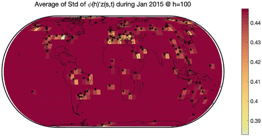
www.nature.com/scientificreports/
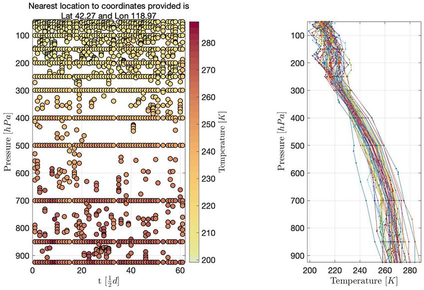
Figure 1. In the left panel, the vertical axis on the left represents pressure, and the vertical axis on the right
represents temperature. The horizontal axis represents time points, and data are collected every half day. In the
right panel, the vertical axis represents pressure, and the horizontal axis represents temperature. Data collected
at different times are represented by lines of different colors. All data are collected at the latitude 42.27 and
longitude 118.97 in January 2015.
given by B-spline basis functions. The spline coefficients, indexed in space and time, are modelled as spatiotem-
poral models on the sphere. In fact, we use an extension of the observation-minus-background approach, which
is common in atmospheric sciences17,18 and filter out large scale components.
The rest of the paper is organized as follows. “Datasets” section describes the RAOB dataset, and the ERA-
interim reanalysis data, which is used as the background. In “4D spatiotemporal statistical model” section, we
present the 4D spatio-temporal statistical model. “Model results” section reports the model results, and “Con-
clusion” section concludes.
Datasets
In this section, we introduce the data used for the estimation and validation of the model: the RAOB radiosonde
temperature vertical profiles which are used as the model response, and the European Centre for Medium-range
Weather Forecasts (ECMWF) ERA-interim reanalysis data, which are used as the background.
The universal rawinsonde observation program. In this paper, we use the RAOB dataset for January,
2015. This dataset is obtained from the database implemented by the Earth System Research Laboratory of the
National Oceanic and Atmospheric Administration (NOAA/ESRL, https://ruc.noaa.gov/raobs/).
We consider twice a day observations at 00:00 UTC and 12:00 UTC from the n = 200 worldwide launch
sites. Temperature data collected at the latitude 42.27 and longitude 118.97 in January 2015 is depicted in Fig. 1,
where the y-axis presents the barometric pressure levels.
A radiosonde is made by a set of instruments carried into the atmosphere by a weather balloon, measuring
various atmospheric parameters and transmitting them by radio to a ground receiver up to altitudes of approxi-
mately 30–35 km, depending on the balloon burst. The observations are processed and encoded for transmission
and efficient storage. While the radiosonde transmits an essentially continuous stream of temperature readings
back to the station (each 5–10 m of altitude, measured each 1–2 s), only a subset of this information is encoded
and transmitted.
ERA‑interim description. ERA-Interim is a global atmospheric reanalysis data provided by ECMWF. It
is based on assimilating global observations into a computational model which gives the best state estimate19.
We focus on 00:00 UTC and 12:00 UTC reanalysis which are described as instantaneous, though they represent
30 min averages and have a horizontal resolution of 0.75o, which is about 80 km depending on latitude. The
product comprises 60 vertical levels from the surface up to 0.1 hPa, and each level is populated by 241 × 480
pixels.
Scientific Reports | (2021) 11:18691 | https://doi.org/10.1038/s41598-021-98125-2 2
Vol:.(1234567890)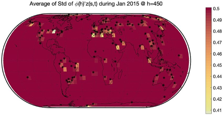
www.nature.com/scientificreports/
Figure 2. Example of a B-spline basis with 5 functions represented by 5 different colors.
4D spatiotemporal statistical model
In this section, we introduce a 4D spatiotemporal statistical model, which fits the functional data on the sphere.
Let yTEMP (s, h, t) be the atmospheric profile at site with coordinates s = (lat, lon) ∈ S2 and time t , observed at
altitude or barometric pressure h , where S2 is the sphere representing the Earth. The model is defined by the
following measurement and dynamics equations:
yTEMP (s, h, t) = xERA (s, h, t)βERA (h) + φ(h)′ z(s, t) + ǫ(s, h, t), (1)
z(s, t) = Gz(s, t − 1) + η(s, t). (2)
In this model, yTEMP (s, h, t) represents RAOB data and xERA (s, h, t) represents ERA-Interim reanalysis data.
Among (1), s represents different position of launching site on the two-dimensional plane of longitude and lati-
tude, h represents the third dimension of altitude or pressure, and t represents the fourth dimension of time. In
addition, φ(h)′ z(s, t) means the difference between RAOB data and ERA-Interim reanalysis data with altitude
h in position s at time t . To this end, this is a 4D model, which is relatively novel. This model is very different
from conventional 3D models in traditional literature. In the case study, we define h ∈ H = [50, 925] hPa ,
t = 1, . . . , 62. In the measurement equation, ǫ(s, h, t) is a Gaussian measurement error. The variance of ǫ(s, h, t)
is represented as σǫ2 (h). To this end, σǫ2 (h) needs to satisfy the following condition:
log σǫ2 (h) = φ(h)′ cǫ , (3)
where φ(h) is a set of p × 1 basis functions, and βERA (h) is modelled as:
βERA (h) = φ(h)′ cβ , (4)
where cβ is a p × 1 vector needed to be estimated. In Eq. (2), z(s, t) is a p-variate latent random variable with
Markovian dynamics ruled by the persistency matrix G. Therefore, G matrix is the correlation coefficient matrix
of latent random variable z(s,t) in time. In the dynamics equation, η(s; t) is a p dimensional Gaussian innovation
random field which is independent in time, with spatial covariance function:
Ŵ s, s′ ; θ = diag v1 ρ s, s′ ; θ1 , . . . , vp ρ s, s′ ; θp . (5)
In fuction (5), v = (v1 , . . . , vp )′ is the variance vector, and ρ s, s′ ; θj is a valid spatial correlation f unction20
on the sphere with range parameter θj from θ = (θ1 , . . . , θp )′ . In addition, “diag()” means the elements on the
diagonal of the matrix.
The O − B approach is generalized here by using the ERA-interim background as the unique covariate of
model, where O refers to observations and B refers to background21. In fact, the O − B approach is generalized
to O = βB + e, where e = ′ z + ǫ is capable to give a more detailed description of the bias structure. To model
the effect of the East–West atmospheric dynamics on the O − B error, the following simple anisotropic correla-
tion structure is used:
d s,s′ l −l ′
ρ s, s′ ; θ = exp − (θ(1) ) exp − | 1θ(2)1 | . (6)
In this paper, we use the B-spline system (B-spline) as φ(h) in the above model equation. Knots are the values
of where the pieces of polynomial meet, which are denoted and sorted into nondecreasing order. Figure 2 shows
Scientific Reports | (2021) 11:18691 | https://doi.org/10.1038/s41598-021-98125-2 3
Vol.:(0123456789)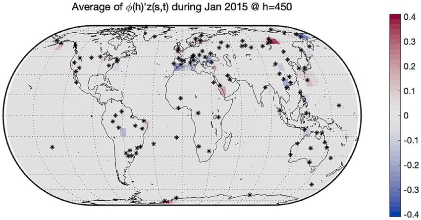
www.nature.com/scientificreports/
cβ Estimates Std. error t-statistic
Basis_1_@ERA 0.999 0.000 6709.991
Basis_2_@ERA 1.000 0.000 6045.506
Basis_3_@ERA 0.999 0.000 8770.185
Basis_4_@ERA 0.998 0.000 9224.893
Basis_5_@ERA 1.000 0.000 10,071.891
Basis_6_@ERA 0.999 0.000 10,766.577
Basis_7_@ERA 0.999 0.000 9800.519
Basis_8_@ERA 0.999 0.000 8499.463
Basis_9_@ERA 1.000 0.000 8200.708
Table 1. Result of cβ estimates.
cǫ Estimates Std. error t-statistic
Basis_1 1.444 0.015 93.849
Basis_2 1.137 0.026 44.112
Basis_3 0.519 0.021 24.539
Basis_4 0.024 0.025 0.972
Basis_5 0.499 0.029 17.490
Basis_6 0.519 0.024 21.602
Basis_7 0.004 0.024 0.165
Basis_8 0.790 0.028 28.027
Basis_9 0.400 0.022 18.005
Table 2. Result of cǫ estimates.
a B-spline curve with an order of 3 and knots of 3, with the vertical dashed line as the internal breakpoint that
defines the spline curve. Note that the sum of the B-spline basis function values at any point h is equal to 1.
Model results
We first estimated the model by Expectation–Maximization algorithm. Second, we analyzed the model estimation
results and verified the fitting goodness of our model based on cross-validation R 2 . Finally, based on the results
of spatial prediction, we analyzed the observation gaps by O − B approach.
Model estimation results. We choose Bspline to model Eqs. (1–2). As the accuracy of the data at high
altitude decreases, we set more internal breakpoints at high altitudes where the barometric pressure is below
300 hPa . Based on the empirical analysis, we set the parameter knots for estimating βERA (h) and σǫ2 (h) as
knots = [50, 150, 210, 290, 380, 510, 700, 925].
The estimated coefficient z(s, t) of the latent term φ(h)′ z(s, t) in Eq. (1) is p-variate latent Gaussian random
variable. Since the computation burden would be pretty high if too many knots are set, here the knots is as
knots = [50, 340, 925].
We implement a cubic spline here. Therefore, the number of basis functions for βERA (h), σǫ2 (h) and φ(h)′ z(s, t)
is 9, 9, 4 respectively. Tables 1 and 2 show the estimate results for cβ and cǫ.
We plot the βERA (h) and σǫ2 (h) estimates in Fig. 3. We can find that in the low-altitude layer with barometric
pressure higher than 400 hPa , the estimated value of βERA (h) is close to 1, and the variance σǫ2 (h) of the residuals
is pretty low. In the atmosphere where the barometric pressure is lower than 400 hPa , the variance σǫ2 (h) of the
residuals increases, and βERA (h) deviates from the value 1. Thus, our model captures the bias from high-level
RAOB temperature data, benefiting the accuracy of estimation of parameters.
Model fitting goodness. In this section, 30% sites are randomly selected as test set, and the remaining
70% sites are used for model estimation as training set. The real value and the predicted value from test set are
defined as y = (y1 , y2 , . . . , yn1 ) and y ∗ = (y∗1 , y∗2 , . . . , y∗n1 ) respectively, where n1 represents the number of
sites in the test set. By comparing the predicted value with the real value for the selected 30% sites, we obtain the
2 n1 n1 2
cross-validation R2 of the RAOB data model. Specifically,R2 = 1 − n1 k=1 (y ∗ −y) / k=1 (y − k=1 yk /n1 ) .
We show the fitting criteria R2 with respect to barometric pressure h, time t , and launching site s , respectively,
in Figs. 4 and 5. Note that, due to the continuous barometric pressure levels, we divide the pressure domain
Scientific Reports | (2021) 11:18691 | https://doi.org/10.1038/s41598-021-98125-2 4
Vol:.(1234567890)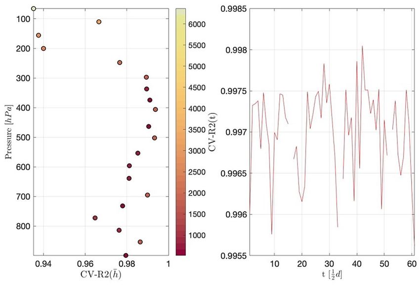
www.nature.com/scientificreports/

                                  Figure 3.  βERA (h) estimate and its 90%, 95%, 99% confidence bands (left), σǫ2 (h) estimate and its 90%, 95%,
                                  and 99% confidence bands (right). Among them, the outermost light red border on both sides represent 90%
                                  confidence bands, red border in the middle of both sides represent 95% confidence bands, and the innermost
                                  crimson border on both sides represent 99% confidence bands.

                                  Figure 4.  In the left panel, the horizontal axis represents cross-validation R 2 with respect to h and the vertical
                                  axis represents pressure. In the right panel, the horizontal axis represents different time and the vertical axis
                                  represents cross-validation R 2 with respect to t.

                                  [50, 925] hPa into 20 equally intervals, and calculate the cross-validation R2 within these intervals. Therefore, the
                                  color bar, of the left part of Fig. 4, represents the number of data in each interval.
                                      The left part of Fig. 4 shows that as the altitude increases, the cross-validation R 2 becomes smaller. In gen-
                                  eral, excluding the four upper-altitude intervals, the criteria R 2 higher than 0.96 is achieved, indicating the high
                                  accuracy of model prediction. The right part of Fig. 4 shows that R 2 fluctuates randomly over time. According

Scientific Reports |   (2021) 11:18691 |               https://doi.org/10.1038/s41598-021-98125-2                                                        5

                                                                                                                                                 Vol.:(0123456789)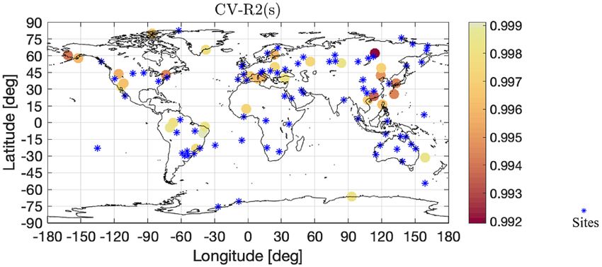
www.nature.com/scientificreports/
Figure 5. It shows Cross-validation R 2 with respect to sites s . The larger the value of Cross-validation R 2, the
lighter the color on the map. Sites used for model estimation are marked with blue stars. The values of Cross-
validation R 2 are relatively large. The software used to create the maps in the figure legend is Matlab 2018b, and
can be downloaded at https://www.mathworks.com/products/new_products/release2018b.html.
Figure 6. The average difference φ(h)′ z(s, t) between RAOB and ERA-Interim in January 2015 at 450 hPa. The
bigger the gap, the darker the color. All 200 sites are marked with black stars. The differences in areas where
there are sampling sites can be estimated well with color marked on the map. The differences in areas far away
from sampling sites cannot be estimated well with gray marked on the map. The software used to create the
maps in the figure legend is Matlab 2018b, and can be downloaded at https://www.mathworks.com/products/
new_products/release2018b.html.
to Fig. 5, we find that the accuracy of the prediction is higher in the densely site-located areas; otherwise the
accuracy of the prediction is lower.
Observation gap analysis. A typical use of the estimated model is to gather information on atmosphere
where no measurement are available. The average O − B profile and the average standard deviation profile are
given by
e(h) = �(h)z, (7)
σ e (h) = �(h)Var(z)�(h)′ , (8)
where z is the average of latent space–time variable z(s, t).
As mentioned in the introduction, the GAIA-CLIM project suggests to consider as observational gaps the
areas of the atmosphere where the uncertainty of spatial prediction is higher. Figure 6 shows the average estimates
of the difference φ(h)′ z(s, t) between the RAOB and ERA-Interim at pressure level 450 hPa . As it is expected,
the differences in areas where there are sampling sites can be estimated well with color marked on the map. To
visualize the changes of the average uncertainty of spatial prediction along different altitudes, we drew Figs. 7
and 8. These two Figures aim to show the value of σ e (h) with different h. Figures 7 and 8 depict the average of
Scientific Reports | (2021) 11:18691 | https://doi.org/10.1038/s41598-021-98125-2 6
Vol:.(1234567890)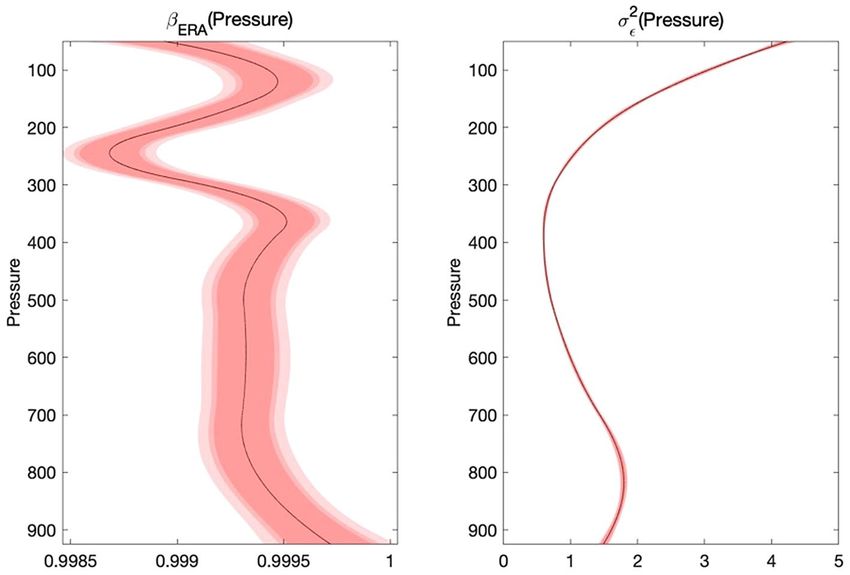
www.nature.com/scientificreports/
Figure 7. The average standard deviation of difference between RAOB and ERA-Interim in January 2015 at
450 hPa. All 200 sites are marked with black stars. The variance of differences in areas where there are sampling
sites are very small, while the variance of differences in areas far away from sampling sites are very large. The
software used to create the maps in the figure legend is Matlab 2018b, and can be downloaded at https://www.
mathworks.com/products/new_products/release2018b.html.
Figure 8. The average standard deviation of difference between RAOB and ERA-Interim in January 2015 at
100 hPa. All 200 sites are marked with black stars. The variance of differences in areas where there are sampling
sites are very small, while the variance of differences in areas far away from sampling sites are very large. The
software used to create the maps in the figure legend is Matlab 2018b, and can be downloaded at https://www.
mathworks.com/products/new_products/release2018b.html.
the standard deviations of the spatial predictions at barometric pressures 450 hPa and 100 hPa , respectively. We
found that, no matter what the altitude is, the variance of differences in areas where there are sampling sites are
very small, while the variance of differences in areas far away from sampling sites are very large. In this way,
we explore the underlying mechanism of how the uncertainty changing at various barometric pressure levels.
Conclusion
Meteorological data such as temperature data of the upper atmosphere is essential for accurate weather fore-
casting. In this paper, we propose a 4D spatiotemporal model that objectively measures the observation gap
of two types of temperature data (RAOB data and ERA-Interim reanalysis data). Based on the O − B method,
the observation gap is analyzed through the spatial prediction results. The estimated results of the model are of
significantly practical interpretation, and the model is meaningful in theory and practice.
From the theoretical point of view, we propose a 4D statistical model on the basis of traditional 3D model.
This model not only considers the traditional third dimension of time, longitude and latitude, but also the
dimension of altitude. Our model effectively characterizes the vertical profile of the radiosonde data through a
linear combination of random components and B-spline curves. We establish the model with these two kind of
temperature data from 200 launching sites worldwide in January 2015. The model shows a good model fitting-
ness by the criteria the cross-validation R 2.
From an application point of view, it can help climate scientists make effective inferences from ERA-Interim
reanalysis data to RAOB data. As mentioned before, ERA-Interim reanalysis data is widely available with low-
quality; RAOB data with high-quality but can offer a very limited spatial coverage. Through the method we
Scientific Reports | (2021) 11:18691 | https://doi.org/10.1038/s41598-021-98125-2 7
Vol.:(0123456789)www.nature.com/scientificreports/
proposed, we can obtain a huge amount of RAOB data with high-quality and can offer a very wide spatial cover-
age. We explored the underlying mechanism of how the temperature of atmospheric regions changing at different
barometric pressure levels, thus providing a meaningful reference for global climate prediction.
Received: 24 April 2021; Accepted: 3 September 2021
References
1. Upmanis, H. & Chen, D. Influence of geographical factors and meteorological variables on nocturnal urban-park temperature
differences—A case study of summer 1995 in Göteborg, Sweden. Clim. Res. 13(2), 125–139 (1999).
2. Lancaster, I. N. Relationships between altitude and temperature in Malawi. S. Afr. Geogr. J. 62(1), 89–97 (1980).
3. Piao, S. et al. Altitude and temperature dependence of change in the spring vegetation green-up date from 1982 to 2006 in the
Qinghai-Xizang Plateau. Agric. For. Meteorol. 151(12), 1599–1608 (2011).
4. Li, Y. & Ni, J. The characteristics of temperature variability with terrain, latitude and longitude in Sichuan-Chongqing Region. J.
Geogr. Sci. 22(2), 223–244 (2012).
5. Rattigan, K. & Hill, S. J. Relationship between temperature and flowering in almond: Effect of location. Aust. J. Exp. Agric. 27(6),
905–908 (1987).
6. Marion, G. M. et al. Open-top designs for manipulating field temperature in high-latitude ecosystems. Glob. Change Biol. 3(S1),
20–32 (1997).
7. Hammond, K. A., Szewczak, J. & Król, E. Effects of altitude and temperature on organ phenotypic plasticity along an altitudinal
gradient. J. Exp. Biol. 204(11), 1991–2000 (2001).
8. Rojas-Valverde, D., Ugalde-Ramírez, J. A., Sánchez-Ureña, B. & Gutiérrez-Vargas, R. Influence of altitude and environmental
temperature on muscle functional and mechanical activation after 30’time trial run. MHSalud 17(1), 19–33 (2020).
9. Li, B., Wang, Z., Jiang, Y. & Zhu, Z. Temperature control and crack prevention during construction in steep slope dams and stilling
basins in high-altitude areas. Adv. Mech. Eng. 10(1), 1687814017752480 (2018).
10. Merchant, C. J. et al. Uncertainty information in climate data records from earth observation. Earth Syst. Sci. Data 9, 511–527
(2017).
11. Lizundia-Loiola, J., Otón, G., Ramo, R. & Chuvieco, E. A spatio-temporal active-fire clustering approach for global burned area
mapping at 250 m from MODIS data. Remote Sen. Environ. 236, 111493 (2020).
12. Von Clarmann, T. et al. Overview: Estimating and reporting uncertainties in remotely sensed atmospheric composition and
temperature. Atmos. Meas. Tech. 13(8), 4393–4436 (2020).
13. Ignaccolo, R., Franco-Villoria, M. & Fassò, A. Modelling collocation uncertainty of 3D atmospheric profiles. Stoch. Environ. Res.
Risk Assess. 29(2), 417–429 (2015).
14. Wang, Y., Finazzi, F., & Fassò, A. D-STEM v2: A Software for Modelling Functional Spatio-Temporal Data. arXiv preprint arXiv:
2101.11370 (2021).
15. Giraldo, R., Delicado, P. & Mateu, J. Ordinary kriging for function-valued spatial data. Environ. Ecol. Stat. 18(3), 411–426 (2011).
16. Giraldo, R., Delicado Useros, P. F., & Mateu, J. Geostatistics for functional data: An ordinary kriging approach (2007).
17. Desroziers, G., Berre, L., Chapnik, B. & Poli, P. Diagnosis of observation, background and analysis-error statistics in observation
space. Q. J. R. Meteorol. Soc. 131, 3385–3396. https://doi.org/10.1256/qj.05.108 (2005).
18. Wang, Y., & Bai, Y. Estimating Observation Error Statistics Using a Robust Filter Method for Data Assimilation. In FSDM, 449–456
(2020).
19. Dee, D. P. et al. The ERA-Interim reanalysis: Configuration and performance of the data assimilation system. Quart. J. R. Meteorol.
Soc. 137, 553–597 (2011).
20. Porcu, E., Bevilacqua, M. & Genton, M. G. Spatio-temporal covariance and cross-covariance functions of the great circle distance
on a sphere. JASA. 11, 888–898 (2016).
21. Poli, P. et al. Pre-assimilation feedback on a Fundamental Climate Data Record of brightness temperatures from Special Sensor
Microwave Imagers: A step towards MIPs4Obs? ERA report series (2015).
Acknowledgements
This research is supported by National Natural Science Foundation of China (Grant No. 12001102) and “the
Fundamental Research Funds for the Central Universities” in University of International Business and Econom-
ics (No. 19QD22).
Author contributions
K.X. and Y.W. wrote the main manuscript text. All authors reviewed the manuscript.
Competing interests
The authors declare no competing interests.
Additional information
Correspondence and requests for materials should be addressed to K.X.
Reprints and permissions information is available at www.nature.com/reprints.
Publisher’s note Springer Nature remains neutral with regard to jurisdictional claims in published maps and
institutional affiliations.
Scientific Reports | (2021) 11:18691 | https://doi.org/10.1038/s41598-021-98125-2 8
Vol:.(1234567890)www.nature.com/scientificreports/
Open Access This article is licensed under a Creative Commons Attribution 4.0 International
License, which permits use, sharing, adaptation, distribution and reproduction in any medium or
format, as long as you give appropriate credit to the original author(s) and the source, provide a link to the
Creative Commons licence, and indicate if changes were made. The images or other third party material in this
article are included in the article’s Creative Commons licence, unless indicated otherwise in a credit line to the
material. If material is not included in the article’s Creative Commons licence and your intended use is not
permitted by statutory regulation or exceeds the permitted use, you will need to obtain permission directly from
the copyright holder. To view a copy of this licence, visit http://creativecommons.org/licenses/by/4.0/.
© The Author(s) 2021
Scientific Reports | (2021) 11:18691 | https://doi.org/10.1038/s41598-021-98125-2 9
Vol.:(0123456789)You can also read