An Enhanced Optical Flow Technique for Radar Nowcasting of Precipitation and Winds
←
→
Page content transcription
If your browser does not render page correctly, please read the page content below
DECEMBER 2017                                  BECHINI AND CHANDRASEKAR                                                                   2637

                      An Enhanced Optical Flow Technique for Radar Nowcasting of
                                       Precipitation and Winds

                                           RENZO BECHINI,a AND V. CHANDRASEKAR
                                               Colorado State University, Fort Collins, Colorado

                                    (Manuscript received 22 June 2017, in final form 15 September 2017)

                                                                  ABSTRACT

                  The atmospheric state evolution is an inherently highly complex three-dimensional problem that numerical
                weather prediction (NWP) models attempt to solve. Although NWP models are being successfully employed
                for medium- and long-range forecast, their short-duration forecast (or nowcast) capabilities are still limited
                because of model initialization challenges. On the lower end of the complexity scale, nowcasting by ex-
                trapolation of two-dimensional weather radar images has long been the most effective tool for nowcasting
                precipitation. Attempts are being made to take advantage of both approaches by blending extrapolation and
                numerical model forecasts. In this work a different approach is presented, relying on the additional Doppler
                radar wind information and a simplified modeling of basic physical processes. Instead of mixing the outputs of
                different forecasts as in blended approaches, the idea behind this study is to combine extrapolation and
                precipitation modeling in a new technique with a higher level of complexity with respect to conventional nowcasting
                methods, although still much simpler than NWP models. As a preliminary step, the Variational Doppler Radar
                Analysis System (VDRAS) is used to provide an initial analysis exploiting all the available dual-polarization and
                Doppler radar observations. The rainwater and wind fields are then advected using an optical flow technique that is
                subject to simplified physical interactions. As a result precipitation and wind nowcasting are obtained and are
                successively validated up to a 1-h lead time, showing potential improvement upon standard extrapolation.

1. Introduction                                                            forecast typically shows poorer performance with respect
                                                                           to methods based on the simple extrapolation of the ob-
   The description of the atmospheric state evolution is
                                                                           served reflectivity or related quantity (Germann and
inherently a three-dimensional problem involving sev-
                                                                           Zawadzki 2002; Hwang et al. 2015).
eral variables (e.g., for warm rain process: temperature,
                                                                             Extrapolation-based precipitation nowcasting ex-
humidity, pressure, winds, water vapor, cloud water,
                                                                           clusively relies on one variable (typically the radar
rainwater). However, nowcasting by radar is in general
                                                                           reflectivity) observed on a given surface, for example,
intended as the two-dimensional forecast of rainwater qr
                                                                           the conical scan surface. Nowcasting by extrapolation
(g kg21) in the near-surface layer. One possible option
                                                                           often makes use of optical flow techniques to estimate
for precipitation and wind nowcasting is through the use
                                                                           the motion vectors based on two or more previous
of numerical weather prediction (NWP) models on a
                                                                           observations. The motion vectors are then used to
limited domain, and considering a specific section of
                                                                           advect in time the most recent observations. Given the
the forecasted atmospheric state, that is, three variables
                                                                           huge difference in terms of complexity between the
(a precipitation-related quantity and the two wind com-
                                                                           model and the extrapolation approaches, the perfor-
ponents) on a single horizontal layer. While data assimi-
                                                                           mance attainable by adopting the latter technique
lation is contributing to improving the skill of NWP
                                                                           for precipitation nowcasting is somewhat surprising.
models at short lead times (Ballard et al. 2016), over
                                                                           The reason is that in general the advective compo-
a forecast range on the order of ;60 min the model
                                                                           nent of the storm evolution prevails over the more
                                                                           complex dynamical and microphysical interactions
  a
      Current affiliation: Arpa Piemonte, Turin, Italy.
                                                                           within the storm and with the surrounding environ-
                                                                           ment. Extrapolation-based methods provide good re-
  Corresponding author: Renzo Bechini, r.bechini@arpa.                     sults for very short-term forecasting (up to about
piemonte.it                                                                20 min), but their performance tends to quickly

DOI: 10.1175/JTECH-D-17-0110.1
Ó 2017 American Meteorological Society. For information regarding reuse of this content and general copyright information, consult the AMS Copyright
Policy (www.ametsoc.org/PUBSReuseLicenses).
                                                                                                      Unauthenticated | Downloaded 08/26/21 06:04 AM UTC
2638                 JOURNAL OF ATMOSPHERIC AND OCEANIC TECHNOLOGY                                                VOLUME 34

decrease as result of the absence of a representation            This work represents an attempt to model the in-
of the atmospheric physics, more specifically:                 terconnections between the rainwater and the low-level
                                                               wind evolution, relying on the independent estimation
d   There is a lack of source/sink terms: the most recent
                                                               of the motion vectors for the rainwater and for the
    observations are simply advected, assuming Lagrang-
                                                               components of the wind field (divergence and vorticity).
    ian persistence, irrespective of possible growth or
                                                               The proposed technique is applied over the Dallas–Fort
    decay affecting the storm evolution.
                                                               Worth (DFW), Texas, region, where measurements
d   The motion vectors are estimated from observations
                                                               from multiple radars (NEXRAD and X-band systems)
    typically confined over a portion of the radar domain.
                                                               are available within the DFW Urban Demonstration
    When the storms are advected in regions originally not
                                                               Network. The scanning strategy of the small X-band
    showing radar echoes, the motion vector estimates
                                                               radars is inherited from the Center for Collaborative
    may lose their representativeness.
                                                               Adaptive Sensing of the Atmosphere (CASA) project’s
   The different skill at increasing lead times of extrap-     distributed collaborative adaptive sensing concept
olation and NWP models led to the development of               (Junyent et al. 2010) and is intended to sample with high
blending techniques, with the aim to take advantage of         time resolution the lower atmosphere (1–3 km AGL).
both methods (Seed et al. 2013; Hwang et al. 2015). In           The paper is organized as follows. Section 2 illustrates
this work a different approach is presented to attempt to      the analysis method based on a four-dimensional vari-
improve the skill of standard extrapolation methods,           ational assimilation of radar observations, while section 3
including the additional Doppler radar wind observa-           describes the optical flow technique employed for es-
tions and a simplified representation of the convective        timating the motion vectors from a pair of consecutive
precipitation process.                                         analyses. The parametric model for precipitation and
   The use of a four-dimensional data assimilation system      wind nowcasting is discussed in section 4, and the achieved
has the potential to provide an accurate low-level wind        results for a representative case study are presented in
analysis. Unlike simpler multiple-Doppler techniques, the      section 5. Finally, the main findings are summarized and
adoption of a cloud-scale numerical model in the assimi-       discussed in section 6.
lation process ensures the physical consistency between
the wind and the rainwater fields over the assimilation
                                                               2. Analysis
time window. The availability of a reliable estimation of
the low-level wind field may help to compensate the               Four-dimensional data assimilation techniques have
previously mentioned limitations of standard extrapola-        been introduced during the last couple of decades in
tion methods. In particular, the divergence of the low-        global and regional models (Rabier et al. 2000; Rawlins
level winds provides useful indications about the location     et al. 2007; Tanguay et al. 2012) to provide a temporal
of convergence (negative divergence) regions near the          extension with respect to previous three-dimensional
surface, where intensification of an existing storm or a new   variational systems. In large-scale models, the four-
development is more likely. On the other hand, the             dimensional assimilation process is mainly intended as
downdraft inferred from the positive divergence regions,       an optimal filter, but for the convective scale it becomes
in conjunction with the rainwater content evolution, may       fundamental to retrieve the unobserved variables. In fact,
be used to attempt a simple representation of the outflow      while for the mesosynoptic scale the conventional mete-
that is relevant to the evolution of the wind field in the     orological observations (surface measurements and
lower level (Cotton et al. 2010).                              upper-air soundings) provide adequate resolution to
   ‘‘Mean winds’’ methods have also been used with some        represent the model variables, for the convective scale
success to predict the storm motion. These methods rely        only weather radars are able to collect observations with
on the empirical evidence that the motion of the storms        enough spatial and temporal resolution, although for a
correlates well with the average wind in the low to mid-       reduced set of variables. In addition, the variables ob-
troposphere. For example, Davies and Johns (1993) used         served by weather radar are not among the model vari-
the average wind in the lowest 0–6 km AGL. The rain-           ables but are generally related to the water content and
water motion vectors estimated using the past storm lo-        winds through appropriate observation operators.
cation can therefore be regarded as representative of some        The Variational Doppler Radar Analysis System
weighted average of the lower tropospheric winds. It           (VDRAS) is an advanced data assimilation system spe-
seems then consistent to attempt to exploit the low-level      cifically designed for ingesting Doppler weather radar
wind prediction to update the initial estimate of the rain-    observations at the convective scale (Sun and Crook 1997,
water motion vectors during the forecasting phase, as-         1998). The system has been installed at many sites around
suming that the upper level winds will evolve more slowly.     the world and is typically running using long-range

                                                                                    Unauthenticated | Downloaded 08/26/21 06:04 AM UTC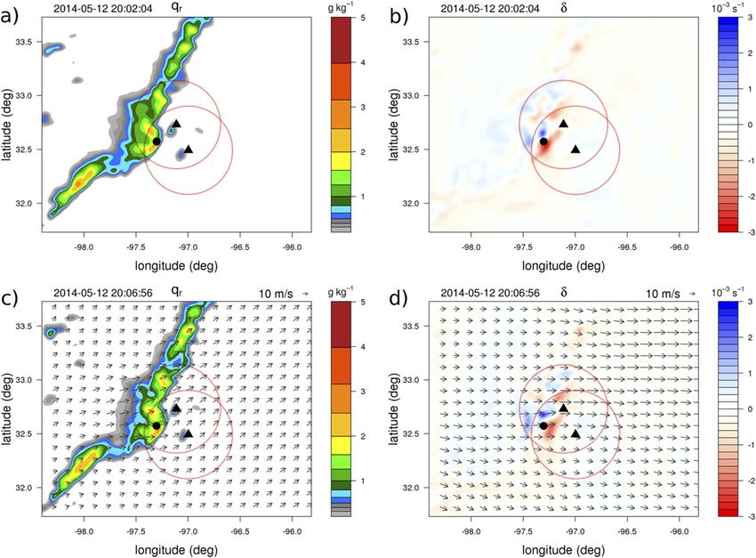
DECEMBER 2017                              BECHINI AND CHANDRASEKAR                                                                2639

FIG. 1. PPI from the Midlothian radar at 2039 UTC: (a) reflectivity, (b) hydrometeor classification, and (c) rainwater mixing ratio esti-
                                             mated from dual-polarization observations.

operational radar networks. The core four-dimensional                 Kdp and Zdr, and Kdp only, with coefficients as in Bringi
data assimilation scheme is based on a cloud-scale model              and Chandrasekar (2001).
and typically considers a 15–20-min time window for                     For assimilation in VDRAS, the radar observations of
the radar assimilation, with 1–3-km spatial resolution. The           radial Doppler velocity y obs
                                                                                                 r  and the estimates of qobs
                                                                                                                          r   in
analysis in this study is performed using VDRAS over                  the polar domain are first interpolated to Cartesian PPIs
the DFW region (Bechini et al. 2015).                                 with 500-m resolution. Figure 1 shows an example of a
                                                                      reflectivity PPI at 2.08 elevation from the Midlothian,
a. Radar data preprocessing                                           Texas, X-band radar, with hydrometeor classification
   The rainwater mixing ratio is conventionally derived               and the resulting qobs
                                                                                          r  estimation.
in VDRAS from reflectivity observations using a power-                b. Model setup
law relation obtained assuming a Marshall–Palmer
raindrop size distribution:                                             For the hailstorm event that occurred on 12 May 2014,
                                                                      the data from the S-band NEXRAD KFWS (DFW) ra-
                Zh 5 43:1 1 17:5 log10 (rqr ) ,                (1)    dar have been considered, in addition to the X-band ra-
                                                                      dars located in Arlington, Texas, and Midlothian. To
where Zh is the horizontal reflectivity (dBZ) and r is the            provide an initial condition (background) for the cost
air density. However, for X-band systems path attenua-                function minimization in VDRAS, a mesoscale analysis is
tion greatly affects the reliability of reflectivity-based            preliminarily performed to start the model simulation
estimates in heavy precipitation. Dual-polarization mea-              (cold start), based on surface observations (METARs)
surements allow for correcting path attenuation and for               and vertical sounding from a preliminary WRF Model
estimating the rain rate and the rainwater content with               simulation on a larger domain. The experiment started at
higher accuracy (Bringi and Chandrasekar 2001).                       1932UTC and then cycled every ;5 min, matching with
   In this work a blended algorithm is adopted that                   the NEXRAD volume update frequency (292 s) and us-
combines the available dual-polarization observations                 ing the previous forecast as background. This ensures the
in addition to Zh (namely, the differential reflectivity              availability of large-scale three-dimensional coverage for
Zdr and the specific differential phase shift Kdp) using              the analysis. The assimilation window is set to 3 min, al-
different relations, providing a rainwater estimate less              lowing for the inclusion of one S-band volume scan and
sensitive to drop size distribution (DSD) variations and              three to five low-level PPI scans from each X-band sys-
mostly unaffected by attenuation. The basis for apply-                tem. In previous VDRAS applications, assimilation
ing different relations is provided by a preliminary hy-              windows of about 15–20 min have been used, including
drometeor classification (Bechini and Chandrasekar                    several radar volume scans. The reference time for all the
2015) and according to predefined thresholds on the                   observations during the whole volume scan was the be-
dual-polarization variables (Cifelli et al. 2011). The                ginning of the first elevation scan, disregarding the time
relations used for the liquid water content (LWC)—                    differences between successive elevations. In the current
that is, the rainwater content mixing ratio scaled by air             setup, however, a short assimilation window is required to
density (LWC 5 rqr)—include functions of Zh and Zdr,                  consider the actual observation time of the individual

                                                                                             Unauthenticated | Downloaded 08/26/21 06:04 AM UTC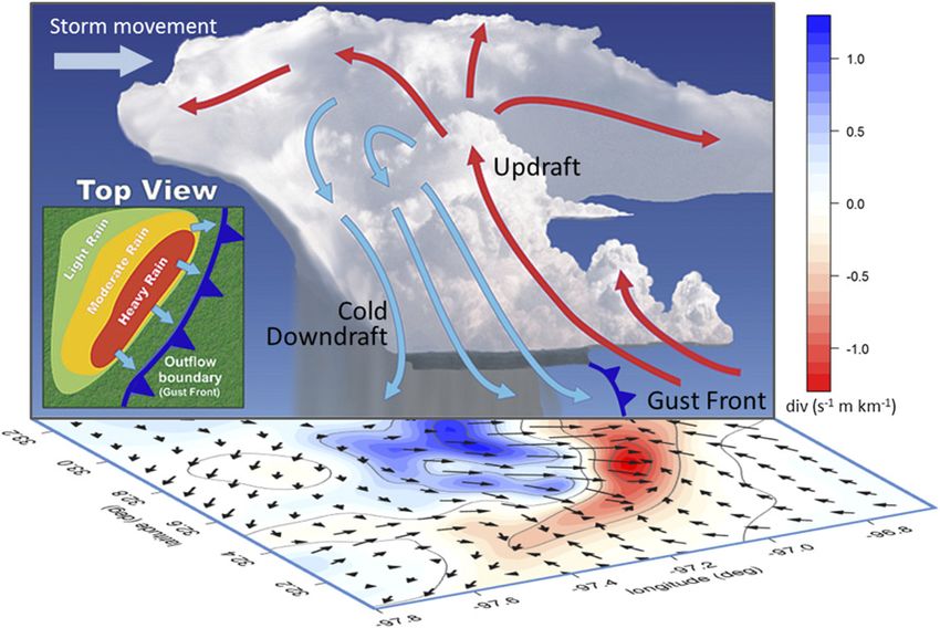
2640                JOURNAL OF ATMOSPHERIC AND OCEANIC TECHNOLOGY                                                       VOLUME 34

                    FIG. 2. VDRAS analysis at the 600-m vertical level of qr (colors) and winds at 1932 UTC from
                  the first cycle on the full model domain. Shown are the METAR surface observations (blue
                  wind barbs), the 40 km-range domain (red circles) of the two X-band radar (black triangles),
                  and the position of the NEXRAD KFWS radar (filled black circle).

PPIs within the NEXRAD volume scan, in order to deal              weather radar, important developments in optical flow
more consistently with the frequent low-level scans of the        techniques originate from lidar (Hamada et al. 2016;
X-band systems.                                                   Dérian et al. 2015) and satellite (Velden et al. 2005; Heas
   The model domain is 122 3 112 3 30 (nx, ny, nz, re-            and Memin 2008) applications. For weather radar, the
spectively) grid points, with a horizontal resolution of          most popular approaches are the block-based methods,
2 km, a vertical resolution of 400 m, and an integration          minimizing the sum of squared differences or maximizing
time step of 4 s. These parameters, in combination with           the normalized cross correlation (Rinehart and Garvey
the short assimilation window, allow for reducing the             1978; Chornoboy et al. 1994) or the variational methods
wall-clock time for the generation of a single analysis to        (Germann and Zawadzki 2002). Horn and Schunck
about 5 min, using 16 processors.                                 (1981) were the first to propose a variational method for
   In Fig. 2 the VDRAS analysis from the first (cold start)       optical flow estimation. In their seminal work, the basic
four-dimensional variational data assimilation (4D-Var)           optical flow constrain equation, frequently referred as the
cycle is shown on the full model domain. At this time, a          brightness constancy assumption, states that the apparent
squall line can be seen approaching from west-northwest           brightness I of moving objects remains constant over
within the DFW region covered by the X-band radars                time. This is expressed as
(red circles). The wind analysis during the following pe-
riod can then rely on multiple Doppler observations and                              dI              ›I
                                                                                        5 =I  u(x) 1 5 0 ,                     (2)
on several surface METAR measurements.                                               dt              ›t

                                                                  where u 5 (u, y) is the unknown motion vector field on
3. Motion vectors estimation
                                                                  the x 5 (x, y) plane. This equation cannot be solved
  Many techniques exist to estimate the motion of ob-             pointwise. In fact, because of the two unknowns, only
jects or surfaces from a sequence of ordered images.              the magnitude of the motion in the gradient direction
These techniques are generally referred to as optical flow        can be estimated. To solve this aperture problem, some
and can rely on different methods for the determination           additional constraints need to be introduced. Horn and
of the motion. In the atmospheric sciences, besides               Schunck proposed a variational method with global

                                                                                          Unauthenticated | Downloaded 08/26/21 06:04 AM UTC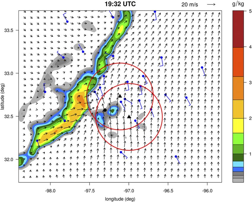
DECEMBER 2017                           BECHINI AND CHANDRASEKAR                                                          2641

smoothing to ensure filling in the motion estimate from          derive a reliable estimate ahead of the storm, exploiting
nearby gradient constraints. The variational problem is          the motion of the two small cells close to the two X-band
thus solved by minimizing an energy functional,                  radars (triangle symbol). The divergence (Figs. 3b,d)
                                                                 shows a westerly flow over most of the domain, also
     ð ð "                 2                        #
                                                                 ahead of the storm, with a small modulation across the
              ›I   ›I  ›I                 2       2
J5               u1 y1           1 a2 (j=uj 1 j=yj ) dx dy,      squall line. The motion fields of rainwater and the wind
              ›x   ›y  ›t
                                                                 components calculated from the VDRAS wind analysis
                                                          (3)    (divergence and vorticity) may show relevant differ-
                                                                 ences that are expected to bring useful complementary
where the parameter a is a regularization constant to            information to the forecast.
control the smoothness of the motion estimates. Larger
values of a lead to a smoother flow. The minimization of J       a. Semi-Lagrangian advection
can be achieved by solving the associated Euler–
                                                                    After the estimation of the motion vectors, the
Lagrange equations. The method relies on the proper
                                                                 advection of the rainwater and wind components can
estimation of the partial derivatives ›I/›x, ›I/›y, and ›I/›t.
                                                                 be accomplished using either forward or backward
If these cannot be correctly estimated because of highly
                                                                 schemes. Forward (in time) schemes foresee the distri-
nonlinear gradients or excessively large displacements of
                                                                 bution of the advected quantity among the neighboring
the precipitation patterns between successive images,
                                                                 grid points around the destination point (which in gen-
then the motion vectors cannot be correctly calculated.
                                                                 eral does not coincide with a grid point). If the flow is
To overcome the possible issue related to nonlinear
                                                                 divergent, however, this method may lead to ‘‘holes’’ in
gradients, the radar reflectivity (or logarithmic rainwater)
                                                                 the advected map. Another approach is to use backward
at a given vertical level is considered for the estimation of
                                                                 advection; that is, for a given grid point, the origin at the
the motion vectors. In fact, the rainfall rate (or liquid
                                                                 previous time step is found by following the flow back-
water) tends to show high peaks with exponential decay
                                                                 ward. This again will not coincide with a grid point, so
away from the precipitation core in convective pre-
                                                                 in this case interpolation is necessary (Germann and
cipitation. On the other hand, logarithmic quantities like
                                                                 Zawadzki 2002). Bilinear interpolation is often used for
reflectivity present a more linear decay. The second issue
                                                                 this purpose. However, in order to reduce the diffusion
may arise from either excessive physical displacements
                                                                 arising from the bilinear scheme, a bicubic interpolation
or a too high grid resolution. To overcome this possible
                                                                 is adopted here.
issue, the multiscale strategy approach of Meinhardt-
                                                                    The combination of the Lagrangian perspective and
Llopis et al. (2013) is adopted. In their method a pyra-
                                                                 the use of a regular grid Eulerian framework is known
midal structure provides a coarse-to-fine successive
                                                                 as the semi-Lagrangian scheme. This class of methods
refinement of the flow field. The input reflectivity images
                                                                 has the notable advantage of being particularly efficient,
are filtered and downsampled by a factor h using bicubic
                                                                 allowing for the use of large time steps.
interpolation. Starting at the coarsest scale, the optical
                                                                    The backward scheme is in general not mass conser-
flow equations are solved and every intermediate solution
                                                                 vative, although it may be considered nearly mass con-
is used as the initialization in the next scale. The h and the
                                                                 servative when the divergence of the flow field is
number of scales N are chosen based on the expected
                                                                 negligible. So, in order to ensure mass conservation, the
maximum storm motion, the grid resolution of the im-
                                                                 divergence component of the rainwater motion vectors
ages, and the time lag between two successive images, in
                                                                 field needs to be removed, or at least severely damped.
order to keep the motion to be detected small at the
                                                                 This is accomplished by relying on a technique widely
coarsest scale. For the case discussed in section 5, the
                                                                 used in fluid dynamics simulations (Stam 1999). Ac-
values h 5 0.5 and N 5 4 are used.
                                                                 cording to Helmholtz’s theorem, the wind vector field
   Figure 3 shows an example of motion vector estima-
                                                                 can be decomposed into an irrotational component
tion for the case study discussed in section 5, for the
                                                                 and a nondivergent component. For a horizontal wind
rainwater (Figs. 3a,c) and the divergence field obtained
                                                                 vector V, the vertical vorticity j and divergence d are
from the VDRAS wind analysis (Figs. 3b,d).The motion
                                                                 defined as
vectors for the rainwater show a dominant westerly
component on the squall line near the KFWS radar                                     ›y ›u                    ›u ›y
(moving eastward), while a southwesterly flow is esti-              j5k  =3V5         2 ,       d5=  V5       1 .         (4)
                                                                                     ›x ›y                    ›x ›y
mated ahead of the storm. This is in fair agreement with
the VDARS wind retrieval in the low levels (Fig. 2). In          The wind field can then be expressed in terms of the
this specific case, the optical flow method is able to           streamfunction c and velocity potential x:

                                                                                     Unauthenticated | Downloaded 08/26/21 06:04 AM UTC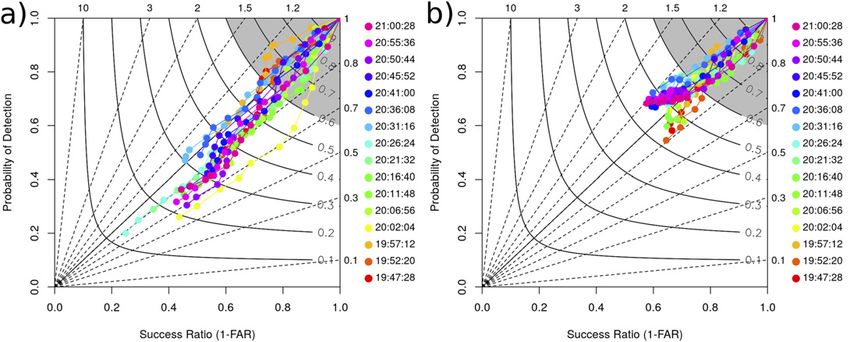
2642                  JOURNAL OF ATMOSPHERIC AND OCEANIC TECHNOLOGY                                                            VOLUME 34

              FIG. 3. Example of motion vector estimations. (a),(c) Rainwater analysis at 600-m height for two successive time
           steps (2002 and 2006 UTC). Based on the optical flow solution on this pair of images, the motion vectors in (c) are
           estimated. (b),(d) Corresponding motion vector estimations for the divergence fields at the same vertical level as in
           (a),(c). Only one vector every six grid points is plotted for clarity.

               V 5 Vc 1 Vx 5 =x 1 k 3 =c:                       (5)    unphysical visual deformations (excessive stretching/
                                                                       shrinking).
From Eq. (4) and taking the vertical component of the                  b. Image registration
curl and the divergence of Eq. (5), the Poisson equations
for j and d are obtained:                                                 As described in the next section, the parametric model
                                                                       relies on the analyses at two vertical levels for the esti-
                      =2 c 5 j, =2 x 5 d.                       (6)    mation of the rainwater content gradient. The vertical
                                                                       gradient is used to estimate the contribution to the
The divergent component of the motion vectors can                      rainwater in the lowest level by vertical advection.
then be subtracted in three steps:                                     However, possible tilting of the storm may affect this
                                                                       estimate by introducing artifact gradients. In fact, the
d   calculate divergence from the motion vector field
                                                                       two-dimensional model does not resolve the vertical
d   solve for the velocity potential x, given that =2x 5 d,
                                                                       wind shear, so the high-level rainwater needs to be
    using a iterative successive overrelaxation (SOR)
                                                                       aligned with the low-level field to compensate for the
    technique
                                                                       eventual tilting. In addition, depending on the scanning
d   subtract =x from the original motion vector field
                                                                       strategy and the analysis method, an apparent additional
  This procedure is especially important when the                      tilting may be introduced by the delayed radar scanning
motion vector field is mixed with the low-level                        of the higher elevations. Correction of the apparent
wind field during the forecast, as described later in                  misalignment can be performed through image regis-
section 4c. In fact the low-level wind field generally                 tration. Optical flow may also be used for this purpose,
has a quite relevant divergence component, which                       so the Horn–Schunck technique described in section 3 is
would severely impact the stability of the rainwater                   also applied to determine the appropriate deformation
advection in terms of mass conservation, causing                       (motion vectors) to align the upper-level rainwater field

                                                                                               Unauthenticated | Downloaded 08/26/21 06:04 AM UTC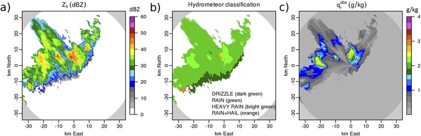
DECEMBER 2017                          BECHINI AND CHANDRASEKAR                                                         2643

to the lower-level rainwater field. In this preliminary        to reflectivity (rainwater) is here extended to the wind
evaluation of the method, the same optical flow pa-            components, and simple relations governing the rain
rameters used for the motion vector estimation of the          growth and decay are defined and heuristically tuned
rainwater and wind components are adopted, specifi-            through a set of adaptive parameters.
cally the regularization parameter a 5 80. This large             In an observational environment such as the DFW test
value of a (smooth displacement) may lead to an over-          bed, the architecture of the weather radar network
estimation of the vertical gradients in some cases, al-        provides the best coverage in the atmospheric layer
though the overall impact on the quality of the forecast       closer to the surface. From this perspective, the aim of
appears limited. Further investigation will be devoted to      the proposed approach is to extract the most valuable
assessing the impact of tilting in different conditions and    information content from the available observations. In
sensitivity to the optical flow settings.                      addition to the rainwater content, the analysis and
                                                               nowcast of the wind field near the surface have a special
4. Parametric model for nowcasting                             relevance of their own for the potential impact on hu-
                                                               man activities and infrastructures. A suitable represen-
   If the two basic assumptions for the optical flow—that      tation of the dynamics taking place in the lowest layer is
is, the stationarity of the motion vectors and the lack of a   also important for the tight relation with the storm
source term—are removed, then Eq. (2) becomes                  evolution.
                                                                  The basic steps of the parametric model are described
            dqr                  ›q
                5 =qr  u(t, x) 1 r 5 S(t, x).          (7)    in detail in the following subsections. The divergence
             dt                   ›t
                                                               and vorticity are initially calculated from the low-level
   If the level of brightness is not constant, then the        wind analysis. Considering a pair of observational time
motion estimate can be biased. To cope with this limi-         frames, typically lag-0 (time t0) and lag-1 (time t0 2 1),
tation, methods like the integrated continuity equation        the optical flow technique is applied independently to qr,
(ICE) have been developed and applied to satellite             d, and j, obtaining the motion vectors Uqr, Ud, and Uj,
imagery (Fitzpatrick 1988; Corpetti et al. 2002; Heas          respectively. The divergence and vorticity are advected
et al. 2007). Other attempts have also been made to            to the next time step using the respective motion vec-
develop methods including brightness variation caused          tors, while before applying advection to qr , its local
by time-dependent physical models (Haussecker and              rate of change at the two vertical levels is estimated
Fleet 2001), although these were mainly limited to rel-        (section 4a).
atively simple applications, such as changing illumina-
                                                               a. Growth and decay parameterization
tion or thermal diffusion in infrared images.
   The approach adopted here is based on a separate              The parameterization of the growth and decay local
treatment of the optical flow derived from Eq. (2) and         rate of change is realized according to the following
the local rate of change of the rainwater content and          equations:
winds. The proposed model relies on two consecutive
analyses from two vertical levels of the VDRAS assim-                      ›qr ›qr
                                                                               5    (w 1 Vt ) 1 p0 w,      and            (8)
ilation system:                                                             ›t   ›z
                                                                            Vt 5 5:40 q0:125
                                                                                       r     ,                            (9)
d   600 m MSL (rainwater and winds)
d   3400 m MSL (rainwater).
                                                               where Vt is the terminal fall velocity of raindrops (Sun
   The choice of the specific levels is dictated by the need   and Crook 1997), p0 is the condensation parameter
to have a sufficient vertical spacing inside the liquid        (Table 1), and w is the vertical velocity of air obtained
phase layer to calculate a reliable rainwater gradient         from the divergence in the hypothesis of mass conser-
(section 4a). While the VDRAS analysis provides the            vation. Since the divergence at the near-surface level
full set of atmospheric variables, only the radar ob-          (600 m) is being considered, assuming w 5 0 below this
servable fields (rainwater and winds) are considered in        level and zero divergence at the upper level (3400 m), a
this approach. The idea is to constrain the observations       positive (negative) divergence corresponds to negative
(analyses) using a simplified physical model with adap-        (positive) vertical velocity in this atmospheric layer.
tive parameters. It is argued that while the deficient         Equation (8) is basically the continuity equation for
physical description will inherently limit the validity of     precipitation originally derived by Kessler (1995). The
the forecast for large lead times, the adaptiveness of the     first term on the right represents the sedimentation
model may help to improve the very short-term forecast         (vertical advection) of rainwater, and the second term
(0–60 min). The traditional use of extrapolation applied       represents growth by condensation. Since cloud water qc

                                                                                   Unauthenticated | Downloaded 08/26/21 06:04 AM UTC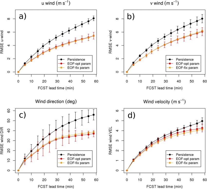
2644                        JOURNAL OF ATMOSPHERIC AND OCEANIC TECHNOLOGY                                                      VOLUME 34

 TABLE 1. Synthetic description of the parameters in the model.                The role of the lagged vertical velocity is therefore to
                                                                            heuristically contemplate the possible spatial displace-
Parameter                                          Description
                                                                            ment. After all, although the storm evolution is greatly
   p0                                Condensation
                                                                            dependent on the environmental shear profile (Rotunno
   p1                                Evaporation
   p2                                Vertical velocity lag                  et al. 1988), it is believed that the relative position
   p3                                Outflow divergence                     and propagation of the near-surface convergence with
   p4                                Forward–backward outflow factor        respect to the precipitation core has the potential to
   p5                                Mix-winds weight factor                provide valuable information to improve the very short-
                                                                            term prediction of the overall system motion and
                                                                            morphology.
                                                                               Rainwater vertical advection is applied only when
is not considered in this model, the microphysical con-
                                                                            there is a positive qr flux downward [Eq. (12)] in the
tributions to precipitation as a result of autoconversion
                                                                            current setting. Equation (12) may actually be applied
of cloud to rain and the accretion of cloud water by
                                                                            irrespective of the gradient and vertical velocity signs,
existing rain are not accounted for. In addition to sedi-
mentation and condensation, evaporation needs to be                         although this may imply negative qr values. Negative qr
represented in the model to ensure a precipitation bal-                     can be dealt with and provide a way to inhibit new
                                                                            convection in regions where persistent downdrafts have
ance. Following Kessler (1995) the depletion of rain by
                                                                            occurred. However, some preliminary tests showed that
evaporation can be represented as
                                                                            the adopted solution, exploiting the evaporation term to
                            ›qr                                             balance the overall rainwater budget, performed better.
                                5 p1 qc qr0:65 ,                     (10)      The coefficients p0 (condensation), p1 (evaporation),
                             ›t
                                                                            and p2 (lagged vertical velocity) are part of the param-
where p1 is the evaporation parameter (Table 1), and                        eters set to be determined adaptively through the opti-
with a strong approximation qc has to be assumed con-                       mization described below in section 4d.
stant (51) for being not represented in this context. For
practical implementation, since only two vertical levels                    b. Outflow parameterization
are considered, the parametric equations given above                           A downdraft generally develops within a thunder-
are applied to the upper (superscript 1) and lower (su-                     storm when precipitation falls through an unsaturated
perscript 0) levels:                                                        layer and evaporation starts cooling the air. The com-
                                                                            bined effect of precipitation loading (drag of liquid
     (qr )1t11 5 (qr )1t 1 p0 Lp2 wt dt;      Lp2 wt 5 wt2p ,        (11)   water) and evaporative cooling can lead to the forma-
                                                                 2

                                                                            tion of a cold pool, which is associated with damaging
                             (qr )1t 2 (qr )0t
    (qr )0t11 5 (qr )0t 1                      (w 1 Vt ) dt;                winds at the surface. In fact the downdraft approaching
                                     Dz
                                                                            the surface causes a divergent flow and a gust front
        (qr )1t . (qr )0t     and (w 1 Vt ) , 0, and                 (12)
                                                                            (outflow boundary) propagates, separating the cooler
          0,1
     (qr )t11 5 (qr )t0,1 1 p1 q0:65
                                r    dt ,                            (13)   air below the storm core from the environmental
                                                                            warmer air (Cotton et al. 2010). The speed of the ad-
where t and t 1 1 indicate the current and next time step,                  vancing gust front relative to the ambient flow is found
respectively; and dt is the forecast time interval. In Eq. (11)             to be close to the speed of a density current and can be
L denotes the lag operator; that is, Lp2 means lagging w by a               expressed in terms of the density difference between
period p2 (vertical velocity lag parameter). The lagged field               the surrounding air and the denser air within the cold
is obtained by advecting backward or forward in time the                    pool (Wakimoto 1982). However, in this context the
divergence (vertical velocity) using the estimated motion                   lack of any information about density (or pressure)
vectors. This is a necessary and important feature of the                   prompts an attempt to represent the flow associated
model to compensate for the lack of three-dimensionality,                   with the cold pool in terms of the vertical velocity and
in particular for squall lines with surface-based cold pools.               the evaporative cooling [Eq. (10)]. Because of the
In fact the regions of strong convergence near the surface,                 nonuniform surface winds and the three-dimensional
often associated with a gust front (Fig. 4), may move sig-                  flow organization, in particular the presence of a rear
nificantly away (often downwind) from the main storm                        inflow jet in squall lines causing cold air to be drawn in
core. This may result in a tilted warm inflow current turning               on the rear side of the storm (Cotton et al. 2010),
into the updraft. In this case the storm enhancement or new                 the divergent flow on the two-dimensional plane near
cell development will take place downwind with respect to                   the surface is in general not symmetric. To mimic this
the observed low-level convergence.                                         near-surface two-dimensional structure of the flow

                                                                                                 Unauthenticated | Downloaded 08/26/21 06:04 AM UTC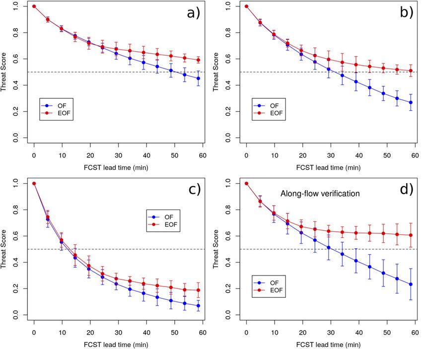
DECEMBER 2017                              BECHINI AND CHANDRASEKAR                                                              2645

                    FIG. 4. Idealized diagram of a squall-line vertical structure showing updrafts, downdrafts, and
                  a gust front. Precipitation forming in the tilted updraft falls into the downdraft. Beneath the
                  cloud, the denser cool air of the downdraft spreads out along the ground. On the leading edge of
                  the outflowing downdraft, a gust front may form, forcing the moist surface air to flow up into the
                  cloud. In the lower horizontal plane oriented perpendicular to the diagram, a real VDRAS
                  wind analysis from the case study discussed in section 5 (2021 UTC) is displayed with di-
                  vergence (color). The diagram and the horizontal analysis are subjectively matched with the
                  purpose of illustrating the relation between the low-level wind and the storm vertical devel-
                  opment. From the retrieved wind field, the average storm motion has been subtracted in order
                  to show the storm-relative winds. The diagram is adapted from the National Weather Service
                  Online Weather School (http://www.weather.gov/jetstream/tstrmtypes).

originating in downdraft regions, a term defining the                                    Uout 5 =x;      =2 x 5 d,                (15)
outflow strength is first introduced:
                                                                    where x is the velocity potential and the Dirichlet
             DIVout 5 p3 (w 1 Vt ) dE dt;                           boundary condition (null velocity on the boundary) is
                 dE 5 [(qr )0t11 ]0:65 2 [(qr )0t ]0:65 ,   (14)    assumed.
                                                                       The combination of the mean wind and the rear inflow
                 dE . 0 and (w 1 Vt ) , 0
                                                                    with the outflow causes the circulation within the cold
where p3 represents the outflow divergence parameter                pool to divert from the symmetric pattern arising from
(Table 1), and dE is the incremental rainwater mass loss            the SOR retrieval. In practice over time the cold pool
owing to evaporation between time steps t and t 1 1.                tends to elongate in the direction of the mean wind
Equation (14) is based on the knowledge that the out-               Corfidi (2003), with segments of the gust front oriented
flow produced at the surface is the consequence of both             parallel to the mean wind remaining quasi stationary,
the negative vertical velocity (producing divergence)               while segments perpendicular to the mean wind move
and cooling resulting from evaporation (producing a                 faster downwind. This behavior can be portrayed con-
spreading density current). The initial wind analysis al-           sidering the angle u between the unit vector representing
ready implicitly includes the outflow term, while for the           the motion of the wind field divergence (indicative of the
next predicted time steps the evolution of both the                 gust front propagation) and the irrotational flow vector
downdraft velocity and the rainwater mass needs to be               associated with the outflow [Eq. (15)]. A damp/
considered.                                                         strengthen factor is defined based on the dot product
   From the divergence term associated with the down-               between these two vectors as
draft [Eq. (14)], the corresponding irrotational flow                                    d 5 0:5 [p4 cos(u) 1 1]                  (16)
(Uout) is estimated using an SOR technique and recall-
ing Eqs. (5) and (6):                                               and applied to the outflow vector:

                                                                                            Unauthenticated | Downloaded 08/26/21 06:04 AM UTC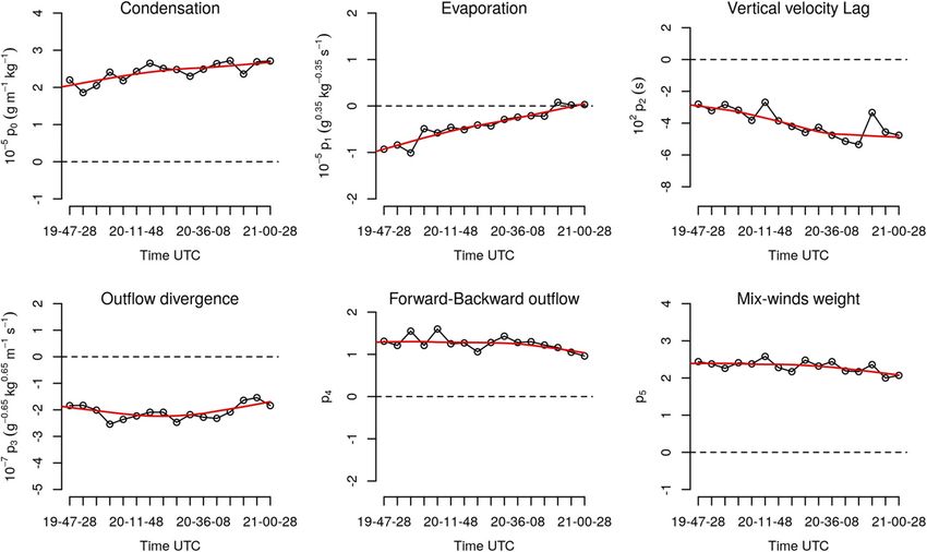
2646                   JOURNAL OF ATMOSPHERIC AND OCEANIC TECHNOLOGY                                                           VOLUME 34

  FIG. 5. Qualitative illustration of the flow representation within the cold pool on an arbitrary x–y plane. Shown are the intensity of the
divergence (gray shading), the storm-relative wind in the cold pool (black arrow), the direction of the divergence motion (red arrows), and
the outflow boundary (solid contour). (a) Backward (p4 5 21), (b) symmetric (p4 5 0), and (c) forward (p4 5 11) propagation.

                        V0out 5 d  Uout .                     (17)              and 3400m), compensating for possible real
                                                                                 (wind shear) or apparent (interscan delays)
When the forward–backward outflow factor parameter                               tilting of the storm; and
p4 is null ( p4 5 0), the flow is unaffected except for a 0.5               (ii) the intensity of the outflow, and the relative flow
scaling factor (Fig. 5b), while values of p4 , 0 and p4 . 0 are                  vectors, is estimated from the rainwater and
associated with backward and forward propagation, re-                            divergence at time t0 according to Eq. (14) (blue
spectively (Figs. 5a,c, respectively). The resulting flow                        blocks in the flow diagram).
V0out is finally added to the low-level wind field:                    2)   Optical flow estimation of the motion vectors is per-
                                                                            formed separately for the three fields: qr, and the two
                        U0 5 U 1 V0out .                       (18)         derived components of the wind field, that is, d and j.
                                                                       3)   Growth/decay terms are applied to the qr fields
                                                                            (lower and upper levels) according to Eqs. (11)–(13).
                                                                       4)   The fields qr, d, and j at t0 are advected to time step
c. Wind advection and mixing with rainwater motion
                                                                            t0 1 1 using the respective motion vectors (point 2),
   vectors
                                                                            relying on a backward advection scheme with bicubic
  Vorticity and divergence are calculated from Eq. (18)                     interpolation.
and advected using the respective motion vector esti-                  5)   From the updated qr and d at time t0 1 1, the new
mates. The wind field at time step t 1 1 (U0t11 ) is then                   intensity of the outflow and relative flow vectors is
calculated applying the SOR technique from the di-                          also estimated.
vergence and vorticity components, relying on the cur-                 6)   The advected d and j are combined with the outflow
rent time wind field (U0t ) as the first guess. The updated                 from point 1(ii) (which is also advected using the
low-level wind field is also used to adjust the rainwater                   motion vectors Ud) to retrieve the updated low-level
motion vectors, based on the previously discussed as-                       wind field at time step t0 1 1.
sumption that the storm motion is influenced by the                    7)   The updated low-level wind field is mixed with the qr
mean wind in the low to medium troposphere:                                 motion vectors at time t0 to provide new displacement
                                                                            vectors to advect qr forward from t0 1 1 to t0 1 2.
              Uqr 5 ( p5  U0 1 Uqr )=( p5 1 1) .              (19)
                                                                         For the successive time steps, points 3–7 are cyclically
                                                                       repeated, incrementing the time indexes. The time step
The flow-related coefficients p3, p4, and p5 complete the
                                                                       used in the forecast is the same as the time interval be-
set of six parameters (Table 1) that need to be determined.
                                                                       tween the pair of initial observations t0 and t0 2 1 (292 s).
  The general procedure is represented by the flow di-
                                                                       Experiments using shorter time steps for the forecast
agram in Fig. 6 and summarized in the following points:
                                                                       resulted in small differences.
1) The analysis (rainwater and wind) at the current (t0)
                                                                       d. Optimization of the model parameters
   and previous (t0 2 1) time steps are considered as
   input for the model:                                                 To find the optimal set of parameters, the Nelder–
    (i) image registration is applied in order to align the            Mead (NM) downhill simplex method [Nelder and
        rainwater fields at the two vertical levels (600               Mead (1965)] is adopted. The NM method belongs to

                                                                                                Unauthenticated | Downloaded 08/26/21 06:04 AM UTC
DECEMBER 2017 BECHINI AND CHANDRASEKAR 2647
FIG. 6. Schematic flow diagram of the nowcasting model. The growth/decay process includes sedimentation, condensation, and
evaporation (section 4a). The colors indicate observations/analysis (green background), the motion vectors (light green), the forecast
fields (orange), and the outflow modeling (dark blue). The orange arrows represent the wind mixing (section 4c). Superscripts 0 and 1 in
the analysis fields refer to the lower (600 m) and upper (3400 m) levels, respectively.
the class of direct search methods and is suitable global optimization algorithm, although in practice it
for multidimensional unconstrained optimization. The tends to work reasonably well for problems that do not
simple grounding idea and ease of implementation have many local minima. The objective function to
makes it a very popular method, used in a wide range of minimize in the current application is defined by the
scientific applications. The NM method is not a true following sum of root-mean-square errors:
D E0:5 D E0:5 D E0:5
fcst 2
r 2 qr )
(qobs (uobs 2 ufcst )2 (yobs 2 yfcst )2
f5 1 1
sqr su sy , (20)
sqr 5 0:2 g kg21 ; su 5 3:0 m s21 ; sy 5 3:0 m s21
where the average is calculated over the space–time to 158 min (12 time steps with dt 5 292 s) is started,
validation domain. The normalization factors in the using the current and the lag-1 fields for the optical flow
denominator are assumed constant. The spatial domain estimation. The forecasted qr and low-level winds U are
is a subdomain of the whole model domain (Fig. 8), to compared with the corresponding analyses for the esti-
avoid boundary effects, while the temporal domain ex- mation of the function f in the iterative optimization
tends from the analysis time until a given forecast lead procedure [Eq. (20)]. In the current implementation, all
time (e.g., 60 min). the parameters in the model (Table 1) are scaled during
the forecast by a factor of 1 (forecast 1 0 min) linearly
decreasing with lead time until zero (forecast 1
5. Results
120 min). In fact, since the model greatly relies on ex-
Considering the period between 1947 and 2100 trapolation (qr and winds) and the domain is limited
UTC 12 May 2014, a total of 16 analyses (one every (both the spatial domain and the variable space), the
292 s) are available. For each analysis a forecast up simple physical relations adopted [Eqs. (11)–(19)] will
Unauthenticated | Downloaded 08/26/21 06:04 AM UTC2648 JOURNAL OF ATMOSPHERIC AND OCEANIC TECHNOLOGY VOLUME 34
FIG. 7. Parameters obtained after NM optimization over 58-min forecasts between 1947 and 2100 UTC. A spline fit is superimposed (red)
to highlight the trend of the parameters with time.
inherently lose their adequacy during the forecast. The negative values) and trial and error forecast runs with
decreasing scaling factor is then adopted to give more varying configurations. The adopted initial set of values
confidence to the physical relations during the first is as follows: p0 5 12.0 3 1025, p1 5 20.5 3 1025,
stages of the forecast while trying to keep the perfor- p2 5 2600 s, p3 5 21.5 3 1027, p4 5 10.8, and p5 5 12.0.
mance robust for longer lead times. During the optimization, a 58-min forecast is run itera-
The validation is performed on the domain (repre- tively until convergence is reached. On average a single
sented by the rectangle in Fig. 8, 89 3 94 grid points), optimization loop took about 18 iterations and 39 func-
with a 2-km grid resolution. The results of the current tion evaluations. The resulting parameters are plotted
method are compared with the simple Horn–Schunck in Fig. 7 for every independent forecast. It can be seen
optical flow method described in section 3, based on qr that, although the 16 optimizations at successive times
motion vectors (called OF). are performed independently,1 the resulting parameters
For each of the 16 analyses in the study period, the are substantially stationary or smoothly changing.
Nelder–Mead optimization is performed to determine The parameter showing the most significant relative
the optimal set of model parameters. The optimization is variation is p1 (evaporation), passing from about 21.0 3
performed without constraints, but the choice of the 1025 at 1947 UTC to ;0 around 2050 UTC. As discussed
initial value of the parameters has an impact on the re- further later in this section, the evaporation term con-
sult, since Nelder–Mead is not a true global optimization tributes little or nothing to the skill of the forecast when
algorithm and it may converge to different local minima evaluated using the threat score, but it is useful for
depending on the initial setting. One way to overcome
this limitation would be to perform an outer loop uti-
lizing many initial simplicities in order to find the most
1
suitable part of the parameter space with which to start. However, the initial analyses are not completely independent.
In this preliminary evaluation, the initial parameters are In fact, for a given analysis time the VDRAS assimilation relies on
the background forecast from the previous cycle. This contributes
set to ‘‘reasonable’’ values based on the physical to guaranteeing physical consistency among successive analyses,
meaning of the processes involved (p0 and p5 are ex- and it can also reflect in the smooth evolution of the parameters
pected to be positive, while p1, p2, and p3 should assume resulting from the optimization.
Unauthenticated | Downloaded 08/26/21 06:04 AM UTCDECEMBER 2017 BECHINI AND CHANDRASEKAR 2649
FIG. 8. (left) Analysis and (right) corresponding forecasts every ;15 min of rainwater and low-level winds
starting at 2026 UTC. The solid contours represent the 0.5 (blue) and 20.5 s21 m km21 (black) divergence levels.
The domains of the X-band radars (red circles) and the validation area (rectangle) are marked. The color palette for
reflectivity (dBZ) is defined assuming a Z(qr) relation as in Sun and Crook (1997).
Unauthenticated | Downloaded 08/26/21 06:04 AM UTC2650 JOURNAL OF ATMOSPHERIC AND OCEANIC TECHNOLOGY VOLUME 34
FIG. 9. (left) Analysis between 2026 and 2124 UTC, (center) corresponding forecasts every ;20 min using standard OF, and (right)
parametric model forecast (EOF). The color palette is as in Fig. 8. For ease of comparison, the curved black line in the bottom row marks
the approximate position of the storm frontal line from the analysis.
maintaining the average rainwater level close to the images, a coarse grid with 0.58 latitude/longitude spacing
observations. is superimposed with letter/number coordinates in red
As an example, Fig. 8 shows the parametric model to facilitate the comparison. The forecast for successive
forecast starting at 2026 UTC, denoted enhanced optical lead times are displayed in the right column, while
flow (EOF). In this and the following analysis/forecast the left column reports the corresponding analysis. In
Unauthenticated | Downloaded 08/26/21 06:04 AM UTCDECEMBER 2017 BECHINI AND CHANDRASEKAR 2651
FIG. 10. Performance diagram for qr threshold of 0.4 g kg21, corresponding to a reflectivity of ;36 dBZ, for (a) OF and
(b) EOF. The colors represent the forecasts starting at the analysis time in the legend, and the circles along a line indicate
the successive forecast steps (dt 5 292s). The final circle along each line corresponds to the 158-min forecast.
addition to the rainwater (color palette), the analyzed the rear boundary of the storm. However, the in-
and forecasted low-level (600 m) winds are displayed teraction of the southerly flow with the advancing storm
(arrows). In the 114-min forecast, a cell development is determining a broadening and intensification in this
associated with the outflow from the main storm is lo- region that cannot be reproduced by a simple motion
cated fairly well just north of the Midlothian radar vectors advection. On the other hand, the parametric
(lower-right triangle). This local enhancement associ- model is triggering new convection in this region. Al-
ated with the gust front propagation is rather continuous though there are significant differences in magnitude
in time in the forecast, while the analyses show a more and small-scale organization with respect to the actual
pulsed behavior. In general the larger-scale morphology analysis, the general agreement of the large-scale
is depicted reasonably well until ;1-h lead time. In pattern appears valuable for nowcasting applications.
particular the model seems able to reproduce the in- From a qualitative perspective, the forecasted wind
creasingly faster movement of the northeastern portion fields in Fig. 8 appear reliable over much of the domain
of the storm and the broadening taking place south- until an approximately 30-min lead time, with a rea-
southwest of the three radars, where a cyclonic circula- sonable location of the main convergence regions. For
tion developed. This is also evident in Fig. 9, where the larger lead times however, the actual gust front located
parametric model forecast (EOF) of the rainwater is over the overlapping region between the two X-band
compared with the simple optical flow advection (OF). radars at 2026 UTC propagates faster than depicted in
It is worth mentioning that this specific case is chosen the forecast. At 2110 UTC the gust front in the analysis
for the sake of illustration, as result of the especially extends from B1 to E2, while in the forecast the gust
clear improvement of EOF over OF (refer also to front is located significantly behind (B1–D3).
Fig. 10, where the simple OF forecast starting at 2026 For a quantitative evaluation of the proposed method,
UTC shows the worst performance). The OF forecast the well-known summary measures probability of de-
tends to greatly underestimate the westward motion of tection (POD), threat score (TS), false alarm ratio
the northeastern part of the storm, which appears to be (FAR), and bias are considered. Figure 10 shows the
caused by a combination of autopropagation (Cotton performance diagram (Roebber 2009), which allows for
et al. 2010) and the stronger winds flowing into the re- visualizing multiple measures of forecast quality on the
gion. In fact at a lead time of 158 min, the grid points E4 same diagram. For good forecasts, POD, the success
and E5 are still empty for OF, while the EOF forecast is ratio (1 2 FAR), bias, and TS approach unity, such
in better agreement with the truth. Another relevant that a perfect forecast lies in the upper-right corner of
difference is in grid point C2. The southwestern part of the diagram. The gray area is added to visually represent
the storm has a marked elongated shape at the analysis the region with threat score .0.6 in the upper-right
time, and the simple optical flow method tends to simply portion of the diagram, which normally represents a
displace this pattern forward. The slower velocity with good forecast. The left panel in Fig. 10 shows the per-
respect to the rest of the storm is well captured by both formance of the simple optical flow (OF). The threat
techniques, as demonstrated by the correct position of score decreases from 1 (10-min lead time) to 0.2–0.3
Unauthenticated | Downloaded 08/26/21 06:04 AM UTC2652 JOURNAL OF ATMOSPHERIC AND OCEANIC TECHNOLOGY VOLUME 34
FIG. 11. Average TS (1947–2100 UTC) plotted for increasing forecast lead time and for three different qr
thresholds corresponding to (a) ;26, (b) ;36, and (c) ;43 dBZ. (d) TS is calculated for the same threshold as in (b),
but ‘‘along the flow,’’ i.e., over grid points originating from regions in the analysis where Doppler observations from
at least two radars were available. This moving subregion extends over ;20%–25% of the whole validation domain.
(158-min lead time) for most of the forecasts. As pre- 20 min later than for the OF forecast. For the other
viously anticipated, the forecast starting at 2026 thresholds, a similar improvement is also observed for
UTC has the worst performance with a TS reaching al- the larger lead times. This kind of performance would
most 0.1, while the 2002 UTC forecast shows a signifi- reflect in a sizeable impact in terms of advanced warning
cant bias (0.6) after about 30 min into the forecast. In the for real-time applications. The results displayed in
right panel, the same diagram for the parametric model Fig. 11d are for the same threshold as in Fig. 11b, that is,
(EOF) depicts a significantly better performance, with a 0.4 g kg21, but considering a validation area moving
TS never reaching below 0.4 for the longest forecast. along the qr flow. The verification is performed on a
The bias is also very close to 1 for the first 30 min of the portion of the whole validation domain, determined by
forecast and within the 0.8–1.2 range afterward. the grid points that track back (using the model motion
The average TS over the different forecast runs is also vectors) to the region in the analysis where collocated
summarized in Fig. 11, which reports the results for the Doppler observations from at least two radars were
EOF together with the corresponding performance of available. In this way it is possible to size more specifi-
OF. Figures 11a–c are for three different thresholds on cally the impact of multiple Doppler observations on the
qr, namely, 0.1, 0.4, and 1.0 g kg21, respectively, corre- forecast. It is in fact beneficial for the VDRAS assimi-
sponding to a reflectivity of approximately 26, 36, and lation to ingest Doppler observations from different
43 dBZ, respectively. The OF and EOF forecasts show radars, allowing for accurate retrieval of the two-
similar skills for about 20–25 min, after which the EOF dimensional wind field. The density of the Doppler ob-
performs better. In particular for the 0.4 g kg21 thresh- servations is advected similarly to qr and is used to define
old, the TS for the EOF forecast lowers to 0.5 about the along-flow validation domain for every forecast lead
Unauthenticated | Downloaded 08/26/21 06:04 AM UTCDECEMBER 2017 BECHINI AND CHANDRASEKAR 2653
measures indicate a performance quite similar to the
reference in Fig. 10, except for a more pronounced bias
earlier in the forecast for some specific runs. For ex-
ample, the 1957 UTC (light orange) forecast presents a
positive bias, which is attributable to the lower evapo-
ration coefficient p1 (10.5 3 1025) with respect to the
optimized value (11.0 3 1025).
For the wind verification, no other nowcasting refer-
ence is available, so the parametric model results are
compared with simple persistence, that is, assuming the
t0 analysis wind does not change during the forecast.
Figures 13a,b show the average root-mean-square error
(RMSE) for the zonal (u) and meridional (y) wind
components, respectively, for increasing forecast lead
times. These are the same errors used in Eq. (20) (sec-
ond and third terms, respectively) for the optimization
FIG. 12. As in Fig. 10, but using fixed parameters in the model. of the model parameters, so the clear improvement
upon persistence is anticipated. The performance using
time. The result in Fig. 11d shows an increased im- fixed parameters (orange lines) is very similar, as the
provement upon the standard OF forecast (which did parameters directly affecting the wind forecast (p3 and
not changed substantially), corroborating the idea that a p4) are relatively constant during the event (Fig. 7).
good wind analysis from multiple radars is crucial for the The improvement of the wind components’ (u, y)
quality of the nowcasting. forecast accuracy also reflects on the wind direction, and
The results illustrated so far represent the maximum to a lesser degree on the wind velocity (Figs. 13c,d). In
achievable performance of the model for the given case percentage the relative improvement for the wind di-
study, since the results are optimized for each individual rection is over 30% at an approximately 60-min lead
forecast using the future analyses. In a real-time appli- time, while only 10%–15% for the wind velocity.
cation this is of course not possible, so the variability of To assess the relative impact of the individual terms
the model parameters will have to be further analyzed in the parametric model, a number of experiments
using a comprehensive dataset to assess their validity are performed by selectively suppressing some of the
for a wider range of meteorological situations. However, processes. This is realized by setting to zero the
for this specific event, it is evident from Fig. 7 that most parameter(s) controlling a given process and rerunning
of the parameters do not show important variations the optimization procedure on a reduced number of
during the event considered. As previously noted, this is parameters. In this way, although the subset of the
likely ascribable to the specific VDRAS assimilation remaining parameters may converge to different values
technique, ensuring the proper physical consistency in with respect to the full model configuration, the sum-
space and time and among the model variables. The mary statistical measures allow for evaluating the rele-
observed slow time change of the parameters is en- vance to the nowcasting of the individual components of
couraging for a hypothetical real-time application, when the model. Figure 14 reports the results for the perfor-
one cannot perform the optimization using future ob- mance of rainwater nowcasting (left panel) and wind
servations. In real time it may be possible to evaluate the direction (right panel). The impact on the wind velocity
set of parameters on the previous 40–60 min and use it is not considered because the improvement obtained
for the current forecast. with the full model (Fig. 13) is quite small (the difference
To show the impact of neglecting the parameters’ between the RMSE of persistence and EOF is within
variation during the event, the performance using fixed 6s), and the even smaller differences achievable with
parameters is evaluated. The parameters are simply set the partial model cannot be reliably evaluated.
from the arithmetic average of the values resulting from Instead of reporting the TS as in Fig. 11 for qr, in the
the optimization (Fig. 7), that is, p0 5 12.4 3 1025, left panel of Fig. 14 the difference between the EOF and
p1 5 20.5 3 1025, p2 5 2394 s, p3 5 22.0 3 1027, OF threat scores for the 0.4 g kg21 threshold (i.e., the
p4 5 11.3, and p5 5 12.3. The performance diagram improvement upon simple optical flow) is displayed to
corresponding to the forecasts with fixed parameters is better appreciate the smaller differences. The solid red
presented in Fig. 12. Not surprisingly given the limited line with circles is the difference between the threat
variations of the optimized parameters, these summary scores of EOF and OF as in Fig. 11b and represents the
Unauthenticated | Downloaded 08/26/21 06:04 AM UTCYou can also read