An enhanced correlation identification algorithm and its application on spread spectrum induced polarization data - NPG
←
→
Page content transcription
If your browser does not render page correctly, please read the page content below
Nonlin. Processes Geophys., 28, 247–256, 2021
https://doi.org/10.5194/npg-28-247-2021
© Author(s) 2021. This work is distributed under
the Creative Commons Attribution 4.0 License.

An enhanced correlation identification algorithm and its application
on spread spectrum induced polarization data
Siming He1,2 , Jian Guan3 , Xiu Ji1,4 , Hang Xu1 , and Yi Wang2
1 School of Electrical and Information Engineering, Changchun Institute of Technology, Changchun 130000, China
2 College of Instrumentation and Electrical Engineering, Jilin University, Changchun 130000, China
3 College of Electronic Science and Engineering, Jilin University, Changchun 130000, China
4 National Local Joint Engineering Research Center for Smart Distribution Grid Measurement and Control with Safety

Operation Technology, Changchun Institute of Technology, Changchun 130000, China

Correspondence: Yi Wang (wangyijlu@jlu.edu.cn) and Xiu Ji (jixiu523@163.com)

Received: 29 March 2020 – Discussion started: 26 June 2020
Revised: 20 March 2021 – Accepted: 6 April 2021 – Published: 19 May 2021

Abstract. In spread spectrum induced polarization (SSIP)         was first discovered by Liu et al. (2017b), there has been con-
data processing, attenuation of background noise from the        sistent efforts to explore its utilization in various research ef-
observed data is the essential step that improves the signal-    forts. In 1959, the frequency-domain IP (FDIP) approach was
to-noise ratio (SNR) of SSIP data. The time-domain spec-         proposed by Collett et al. (1959) and Seigel (1959), which
tral induced polarization based on pseudorandom sequence         became a classic, widely used mapping technique. For ex-
(TSIP) algorithm has been proposed to improve the SNR of         ample, the first variable-frequency approach was proposed
these data. However, signal processing in background noise       by Wait (1959), then the spectrum approach of the complex
is still a challenging problem. We propose an enhanced cor-      resistivity was developed by Zonge and Wynn (1975), and
relation identification (ECI) algorithm to attenuate the back-   the dual-frequency IP approach was presented and developed
ground noise. In this algorithm, the cross-correlation match-    by He (1993) and Han et al. (2013). Recently, spread spec-
ing method is helpful for the extraction of useful compo-        trum induced polarization (SSIP) is a popular branch of FDIP
nents of the raw SSIP data and suppression of background         which uses pseudorandom current pulses of opposite polar-
noise. Then the frequency-domain IP (FDIP) method is used        ity as an excitation source (Chen et al., 2007; Xi et al., 2013,
for extracting the frequency response of the observation sys-    2014; He et al., 2015). According to the intrinsic broadband
tem. Experiments on both synthetic and real SSIP data show       characteristics of the source itself, the spectral response of an
that the ECI algorithm will not only suppress the background     observation system can be simultaneously calculated at mul-
noise but also better preserve the valid information of the      tiple frequencies in electrical exploration (Liu et al., 2019).
raw SSIP data to display the actual location and shape of        Thus, this SSIP technology has been gaining attention and
adjacent high-resistivity anomalies, which can improve sub-      application in electrical prospecting (Xi et al., 2014; Lu et
sequent steps in SSIP data processing and imaging.               al., 2019; Wang and He, 2020).
                                                                    In field detection experiments, it is still a major problem
                                                                 that IP data are often contaminated with background noise.
                                                                 The background noise can be mainly categorized into two
1   Introduction                                                 types: the Gaussian noise and the impulsive interference with
                                                                 different percentage of outliers (Liu et al., 2016; Kimiaefar et
Induced polarization (IP) technology operated in both the        al., 2018; Li et al., 2019). If the background noise is not effec-
time domain and the frequency domain is useful in explo-         tively reduced, the remnant noise can affect the calculation of
ration for groundwater mapping, mineral exploration, and         complex resistivity and may mislead subsequent interpreta-
other environmental studies (Revil et al., 2012, 2019; Høyer     tions of the subsurface structure.
et al., 2018). Since the phenomenon of IP in the time domain

Published by Copernicus Publications on behalf of the European Geosciences Union & the American Geophysical Union.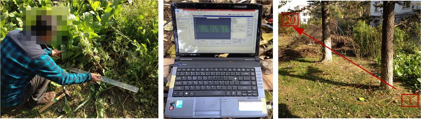
248                                       S. He et al.: A SSIP noise reduction algorithm based on correlation identification

   The field of FDIP denoising has achieved quite good re-
sults through the constant research of experts and scholars.
There have been many algorithms that can be used to sup-
press the FDIP random noise (Mo et al., 2017), such as
smooth filter (Guo, 2017), Mean stack (Liu, 2015), digital fil-
ter (Meng et al., 2015), and robust stacking (Liu et al., 2016).
The smooth can effectively attenuate Gaussian noise, but the
impulsive interference with intense energy leaves the effec-
tiveness of this algorithm limited. Therefore, an effective at-
tenuating algorithm for background noise is still a challeng-
ing task for traditional noise suppression algorithms (Neela-
mani et al., 2008; Liu et al., 2017a). SSIP method also faces
the same issue (Liu and Chen, 2016; Liu et al., 2017b).            Figure 1. (a) The observation model of the four-electrode measure-
   Recently, the new algorithm based on a circular cross-          ment. (b) Its equivalent diagram.
correlation method, time-domain spectral induced polariza-
tion based on pseudorandom sequence (TSIP) algorithm, has
also been used to suppress the SSIP noise (Li et al. 2013;           Given this observation mode using low-power signals, the
Zhang et al., 2020). Due to its effective denoising ability, the   magnetotelluric system is a time-invariant system and let
identification method has gained more attention and devel-         us suppose thatHS (ω) is 1. Equation (1) can further be ex-
opment. However, the TSIP algorithm is restricted because          pressed as
the excitation signal is sensitive to the random noise. For this              Pui (ω) fft [Rui (τ )] U (ω)
problem, we propose an enhanced correlation identification         He (ω) =           =                =       ,                 (2)
                                                                              Pii (ω)   fft [Rii (τ )]   I (ω)
(ECI) algorithm for reducing the noise in SSIP data. The ECI
algorithm obtains cross-correlations between the transmitter       where fft[.] denotes fast Fourier transform (FFT), Rui (τ )
output signal, the excitation signal, and the response signal.     is the cross-correlation function of u(t) and i(t), Rii (τ )
The performance of the ECI algorithm is demonstrated on            is the autocorrelation function of i(t), U (ω) and I (ω) de-
both synthetic and field SSIP data. Experimental results show      pict the geometric factor defined by the frequency spectrum
that the ECI algorithm can effectively control the root mean       of u(t)and the frequency spectrum of i(t) respectively, and
square of noise (NRMS) increase, enhance its denoising per-        τ denotes time delay.
formance in background noise and improve the valid signal             In the practical field environment, this observation mode
preservation to display the actual location and shape of high-     is contaminated by the background noise, as shown in Fig. 2.
resistivity anomalies with higher resolution.                      The output of the sensors Ak (k = 1, 2, 3) can be expressed
                                                                   as
2     Theory
                                                                   y1 = uT (t) + n1 (t),                                         (3)
2.1    The TSIP theoretical model                                  y2 = u(t) + n2 (t),                                           (4)
                                                                   y3 = i(t) + n3 (t),                                           (5)
Figure 1 shows a traditional diagram of the electrical resis-
tivity survey. The transmitter output signal uT (t) is poured      where nk (t) is the background noise.
from electrode A to electrode B, the excitation signal i(t)           Therefore, according to Eq. (2), the formula of the TSIP
flows from electrode A to electrode B, and the response sig-       algorithm is given as
nal u(t) between the electrodes M and N is measured. To
simultaneously obtain the spectral response of subsurface at                 Py2 y3 (ω) fft Ry2 y3 (τ )
                                                                   He (ω) =               =
various frequencies, pseudorandom sequence based the exci-

                                                                             Py3 y3 (ω) fft Ry3 y3 (τ )
tation signal i(t) is considered. Thus, the spectral response of
                                                                             fft Rui (τ ) + Run2 (τ ) + Rin1 (τ )
subsurface be retrieved by the TSIP algorithm, and its spec-              =
tral response be expressed as (Li et al., 2013):                             fft Rii (τ ) + Rin1 (τ ) + Rn1 n1 (τ )
                                                                                     fft [Rui (τ )]
                Pui (ω)                                                   ≈                           .                   (6)
He (ω) =                    ,                               (1)              fft Rii (τ ) + Rn3 n3 (τ )
           Pii (ω) · PS (ω)
                                                                   Equation (6) demonstrates that the TSIP algorithm has a
where Pui (ω) is the cross-power spectral density of u(t)
                                                                   weak denoising effect when n3 (t) is the massive intense
and i(t), Pii (ω) the auto-power spectral density of i(t), and
                                                                   noise. In other words, the TSIP algorithm depends on the
PS (ω) is the impulse spectral response of the observing sys-
                                                                   energy intensity of n3 (t) present in i(t).
tem.

Nonlin. Processes Geophys., 28, 247–256, 2021                                            https://doi.org/10.5194/npg-28-247-2021
S. He et al.: A SSIP noise reduction algorithm based on correlation identification                                                249

Figure 2. Schematic diagram using the TSIP algorithm.

Figure 3. The schematic diagram of the ECI denoising model.

2.2   The ECI theoretical model

That the denoising ability of the TSIP algorithm is limited is
caused by that i(t) is sensitive to n3 (t). To solve this prob-
lem, the ECI algorithm is proposed in Fig. 3 and its derivation
process is as follows.
   Firstly, let us suppose that the telluric system is a time-
invariant system under low-power signals. For three sensor
output signals, their cross-correlation functions are the peri-
odic correlation functions of time τ . When the length of the         Figure 4. Schematic diagram of the instrument.
correlation window NT is specified, 0.0125 s in this exper-
iment. The cross-correlation functions can be expressed as
follows:                                                              Then the cross-power spectrum of Eqs. (9) and (10) can be
                                                                      written as following

Ry1 y2 (τ ) = E y1 (t)y2 (t − τ ) = RuT u (τ ) N + Rn1 n2 (τ ), (7)
                                                                   Py1 y2 (ω) ≈ PuT u (ω),                                    (11)
Ry1 y3 (τ ) = E y1 (t)y3 (t − τ ) = RuT i (τ ) N + Rn1 n3 (τ ), (8)
                                                                      Py1 y3 (ω) ≈ PuT i (ω).                                    (12)
where Rn1 n2 (τ ) and Rn1 n3 (τ ) are the cross-correlations of,      Finally, according to Eqs. (2) and (11), Eq. (12) can be ex-
n2 (t) and n3 (t) respectively, and τ is time delay that lies in      pressed as following
the range of −NT to NT.
   Figure 4 shows the schematic diagram of the ZW-CMDSII                         U (ω) U (ω)UT∗ (ω) PuT u (ω)
instrument (Zhang et al., 2014; He et al., 2014). As is known         He (ω) =         =              =
                                                                                 I (ω)   I (ω)UT∗ (ω)   PuT i (ω)
from the figure, we can conclude that uT (t) is mainly dis-
                                                                                 Py1 y2 (ω)   Py1 y2 (ω) −j (ϕy1y2 (ω)−ϕy1y3 (ω))
turbed by the floor noise energy of the instrument, and i(t)                 ≈              =            e                        (13)
and u(t) are mainly contaminated by environmental noise.                         Py1 y3 (ω)   Py1 y3 (ω)
The floor noise is relatively very low, while environmental
                                                                      where ϕy1y2 (ω) and ϕy1y3 (ω) denotes the difference between
noise possesses a much higher energy level. Thus we assume
                                                                      y1 (t), y2 (t) and y3 (t).
that n1 (t) ≈ 0, and can conclude that zero correlation be-
                                                                         So, Eq. (13) is the formula of the ECI algorithm. The
tween n1 (t) and n2 (t), n3 (t), Rn1 n2 (τ ) ≈ 0 and Rn1 n3 (τ ) ≈
                                                                      derivation process of this formula clearly describes that the
0.
                                                                      ECI algorithm can effectively suppress the background noise
   Based on the above analyses, we can further obtain:
                                                                      and be independent on the degree of n3 (t) present in i(t).

Ry1 y2 (τ ) ≈ RuT u (τ ) N ,                                   (9)

Ry1 y3 (τ ) ≈ RuT i (τ ) N .                                  (10)

https://doi.org/10.5194/npg-28-247-2021                                           Nonlin. Processes Geophys., 28, 247–256, 2021
250 S. He et al.: A SSIP noise reduction algorithm based on correlation identification
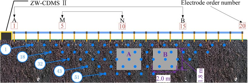
Figure 5. (a) Experimental schematic; (b) experimental setup.
3 Experiment on synthetic SSIP data record
We test the ECI algorithm for attenuating background noise
of SSIP data sets in comparison with the FDIP algorithm and
the TSIP algorithm. For the comparison, the signal-to-noise
ratio (SNR), root mean square of noise (NRMS), and rela-
tive error (ε) are the objective parameters to judge the perfor-
mance of denoising, which are calculated as follows:
M
P 2
y(i) − µy
i=1
SNR = 10log10 , (14)
M
[n(i) − µn ]2
P
i=1
v
uM
u [n(i)]2
uP
t i=1
NRMS = , (15)
M
ρ1 − ρ0
ε = 100 × , (16)
ρ0
i(t) = ui (t)/RS , (17)
where µy and µn denote the mean values of the useful signal
and the noise separately. y(i) and n(i) are the useful signal
and the noise separately, M is the length, ρ0 denotes the com-
plex resistivity calculated without noise, and ρ1 is the com-
plex resistivity calculated with the noise added to ρ0 . RS is
the value of the sampling resistor (RS = 1), and ui (t) is the
Figure 6. The time waves of (a) the applied voltage uT (t), (b) the
voltage at the sampling resistor.
measured potential signal u(t), (c) the voltage ui (t) at the sampling
To validate the effectiveness of the ECI system, we resistor, (d) noise (t), and (e) the synthetic signal (ui (t) + noise(t)).
performed a resistance–capacitance experiment, as shown
in Fig. 5. The circuit parameters are chosen to be
RA = 30.3 /5 W, RMN = 30.1 /5 W, RB = 30 /5 W, and
CMN = 470 µF. We recorded the applied voltage uT (t), the
Table 1. Amplitude and phase values of complex resistivity ob-
injected current i(t), and the measured potential signal u(t)
tained with Fig. 6a–c.
as the raw signals. These signals are a three-order spread
spectrum pseudorandom sequence at the clock cycle of
Frequency Theoretical Theoretical Measured Measured
0.0125 s, as shown in Fig. 6a–c and Table 1. (Hz) amplitude phase amplitude phase
Since our experiment is in a stable environment, we con- () (rad) () (rad)
sider the system to be linear time-invariant, and the noise
80.2 30.8 −0.14 30.8 −0.14
from the current and voltage measurements are linearly su-
160.4 30.4 −0.07 30.3 −0.08
perpositioned (Pelton and Sill, 1983; Vinegar and Waxman, 320.8 30.2 −0.03 30.7 −0.03
1984; Garrouch and Sharma, 1998). Therefore, it is actually
equivalent whenever the noise is added to the injected current
Nonlin. Processes Geophys., 28, 247–256, 2021 https://doi.org/10.5194/npg-28-247-2021
S. He et al.: A SSIP noise reduction algorithm based on correlation identification 251
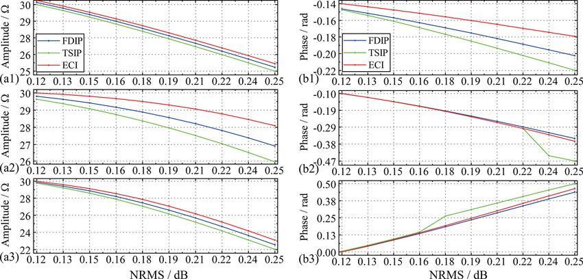
Figure 7. Amplitude and phase of complex resistivity values at (a1, b1) 80 Hz, and (a2, b2) 160 Hz, (a3, b3) 320 Hz using the three methods.
i(t), the measured potential signal u(t), or the applied volt-
age uT (t). Therefore, the injected current i(t) is only pol-
luted by the synthetic background noise, including Gaussian
and impulsive, as shown in Fig. 6d and e. Thirdly, the com-
plex resistivity of the main frequency is considered and dis-
cussed because the main energy of the pseudorandom signal
is concentrated on the main frequency (He, 2017). Finally,
Figure 8. The standard deviations (SDs) and skewness values (SKs)
for detailed comparisons between the ECI algorithm and the of synthetic impulsive noise.
others, we add the synthetic Gaussian and impulsive noises
to the response signal i(t), respectively.
We use synthetic Gaussian noise with the deviation and does not stand out, the overall change of the amplitude spec-
mean values of 0.1 and 1.1 as a standard template. The exci- trum after ECI processing is still slow, especially when the
tation signal i(t) is polluted by synthetic different energy lev- discrete point is more than 60 %.
els of the Gaussian noise. Figure 7 shows that the denoised
results are obtained and compared at the three main frequen-
cies when the NRMS ranges from 0.12 to 0.25. The figure
4 Experiment on real SSIP data record
shows that as the NRMS increases, the complex resistivity
information obtained by each algorithm decreases. However,
To further verify the performance of the ECI algorithm, the
the amplitude spectrum after ECI processing has the slowest-
Wenner array, which is the traditionally applied system in
falling speed, and the phase spectrum has the slowest-falling
the field, was selected for performing laboratory tests, as
speed at 80 Hz.
shown in Figs. 10 and 11. SSIP data was acquired with a
Previous literature has shown that if the percentages of
high-density meter and 20 electrodes at 1 m spacing. A Wen-
outliers in impulsive noise exceed 50 %, the traditional de-
ner acquisition sequence was adopted with 55 potential mea-
noising algorithm will be limited (Liu and Chen, 2016; Liu
surements expressed using the green points. The figure shows
et al., 2017a). Thus, synthetic impulsive noise is added to
an example of two high-resistance cavities. The two cavities
the excitation signal i(t) in 10 % steps. Their standard devi-
were presented by the letters A and B, and their calibers were
ations (SDs) and skewness values (SKs) are shown in Fig. 8.
about 1.8 m × 2 m. The two cavities are buried by loess. The
As depicted in Fig. 9, the three algorithms have a certain de-
loess is measured to have an electronic resistivity of 36 m.
gree of denoising performance versus the different percent-
The measured excitation signal had a range between 0.04
ages of the synthetic outliers against the raw data. The figure
and 0.19 A approximately. The transmitter output signal is
shows that with the discrete points of impulse noise growing,
a three-order sequence with 80 Hz frequency, and its voltage
the NRMS is different. The amplitude spectrum and phase
is about ±11.8 V. The sampling frequency is 625 kHz. The
spectrum of complex resistivity obtained by each algorithm
excitation and response data of 40 periods were recorded at
fluctuate. The amplitude spectrum after ECI processing re-
each point.
mained the slowest-falling speed. Although the noise reduc-
Figure 12 demonstrates the experimental SSIP data pro-
tion performance of the phase spectrum processed by ECI
cessed by the three algorithms, inverted with Res2DInv (Ar-
https://doi.org/10.5194/npg-28-247-2021 Nonlin. Processes Geophys., 28, 247–256, 2021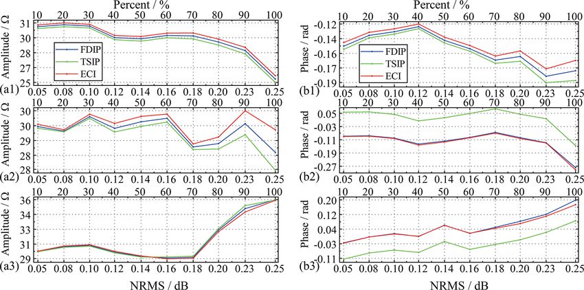
252                                         S. He et al.: A SSIP noise reduction algorithm based on correlation identification

Figure 9. Complex resistivity values at (a1, b1) 80 Hz, (a2, b2) 160 Hz, and (a3, b3) 320 Hz using the three methods.

Figure 10. Diagram of the field test.

Figure 11. The schematic of the two high-resistance cavities.

ifin et al., 2019). It can be observed that the location and            and 1.4 % lower than the others, and the minimum value is
shape of two abnormal bodies are distinguished only in the              8 % and 10 % lower, respectively.
ECI algorithm while recognized as one whole in the other                   Meanwhile, amplitude–frequency |ρ(f )| and phase–
algorithms. We believe the reason that ECI has higher detec-            frequency ϕ(f ) characteristics of complex resistivity are cal-
tion precision is due to its higher denoising ability.                  culated by the three algorithms (one period) in survey point
   To verify the reason for the improved detecting precision,           no. 38 in Fig. 11.
the SDs of data points are calculated from 18 to 50 (Fig. 11),             For example, Fig. 14a1 and a2 show that the amplitude
as shown in Fig. 13. This figure shows that the 33 SD in ECI            and phase of the complex resistivity spectrum for this point
processing the SSIP data is the lowest at all points. The aver-         at 80 Hz processed by FDIP are 39.7 m and −0.0881 rad,
age SD values in ECI processing of the SSIP data are 7 % and            the amplitude and phase are 40.9 m and 6.12 rad when
3.8 % lower than the FDIP and TSIP methods, respectively.               at 160 Hz, and the amplitude and phase are 38.7 m and
Also, the maximum value of SDs with the ECI method is 5 %               −0.253 rad when at 320 Hz. As depicted in Fig. 14, the

Nonlin. Processes Geophys., 28, 247–256, 2021                                               https://doi.org/10.5194/npg-28-247-2021
S. He et al.: A SSIP noise reduction algorithm based on correlation identification                                                  253

Figure 12. Inverted resistivity sections of the two high-resistivity anomalies (A and B) at 80 Hz with using (a) the FDIP method, (b) the
TSIP algorithm, and (c) the ECI algorithm.

Figure 13. Standard deviation (SD) values of the ECI algorithm and the others compared to the data dots from 18 to 50 at 80 Hz.

complex resistivity processed by the ECI shows a linear                noise reduction when the discrete point is more than 60 %,
trend with the three main frequencies. Also, the SD of the             which compensates for the disadvantage of the traditional
amplitude–frequency |ρ(f )| characteristic is 0.10 and 0.49            denoising algorithm. Moreover, these simulation results also
lower than the others, and the SD of the phase–frequency               reveal that the ECI algorithm should have high robustness.
ϕ(f ) is 3.56 and 0.03 lower. Therefore, we believe that the              The standard deviation analysis of the real data indicates
ECI algorithm has an advantage in suppressing background               that the ECI algorithm improves the accuracy and robustness
noise, which benefits the subsequent steps in SSIP data pro-           of the collected data, which are compatible with the simula-
cessing and imaging.                                                   tion analyses. This consistency shows that the ECI algorithm
                                                                       can obtain the location and shape of two abnormal bodies
                                                                       by improving the SNR of SSIP data, which can increase the
5   Discussion                                                         resolution of inversion results.

The simulation results indicate that the ECI algorithm has
very good performance in noise reduction and robustness.               6   Conclusions
Along with the increase of the Gaussian noise level, we found
that the ECI algorithm can, to some extend, overcome the               We propose the ECI algorithm that effectively attenuates the
shortcomings of the TSIP algorithm has, i.e., being suscep-            background noise in SSIP data and improves the complex re-
tible to the noise of the current. This result coincided with          sistivity spectrum. This algorithm uses the correlation func-
Eqs. (6) and (13), which provides a novel approach for cor-            tion to neutralize the influence of the background noise in the
related identification noise reduction. In the impulsive noise         SSIP data, and the spectrum complex resistivity can be calcu-
experiment, we found that the ECI algorithm still has good             lated at multiple frequencies by the formula of the complex

https://doi.org/10.5194/npg-28-247-2021                                             Nonlin. Processes Geophys., 28, 247–256, 2021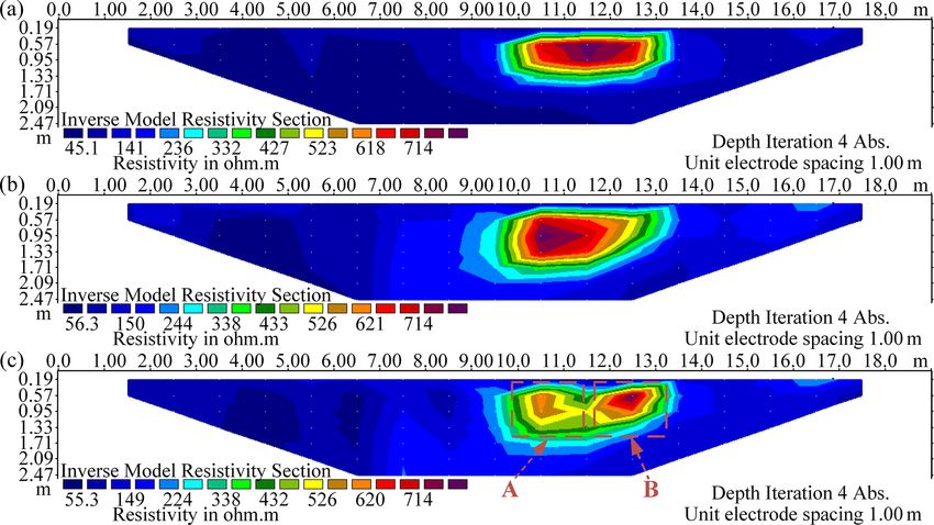
254                                            S. He et al.: A SSIP noise reduction algorithm based on correlation identification

Figure 14. Complex resistivity spectrum calculated by the three algorithms (one period) in survey point no. 38.

resistivity. Simulation results show that the ECI algorithm               Acknowledgements. We are grateful for the help of Jun Wang, Shi
can effectively attenuate the background noise and improve                Zhu, Hui Wang, and Jinshi Cui. We thank the editors and the re-
the SNR. Subsequently, the practicability of the ECI algo-                viewers for the constructive comments that helped to improve this
rithm is further verified by a field test. The results demon-             article.
strate that the SD of the SSIP data is improved, which ben-
efits the accuracy and stability of the collected data. There
is a good agreement between the complex resistivity and the               Financial support. This research has been supported by the Key
                                                                          Technology Projects of Science and Technology Department
geological target body with high resistance, which indicates
                                                                          of Jilin Province Scientific (grant no. 20190303015SF), a re-
that the ECI algorithm can help to improve the quality of in-
                                                                          search project of Jilin Provincial Department of Education (grant
terpretation and inversion in the survey area. For the ampli-             nos. JJKH20210692KJ and JJKH20211053KJ), and the Fundamen-
tude spectrum, the ECI algorithm can more effectively sup-                tal Research and Theme Funds for Changchun Institute of Technol-
press the background noise, including the Gaussian random                 ogy, China.
and impulsive noises. Still, its effect is very limited for the
phase spectrum. Therefore, a denoising algorithm based on
pseudorandom sequence correlation identification is still left            Review statement. This paper was edited by Richard Gloaguen and
open for more investigation.                                              reviewed by three anonymous referees.

Code availability. The code is a collection of routines in MATLAB
(MathWorks) and is available upon request to the author (e-mail:          References
hsmfly1982@163.com).
                                                                          Arifin, M. H., Kayode, J. S., Izwan, M. K., Zaid, H. A. H., and
                                                                            Hussin, H.: Data for the potential gold mineralization mapping
Data availability. All the SSIP data are collected by the ZW-               with the applications of Electrical Resistivity Imaging and In-
CMDSII and are available upon request to the author (e-mail: hsm-           duced Polarization geophysical surveys, Data in Brief, 22, 830–
fly1982@163.com).                                                           835, https://doi.org/10.1016/j.dib.2018.12.086, 2019.
                                                                          Chen, R. J., Luo, W. B., and He, J. S.: High precision
                                                                            multi-frequency multi-function receiver for electrical explo-
Author contributions. SH and YW designed the study, performed               ration, 2007 8th International Conference on Electronic
the research, analyzed data, and wrote the paper. JG contributed to         Measurement and Instruments (ICEMI’07), 16–18 August
language polishing and response. XJ and HX contributed to refining          2007, Xian, China, IEEE, Expanded Abstracts, 599–602,
the ideas, carrying out additional analyses, and finalizing this paper.     https://doi.org/10.1109/icemi.2007.4350521, 2007.
                                                                          Collett, L. S., Brant, A. A., Bell, W. E., Ruddock, K. A., Seigel,
                                                                            H. O., and Wait, J. R.: Laboratory investigation of overvolt-
                                                                            age, Overvoltage research and geophysical applications, Interna-
Competing interests. The authors declare that they have no conflict
                                                                            tional series of monographs on earth sciences, Pergamon, New
of interest.
                                                                            York, USA, 50–70, https://doi.org/10.1016/b978-0-08-009272-
                                                                            0.50009-1, 1959.

Nonlin. Processes Geophys., 28, 247–256, 2021                                                https://doi.org/10.5194/npg-28-247-2021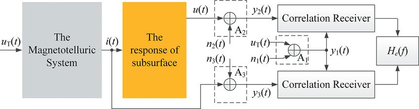
S. He et al.: A SSIP noise reduction algorithm based on correlation identification                                                         255

Garrouch, A. A. and Sharma M. M.: Dielectric dispersion of par-           Geophysics, 82, E243–E256, https://doi.org/10.1190/geo2016-
   tially saturated porous media in the frequency range 10 Hz to          0109.1, 2017a.
   10 MHz, The Log Analyst, 39, 48–53, 1998.                            Liu, W. Q., Wang, J. L., and Lin, P. R.: Signal processing approaches
Guo, H.: Study of key technology and data fusion of multi-probe           to obtain complex resistivity and phase at multiple frequencies
   penetration based on gas hydrate exploration, PhD Thesis, China        for the electrical exploration method, B. Geofis. Teor. Appl., 58,
   University of Geosciences, Wuhan, China, 2017.                         103–114, https://doi.org/10.4430/bgta0190, 2017b.
Han, S. L., Zhang, S. G., Liu, J. X., Hu, J., and Zhang, W.             Liu, W. Q., Lü, Q. T., Chen, R. J., Lin, P. R., Chen, C. J., Yang,
   S.: Integrated interpretation of dual frequency induced po-            L. Y., and Cai, H. Z.: A modified empirical mode decomposition
   larization measurement based on wavelet analysis and metal             method for multiperiod time-series detrending and the applica-
   factor methods, T. Nonferr. Metal. Soc., 23, 1465–1471,                tion in full-waveform induced polarization data, Geophys. J. Int.,
   https://doi.org/10.1016/S1003-6326(13)62618-7, 2013.                   217, 1058–1079, https://doi.org/10.1093/gji/ggz067, 2019.
He, G.: Wide area electromagnetic method and pseudo random sig-         Lu, Q. T., Zhang, X. P., Tang, J. T., Jin, S., Liang, L. Z., Wang, X.
   nal method, Higher Education Press, Beijing, China„ 2017.              B., Lin, P. R., Yao, C. L., Gao, W. l., Gu, J. S., Han, L. G., Cai, Y.
He, G., Wang, J., Zhang, B. Y., Li, M., and Ma, C.:                       Z., Zhang, J. C., Liu, B. L., and Zhao, J. H.: Review on advance-
   Design of High-density Electrical Method Data Acquisi-                 ment in technology and equipment of geophysical exploration for
   tion System, Instrument Technique and Sensor, 8, 18–19,                metallic deposits in china, Chinese J. Geophys., 62, 3629–3664,
   https://doi.org/10.3969/j.issn.1002-1841.2014.08.007, 2014.            https://doi.org/10.6038/cjg2019N0056, 2019 (in Chinese).
He, J. H., Yang, Y., Li, D. Q., and Weng, J. B.: Wide field elec-       Meng, Q. X., Pan, H. P., and Luo, M.: A study on the dis-
   tromagnetic sounding methods, in: Symposium on the Applica-            crete image method for calculation of transient electromag-
   tion of Geophysics to Engineering and Environmental Problems           netic fields in geological media, Appl. Geophys., 12, 493–502,
   (SAGEEP 2015), 22–26 March 2015, Texas, USA, EEGS, Ex-                 https://doi.org/10.1007/s11770-015-0517-x, 2015.
   panded Abstracts, 325–329, https://doi.org/10.4133/sageep.28-        Mo, D., Jiang, Q. Y., Li, D. Q., Chen, C. J., Zhang, B. M., and Liu, J.
   047, 2015.                                                             W.: Controlled-source electromagnetic data processing based on
He, J. S.: Dual-frequency IP, T. Nonferr. Metal. Soc., 3, 1–10, 1993.     gray system theory and robust estimation, Appl. Geophys., 14,
Høyer, A. S., Klint, K. E. S., Fiandaca, G., Maurya, P. K., Chris-        570–580, https://doi.org/10.1007/s11770-017-0646-5, 2017.
   tiansen, A. V., Balbarini, N., Bjerg, P. L., Hansen, T. B., and      Neelamani, R., Baumstein, A. I., Gillard, D. G., Hadidi, M. T.,
   Møller, I.: Development of a high-resolution 3D geological             and Soroka, W. L.: Coherent and random noise attenuation us-
   model for landfill leachate risk assessment, Eng. Geol., 249, 45–      ing the curvelet transform, The Leading Edge, 27, 240–248,
   59, https://doi.org/10.1016/j.enggeo.2018.12.015, 2018.                https://doi.org/10.1190/1.2840373, 2008.
Kimiaefar, R., Siahkoohi, S. H., Hajian, A., and Kalhor, A.: Random     Pelton, W. H. and Sill, W. R.: Interpretation of complex resistiv-
   noise attenuation by Wiener-ANFIS filtering, J. Appl. Geophys.,        ity and dielectric data, Geophysical Transactions, 29, 297–330,
   159, 453–459, https://doi.org/10.1016/j.jappgeo.2018.05.017,           1983.
   2018.                                                                Revil, A., Karaoulis, M., Johnson, T., and Kemna, A.: Review:
Li, G., Liu, X., Tang, J., Li, J., Ren, Z., and Chen, C.: De-noising      Some low-frequency electrical methods for subsurface character-
   low-frequency magnetotelluric data using mathematical mor-             ization and monitoring in hydrogeology, Hydrogeol. J., 20, 617–
   phology filtering and sparse representation, J. Appl. Geophys.,        658, https://doi.org/10.1007/s10040-011-0819-x 2012.
   172, 103919, https://doi.org/10.1016/j.jappgeo.2019.103919,          Revil, A., Razdan, M., Julien, S., Coperey, A., Abdulsamad,
   2019.                                                                  F., Ghorbani, A., and Rossi, M.: Induced polarization re-
Li, M., Wei, W., Luo, W., and Xu, Q: Time-domain spectral induced         sponse of porous media with metallic particles – Part
   polarization based on pseudo-random sequence, Pure Appl.               9: Influence of permafrost, Geophysics, 84, E337–E355,
   Geophys., 170, 2257–2262, https://doi.org/10.1007/s00024-012-          https://doi.org/10.1190/geo2019-0013.1, 2019.
   0624-z, 2013.                                                        Seigel, H. O.: Mathematical formulation and type curves
Liu, N.: Preprocessing and Research of denosing methods for ma-           for induced polarization, Geophysics, 24, 547–565,
   rine controlled source electromangnetic data, MSc Thesis, Jilin        https://doi.org/10.1190/1.1438625, 1959.
   University, Jilin, China, 2015.                                      Vinegar, H. J. and Waxman, M. H.: Induced polar-
Liu, W. Q. and Chen, R. J.: Coherence analysis for multi-frequency        ization of shaly sands, Geophysics, 49, 1267–1287,
   induced polarization signal processingin strong interference en-       https://https://doi.org/10.1190/1.1441755, 1984.
   vironment, The Chinese Journal of Nonferrous Metals, 26, 655–        Wang, Y. B. and He, J. S.: A hybrid coding and its ap-
   665,      https://doi.org/10.19476/j.ysxb.1004.0609.2016.03.022,       plication to the oil and gas fracturing intelligent real
   2016 (in Chinese).                                                     time monitoring system based on pseudorandom signal,
Liu, W. Q., Chen, R. J., Cai, H. Z., and Luo, W. B.: Robust sta-          Geophysical and Geochemical Exploration, 44, 74–80,
   tistical methods for impulse noise suppressing of spread spec-         https://doi.org/10.11720/wtyht.2020.2288, 2020.
   trum induced polarization data, with application to a mine           Wait, J. R.: The variable-frequency method, Overvoltage
   site, Gansu province, China, J. Appl. Geophys., 135, 397–407,          research and geophysical applications, International se-
   https://doi.org/10.1016/j.jappgeo.2016.04.020, 2016.                   ries of monographs on earth sciences, Pergamon, 29–49,
Liu, W. Q., Chen, R. J., Cai, H. Z., Luo, W. B., and Revil, André:        https://doi.org/10.1016/b978-0-08-009272-0.50008-x, 1959.
   Correlation analysis for spread spectrum induced polarization        Xi, X. L., Yang, H. C., He, L. F., and Chen, R. J.: Chromite mapping
   signal processing in electromagnetically noisy environments,           using induced polarization method based on spread spectrum
                                                                          technology, Symposium on the Application of Geophysics to

https://doi.org/10.5194/npg-28-247-2021                                              Nonlin. Processes Geophys., 28, 247–256, 2021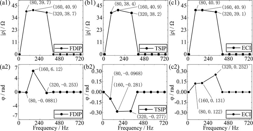
256                                        S. He et al.: A SSIP noise reduction algorithm based on correlation identification

  Engineering and Environmental Problems (SAGEEP 2013), 17–          Zhang, Q. D., Hao, K. X., and Li, M.: Improved correlation iden-
  21 March 2013, Denver, Colorado, USA, EEGS, Expanded Ab-             tification of subsurface using all phase FFT algorithm, KSII
  stracts, 13–19, https://doi.org/10.4133/sageep2013-015.1, 2013.      Transactions on Internet & Information Systems, 14, 495–513,
Xi, X. L., Yang, H. C., Zhao, X. F., Yao, H. C., Qiu, J. T.,           https://doi.org/10.3837/tiis.2020.02.002, 2020.
  Shen, R. J., and Chen, R. J.: Large-scale distributed 2D/3D        Zonge, K. L. and Wynn, J. C.: Recent advances and applications
  FDIP system based on ZigBee network and GPS, Symposium               in complex resistivity measurements, Geophysics, 40, 851–864,
  on the Application of Geophysics to Engineering and Environ-         https://doi.org/10.1190/1.1440572, 1975.
  mental Problems (SAGEEP 2014), 16–20 March 2014, Boston,
  Massachusetts, USA, EEGS, Expanded Abstracts, 130–139,
  https://doi.org/10.1190/SAGEEP.27-055, 2014.
Zhang, B. Y., He, G., and Wang J.: New High-density Electrical In-
  strument Measuring System, Instrument Technique and Sensor,
  1, 24–26, https://doi.org/10.3969/j.issn.1002-1841.2014.01.009,
  2014.

Nonlin. Processes Geophys., 28, 247–256, 2021                                           https://doi.org/10.5194/npg-28-247-2021
You can also read