An ARIMA analysis of the Indian Rupee/USD exchange rate in India
←
→
Page content transcription
If your browser does not render page correctly, please read the page content below
Munich Personal RePEc Archive

An ARIMA analysis of the Indian
Rupee/USD exchange rate in India

NYONI, THABANI

University of Zimbabwe, Department of Economics

3 November 2019

Online at https://mpra.ub.uni-muenchen.de/96908/
MPRA Paper No. 96908, posted 16 Nov 2019 11:01 UTC
AN ARIMA ANALYSIS OF THE INDIAN RUPEE/USD EXCHANGE RATE IN INDIA

                               1
Thabani NYONI1                  Faculty of Social Studies Department of Economics University of
                               Zimbabwe Harare, Zimbabwe, Email: nyonithabani35@gmail.com

                                         ABSTRACT
Keywords
ARIMA                          This study uses annual time series data on the Indian Rupee / USD exchange rate from
Exchange rate
Forecasting                    1960 to 2017, to model and forecast exchange rates using the Box-Jenkins ARIMA
India.                         technique. Diagnostic tests indicate that R is an I (1) variable. Based on Theil’s U, the
Indian Rupee/USD
                               study presents the ARIMA (0, 1, 6) model, the diagnostic tests further show that this
                               model is quite stable and hence acceptable for forecasting the Indian Rupee / USD
JEL Classification:            exchange rates. The selected optimal model the ARIMA (0, 1, 6) model shows that the
C53, E37, E47, F31, F37, O24
                               Indian Rupee / USD exchange rate will appreciate over the period 2018 – 2022, after
                               which it will depreciate slightly until 2027. The main policy prescription emanating from
                               this study is that the Reserve Bank of India (RBI) should devalue the Rupee, firstly to
                               restore the much needed exchange rate stability, secondly to encourage local
                               manufacturing and thirdly to promote foreign capital inflows.

Contribution/Originality:
This paper’s primary contribution is finding that the Indian Rupee/USD exchange rate will appreciate over
the period 2018 – 2022, after which it will depreciate slightly until 2027.
1. INTRODUCTION
     Exchange rate is an important variable which influences decisions taken by the participants of the foreign
exchange market, namely investors, importers, exporters, bankers, financial institutions, business, tourists and policy
makers both in the developing and developed world as well (Dua and Ranjan, 2011). Forecasting of the exchange rate
is essential for practitioners and researchers in the spree of international finance, particularly in the case of exchange
rate which is floating (Hu, 1999). Since the breakdown of the Bretton Woods System of fixed exchange rate in 1973,
the difficulty and desirability of obtaining reliable forecasts of exchange rates was highly demanding to earn income
from speculative activities, to determine optimal government policies as well as to make business decisions (Newaz,
2008). The foreign exchange market in India is believed to have begun in 1978 when the government allowed banks
to trade foreign exchange with each other. Today, it is almost unnecessary to reiterate the observation that
globalization and liberalization have significantly enhanced the scope for the foreign exchange market in India. The
Indian exchange rate is regime, as noted by Goyal (2018) is a managed float, where the central bank allows markets
to discover the equilibrium level but only intervenes to prevent excessive volatility.
1.1. Research Objectives
    i.    To develop an optimal ARIMA model for the analysis of the Indian Rupee / USD exchange rate.
    ii.   To check whether the Random Walk Model out performs other ARIMA processes in forecasting the Indian
          Rupee / USD exchange rate.
   iii.   To predict the Indian Rupee / USD exchange rate over the period 2018 – 2027
1.2. Statement of the Problem
     Foreign exchange markets are filled with uncertainty (Canova and Marrinan, 1993). Foreign exchange traders are
constantly looking for ways to protect themselves against these uncertainties and unwanted fluctuations due to the
effect that they have on the economic outlook of a country (Gali and Monacelli, 2005). There is no doubt; exchange
rate stability contributes to the development of a safe macroeconomic environment which leads to growth and
investment (Ames et al., 2001). A number of forecasting techniques have been developed and yet the much needed
exchange rate stability has not materialized (Tudela, 2004). It is important to understand how the exchange rate
mechanism works and contributions can be made to any forecasting model so as to reach the desired level of
confidence and trust the market needs (Grauwe and Schnabl, 2008). The importance of forecasting exchange rates in

                                                                                                                           1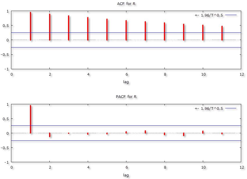
practical aspect is that an accurate forecast can render valuable information to the investors, firms and central banks
for use in allocation of assets, in hedging risk and in policy formulation (Tindaon, 2015). The modeling and
forecasting of the Indian Rupee / USD Exchange Rate is expected to go a long way in improving policy formulation
in India.
2. LITERATURE REVIEW
2.1. Theoretical Literature Review
      There are a number of theories of exchange rate determination, applied in exchange rate forecasting; in this study
we will only consider three of them:
2.2. The Purchasing Power Parity (PPP) Model
      The PPP framework, officially named and popularized by Cassel (1918) is an exchange rate model which is
based on the famous “law of one price” and explains the movements of the exchange rate between two countries’
currencies by the changes in the countries’ price levels. The basic argument is that the goods-market arbitrage
mechanism will move the exchange rate to equalize prices in the two countries. For example, if the United States
(US) goods are more expensive than those in India, consumers in the US and India may tend to purchase more Indian
goods. The increased demand for Indian goods will drive the Indian Rupee to appreciate with respect to the USD until
the dollar-denominated prices of the US goods and Indian goods are equalized. The PPP model can be expressed as
follows:

                                                                                                           (1)

 where      is the nominal exchange rate,      and      are domestic and foreign prices respectively. Equation (1) is

reffered to as the relative version of the PPP model, since price indices instead of actual price levels are used in
estimations. Equation (1) is a “weaker” variation of the PPP theory, hence the term relative PPP theory and is
different from the absolute version of the PPP theory which is based on a strict interpretation of the law of one price.
However, the absolute PPP theory is unlikely to hold, probably due to the existence of transport costs, imperfect
information as well as distorting effects of tariffs and other forms of protectionism and yet the relative PPP theory
arguably holds even in the presence of such distortions. It is almost unnecessary to note that equation (1) points to the
notion that the exchange rate will adjust by the amount of the inflation differential between two economies. However,
the applicability of the PPP theory in exchange rate determination is subject to a hot debate, for example, Enders
(1988); Corbae and Ouliaris (1990) and Tronzano (1992) amongst other argue that the PPP theory performs poorly
while, on the other side of the same coin, researchers such as Abuaf and Jorion (1990); Kim (1990); Patel (1990) and
Taylor (1990) have found out that the PPP theory is applicable, especially in developed countries and can therefore
forecast exchanges very well, especially for the long-run.
2.3. The Uncovered Interest Rate Parity (UIP) Model
      The UIP explains how the exchange rate moves according to the expected returns of holding assets in two
different currencies. UIP ignores transaction costs and liquidity constraints and apparently gives an arbitrage
mechanism that drives the exchange rate to a value that equalizes the returns on holding both the domestic and
foreign assets. If the UIP holds, the arbitrage relationship gives the following expression:

                                                                                                                 (2)

where                           is the market expectation of the exchange rate return from time t to time t+h, and

and      are interest rates of the domestic and foreign currencies respectively. Uncovered interest parity condition, as

                                                                                                                       2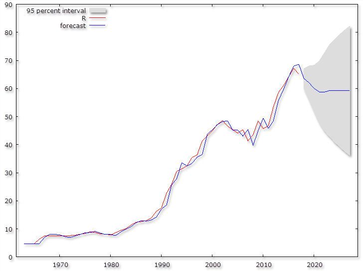
presented in equation (2), implies that market arbitrage will move the exchange rate to the point at which the expected
rate of return on investments denominated in either the home or foreign currency is the same, with the exception of a
possible risk premium. Essentially, equation (2) rules out the possibility of excess profits in asset markets, in the
sense that the interest rate differential between the home and foreign country equals the anticipated change in the
exchange rate. The applicability of the UIP model in forecasting exchange rates has been shown by Meredith and
Chinn (1998); Alexius (2001) and Cheung et al. (2004) who noted that the UIP model is basically capable for
forecasting at longer horizons.
2.4. The Sticky Price Monetary (SPM) Model
    The SPM model, postulated by Dornbusch (1976) and Frankel (1979) is basically an extension of the PPP model
by replacing the price variables in equation (Abdullah et al., 2017) with macroeconomic variables that capture money
demand and over-shooting effects. Frankel (1979) specifies the SPM model as follows:

                                                                                                                (3)

where      is the domestic money supply,        is the domestic output,     is the domestic interest rate,    is the domestic

current state of expected long run inflation, and all variables in asterisk denote variables of the foreign country.
Equation (3) incorporates the short-run interest rate in order to capture liquidity effects and also assumes that the
expected rate of depreciation of the exchange rate is positively related to the gap between the current exchange rate
and the long-run equilibrium rate and the anticipated long-run inflation differential between the domestic and foreign
countries. Equation (3) can also be explained as an overshooting model in the sense that the exchange rate tends to
overshoot its new equilibrium level following some exogenous shock to the system. For instance, a shock which
warrants depreciation of the exchange rate to a new long run level: overshooting means that in the short run, the
exchange rate has a tendency of over-depreciating before appreciating towards its new long run equilibrium value.
2.5. Empirical Literature Review
    A myriad of scholarly papers have been published on the area of exchange rate forecasting since the breakdown
of the Bretton Woods System. Given the main thrust of this paper, Table 1 below provides a fair sample of relevant
studies undertaken more recently:

                                              Table-1. Reviewed Previous Studies
 Author(s)/Year                    Country          Period                Methodology           Main Findings
 Alam (2012)                       Bangladesh       July 2006 – April     AR,    ARIMA,         AR and ARMA models
                                                    2010                  ARMA, MA              outperform other models
 Pacelli (2012)                    Italy            January 1999 –        ANN,    ARCH,         ARCH and GARCH
                                                    December 2009         GARCH                 models perform better
                                                                                                than ANN
 Ramzan et al. (2012)              Pakistan         1981 – 2010           ARIMA, ARCH,          GARCH (1, 2) is the best
                                                                          GARCH,                to remove the persistence
                                                                          EGARCH                in     volatility       while
                                                                                                EGARCH            (1,      2)
                                                                                                successfully       overcame
                                                                                                the leverage effect in the
                                                                                                exchange rate returns
 Pedram and Ebrahim (2014)         Iran             November 2010         ARIMA, ANN            ANNs are far much better
                                                    – June 2013                                 than ARIMA models
 Nwankwo (2014)                    Nigeria          1982 – 2011           ARIMA                 AR (1) model (i.e
                                                                                                ARIMA (1, 0, 0)) was the
                                                                                                best.
 Erdogan and Goksu (2014)          Turkey           2010 – 2013           ANN                   ANNs       can        closely
                                                                                                forecast     the       future
                                                                                                EUR/TRY exchange rates
 Babu and Reddy (2015)             India            January 2010 –        ARIMA, ANN,           ARIMA model performs
                                                    April 2015            Fuzzy Neuron          better than complex non-

                                                                                                                                3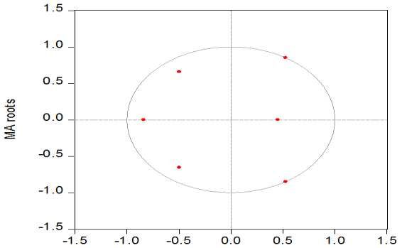
linear models
  Etuk and Natamba (2015)                     Nigeria       July 1990 –        SARIMA             SARIMA (0, 1, 1)(0, 1,
                                                            November 2014                         1)12, SARIMA (0, 1, 1)(1,
                                                                                                  1, 1)12 are preferred
  Gupta and Kashyap (2015)                    India         April 2014     –   ARIMA              The following models
                                                            March 2015                            were      found     to be
                                                                                                  performing very well:
                                                                                                  ARIMA (0, 1, 1),
                                                                                                  ARIMA (2, 1, 1) and
                                                                                                  ARIMA (2, 1, 2)
  Ngan (2016)                                 Vietnam       January 2013 –     ARIMA              VND/USD in 2016 tends
                                                            December 2015                         to increase
  Abdullah et al. (2017)                      Bangladesh    January 2008 –     GARCH,             AR (2) – GARCH (1, 1)
                                                            April 2015         APARCH,            is the best model
                                                                               TGARCH,
                                                                               IGARCH
  Qonita et al. (2017)                        Indonesia     January 2010 –     ARIMA              ARIMA method has an
                                                            June 2016                             accuracy rate of 98.74%
  Mustafa et al. (2017)                       Malaysia      November 2010      Hybrid ARIMA-      ARIMA-EGARCH
                                                            – August 2016      GARCH, hybrid      model fits the data better
                                                                               ARIMA-
                                                                               EGARCH
  Ganbold et al. (2017)                       Turkey        2005 – 2017        ARIMA,             EGARCH (1, 1) performs
                                                                               SARIMA,            better
                                                                               ARCH, SVAR
  Mia et al. (2017)                           Bangladesh    August 2004 –      ARIMA, ESM,        ANNs perform better
                                                            March 2016         ANN                than ARIMA models
  Nyoni (2018l)                               Nigeria       1960 – 2017        ARIMA              ARIMA (1, 1, 1) is the
                                                                                                  optimal model
Source: Authors’ analysis from literature review (2019).
3. METHODOLOGY
3.1. Autoregressive (AR) Models

A series           (which represents the Indian Rupee / USD exchange rate at time, t) is said to be an autoregressive

process of order p, denoted by AR (p) if it can be expressed in the form:

                                                                                                                (4)

Equation (4) implies that the Indian Rupee / USD exchange rate, in this regard, is explained by the previous period
values of the Indian Rupee / USD series, hence the term “autoregressive”.
Using the backshift operator, equation (4), as noted by (Alexius, 2001); can be written as:

                                                                                                                (5)

Where B is the backshift operator,                         are parameters of the model and   is a normally distributed random

process with mean 0 and a constant varience                   and is assumed to be independent of all previous process values

      AR models are normally restricted to stationary data (Hyndman and Athanasopoulos, 2014). Therefore, it is
necessary to check for stationarity of the data before fitting such models.

                                                                                                                               4
3.2. Moving Average (MA) Models
A series with a white noise process of mean 0 and varience is reffered to as a moving average process of
order q, denoted as MA (q), if it can be expressed as a weighted linear sum of past forecast errors as follows:
(6)
Equation (6) means that the Indian Rupee / USD exchange can be explained using the current and previous period
disturbances (the random errors, or the socalled shocks such as unanticipated political events).
In backshift operator notation, equation (6), as noted by (Alam, 2012); can be written as:
(7)
Where are coefficients of the lagged error terms and is assumed to be equal to 1. B and are as
previously defined.
The parameters of an MA process must be negative so that we can have characteristic operators of the same signs for
both AR and MA processes, although this has no significant change to the interpretation of the model.
3.3. Autoregressive Moving Average (ARMA) Models
Combining both the AR (p) and MA (q) models gives rise to an Autoregressive Moving Average model (ARMA
(p, q)) model which can be expressed as follows:
(8)
Equation (8) means that the Indian Rupee / USD exchange rate can be explained by its previous period values as well
as the current and past disturbances.
Re-arranging equation (8), as hinted by (Box and Jenkins, 1994); gives:
(9)
Using the backshift operator equation (Canova and Marrinan, 1993) can be expressed as follows:
(10)
Equation (10), based on (Cassel, 1918); can be simplified to:
(11)
Where:
(12)
5Both the AR (p) and MA (q) are special cases of the ARMA model. An ARMA (p, 0) process is the same as an
AR (p) process and an ARMA (0, q) process is the same as an MA (q) process. If the available data is stationary, it is
better modeled using an ARMA (p, q) model than AR (p) or MA (q) models individually (Chin and Fan, 2005). This
is because an ARMA (p, q) model in such as case uses fewer parameters than the individual models and gives a better
representation of the data and this is reffered to as the principle of parsimony (Singh, 2002; Woodward et al., 2011).
3.4. Autoregressive Integrated Moving Average (ARIMA) Models
Most time series data is not stationary due to seasonality and trend. Hence, once cannot apply AR, MA or ARMA
models directly. The best way of obtaining stationarity when dealing with ARIMA models is differencing
(Systematics, 1994). Basically, time series data can be differenced “d” times, until it becomes stationary. Most time
series data become stationary after differencing, either once or twice, and in that case, “d” is either 1 or 2,
respectively. By convention, differencing “d” times can be written as:
If the original data series is differenced “d” times before fitting an ARMA (p, q) model, then the model for the
original undifferenced series said to be an ARIMA (p, d, q), where “d” represents the number of times the data has
been differenced (Hendry, 1995).
Differencing “d” times changes equation (11), as suggested by (Cassel, 1918); to:
(13)
Equation (13), following (Chin and Fan, 2005); can be simplified to:
(14)
Equation (13), as noted by (Corbae and Ouliaris, 1990); is reffered to as an ARIMA model. The white noise
process (ARIMA (0, 0, 0)), random walk process (ARIMA (0, 1, 0)), autoregressive process (ARIMA (0, 0, q)) and
autoregressive moving average (ARIMA (p, 0, q)) are special types of ARIMA models.
3.5. The Random Walk Model – The ARIMA (0, 1, 0) Model
The random walk model can be given by:
(15)
where is as previously defined and apparently denotes a purely random process.
Equation (15) (Dornbusch, 1976) does not form a stationary process, however, the first difference: ,
forms a stationary series.
Equation (15) (Dornbusch, 1976) can also be decomposed as follows:
(16)
The mean function is given by:
6(17)
(18)
Equation (17) implies that, on average, all errors or disturbances or shocks, sum up to zero. Hence the process
varience increases with time, linearly as shown in equation (18).
Analysis of the Covariance Function
Given: , then:
(19)
This can be written as follows:
(20)
The covariates are normally equal to zero unless when i=j, and in that scenario, we have: . There are
t of these such that . The purpose of equations (15) to (20) is to uncover the issue of covariance
stationarity, which is an important issue when it comes to univariate analysis in econometrics. A stochastic process is
thought of as stationary if its mean and varience are constant over time and the value of the covariance between the
two time periods depends only on the gap or lag between the two periods and not the actual time at which the
covariance is computed. The simplest example of a covariance stationary stochastic process is a white-noise process.
Equation (17) is the mean function while equation (18) is varience function. Equations (19 – 20) show the covariance
functions and that the covariance function is stationary since the value of the covariance between period t and s
depends on the lag between the two periods and not the actual time at which the covariance is calculated.
3.6. The Box – Jenkins Technique
The first step towards model selection is to difference the series in order to achieve stationarity. Once this
process is over, the researcher will then examine the correlogram in order to decide on the appropriate orders of the
AR and MA components. It is important to highlight the fact that this procedure (of choosing the AR and MA
components) is biased towards the use of personal judgement because there are no clear – cut rules on how to decide
on the appropriate AR and MA components. Therefore, experience plays a pivotal role in this regard. The next step is
the estimation of the tentative model, after which diagnostic testing shall follow. Diagnostic checking is usually done
by generating the set of residuals and testing whether they satisfy the characteristics of a white noise process. If not,
there would be need for model re – specification and repetition of the same process; this time from the second stage.
7The process may go on and on until an appropriate model is identified (Nyoni, 2018i). The Box – Jenkins technique is
accredited to Box and Jenkins (1970) and is widely used in many forecasting contexts. In this paper, we will use it for
forecasting the Indian Rupee / USD exchange rates.
3.7. Data Collection
In line with Chatfield (1996) and Meyler et al. (1998) who argued that more than 50 observations are needed in
order to build a reliable ARIMA model, this study is based on a data set of the Indian Rupee / USD 1 exchange rate
(denoted as R) ranging over the period 1960 – 2017. All the data used in this study was extracted from the World
Bank online database.
3.8. Diagnostic Tests and Model Evaluation
3.1.8. Stationarity Tests: Graphical Analysis
Figure-1. Graphical Analysis
Source: Author’s Own Computation
3.9. The Correlogram in Levels
Figure-2. Correlogram in Levels
1
United States Dollar.
8Source: Author’s Own Computation
3.10. The ADF Test
Table-2. Levels-intercept.
Variable ADF Statistic Probability Critical Values Conclusion
Rt 1.594465 0.9994 -3.550396 @1% Not stationary
-2.913549 @5% Not stationary
-2.594521 @10% Not stationary
Source: Author’s Own Computation
Table-3. Levels-trend & intercept.
Variable ADF Statistic Probability Critical Values Conclusion
Rt -1.492394 0.8208 -4.127338 @1% Not stationary
-3.490662 @5% Not stationary
-3.173943 @10% Not stationary
Source: Author’s Own Computation
Table-4. without intercept and trend & intercept.
Variable ADF Statistic Probability Critical Values Conclusion
Rt 4.159 1.000 -2.606163 @1% Not stationary
-1.946654 @5% Not stationary
-1.613122 @10% Not stationary
Source: Author’s Own Computation
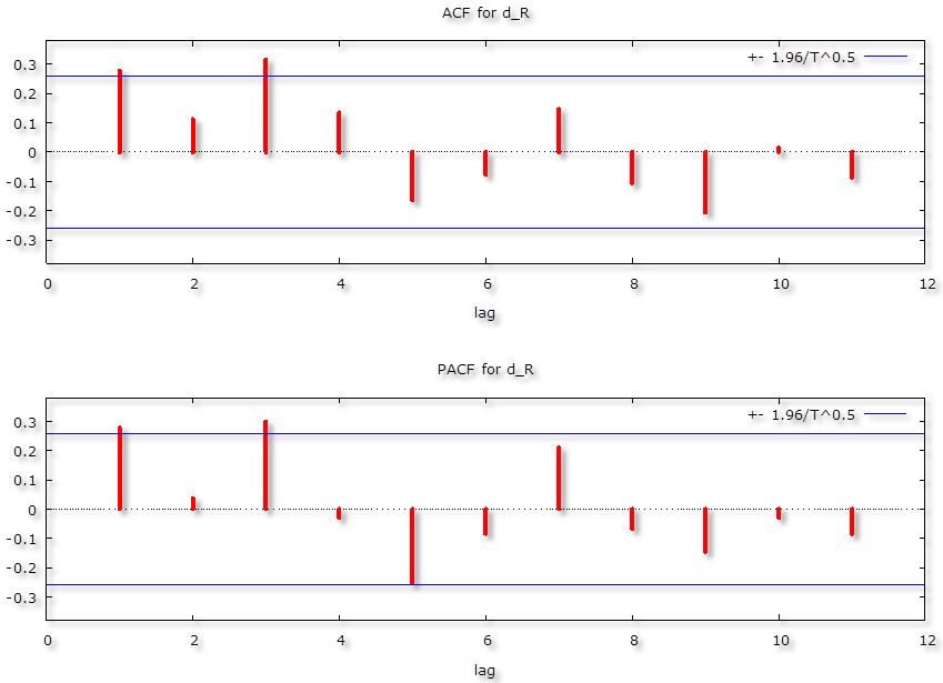
3.11. The Correlogram at 1st Differences
Figure-3. Correlogram in 1st Differences
Source: Author’s Own Computation
Table-5. 1st Difference-intercept.
Variable ADF Statistic Probability Critical Values Conclusion
D(Rt) -5.329250 0.0000 -3.552666 @1% Stationary
-2.914517 @5% Stationary
-2.595033 @10% Stationary
Source: Author’s Own Computation
Table-6. 1st Difference-trend & intercept.
Variable ADF Statistic Probability Critical Values Conclusion
D(Rt) -5.570223 0.0001 -4.130526 @1% Stationary
-3.492149 @5% Stationary
-3.174802 @10% Stationary
Source: Author’s Own Computation
9Table-7. 1st Difference-without intercept and trend & intercept.
Variable ADF Statistic Probability Critical Values Conclusion
D(Rt) -1.961682 0.0484 -2.608490 @1% Stationary
-1.946996 @5% Stationary
-1.612934 @10% Stationary
Source: Author’s Own Computation
Figures 1, 2 and 3 and Tables 2 to 7 indicate that R is an I (1) variable.
3.12. Evaluation of ARIMA Models (without a constant)
Table-8. Evaluation of ARIMA models
Model AIC U ME MAE RMSE MAPE
ARIMA (1, 1, 1) 243.6966 0.85192 0.37654 1.2341 1.9402 4.7461
ARIMA (0, 1, 2) 248.9982 0.88621 0.6934 1.349 2.0358 4.8727
ARIMA (0, 1, 1) 247.2181 0.89296 0.723 1.3598 2.0395 4.8946
ARIMA (0, 1, 3) 241.0277 0.87503 0.51926 1.2289 1.8535 4.899
ARIMA (0, 1, 4) 240.3721 0.85135 0.41417 1.1644 1.81 4.6827
ARIMA (0, 1, 5) 242.3710 0.85162 0.41753 1.1647 1.8101 4.6812
ARIMA (1, 1, 0) 245.3469 0.86294 0.56792 1.2857 2.0061 4.697
ARIMA (2, 1, 0) 246.4242 0.85609 0.50154 1.2545 1.9894 4.671
ARIMA (3, 1, 0) 240.4945 0.85664 0.35074 1.2009 1.8489 4.7601
ARIMA (4, 1, 0) 242.4934 0.85688 0.34981 1.2014 1.8489 4.7658
ARIMA (5, 1, 0) 241.6721 0.86423 0.38937 1.212 1.7994 4.8872
ARIMA (2, 1, 2) 246.0884 0.8434 0.36352 1.2081 1.9115 4.5822
ARIMA (0, 1, 6) 244.0862 0.84203 0.41489 1.1584 1.8012 4.6528
2
ARIMA (0, 1, 0) - 1 1.0589 1.5621 2.2498 5.7223
ARIMA (1, 1, 2) 245.4296 0.84583 0.34008 1.2492 1.9312 4.6125
ARIMA (1, 1, 3) 241.1691 0.85631 0.40144 1.1675 1.8231 4.7143
ARIMA (1, 1, 4) 242.3713 0.85154 0.41651 1.1646 1.8101 4.6817
ARIMA (2, 1, 1) 245.6751 0.85035 0.37414 1.2356 1.9399 4.7305
ARIMA (3, 1, 1) 242.4940 0.85675 0.35032 1.2012 1.8489 4.7627
ARIMA (4, 1, 1) 244.2591 0.85993 0.34178 1.2183 1.8448 4.846
ARIMA (5, 1, 1) 243.6160 0.86648 0.39433 1.2091 1.7984 4.8985
ARIMA (2, 1, 4) 244.3247 0.8518 0.44263 1.1663 1.8101 4.6637
Source: Author’s Own Computation
A model with a lower AIC value is better than the one with a higher AIC value (Nyoni, 2018n) Theil’s U must
lie between 0 and 1, of which the closer it is to 0, the better the forecast method (Nyoni, 2018l). In this paper, we rely
mainly on the Theil’s U as the criteria for choosing the best model. The Theil’s U indicates that the random walk
model performs poorly and is in fact, the worst, in the case of the Indian Rupee / USD exchange rate as shown in this
regard. This means that the annual Indian Rupee / USD exchange rate does not follow a random walk. This is
apparently inconsistent with Mussa (1979) and Meese and Rogoff (1983) who showed the superiority of the random
walk model in out-of-sample exchange rate forecast. However, the Theil’s U evaluation statistic shows that the
ARIMA (0, 1, 6) model outperforms other ARIMA models and is therefore chosen as the best model.
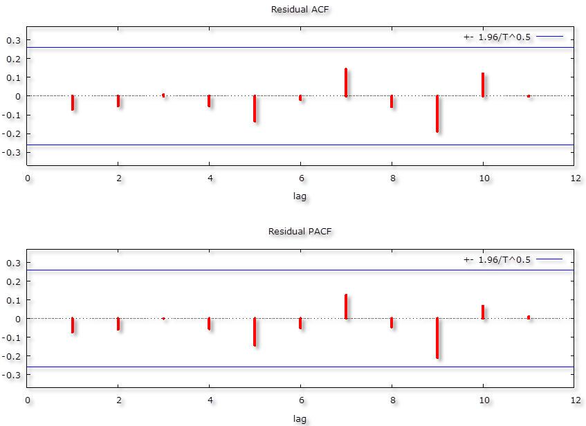
3.13. Residual & Stability Tests
3.13.1. Residual Correlogram of the ARIMA (0, 1, 6) Model
2
Random Walk Model
10Figure-4. Residual Correlogram
Source: Author’s Own Computation
3.14. ADF Tests of the Residuals of the ARIMA (0, 1, 6) Model
Table-9. Levels-intercept.
Variable ADF Statistic Probability Critical Values Conclusion
Rt -7.373411 0.0000 -3.552666 @1% Stationary
-2.914517 @5% Stationary
-2.595033 @10% Stationary
Source: Author’s Own Computation
Table-10. Levels-trend & intercept.
Variable ADF Statistic Probability Critical Values Conclusion
Rt -7.314221 0.0000 -4.130526 @1% Stationary
-3.492149 @5% Stationary
-3.174802 @10% Stationary
Source: Author’s Own Computation
Table-11. without intercept and trend & intercept.
Variable ADF Statistic Probability Critical Values Conclusion
Rt -7.077427 0.0000 -2.606911 @1% Stationary
-1.946764 @5% Stationary
-1.613062 @10% Stationary
Source: Author’s Own Computation
Figure 4 and Table 9 to Table 11 indicate that the residuals of the ARIMA (0, 1, 6) model are stationary.
3.15. Stability Test of the ARIMA (0, 1, 6) Model
Figure-5. Stability Test
Source: Author’s Own Computation
11Because the corresponding inverse roots of the characteristic polynomial lie in the unit circle, we can safely
conclude that the chosen ARIMA (0, 1, 6) model is indeed stable.
4. FINDINGS
Table-12. Descriptive Statistics
Description Statistic
Mean 25.647
Median 15.075
Minimum 4.76
Maximum 67.2
Standard deviation 19.986
Skewness 0.52602
Excess kurtosis -1.1889
Source: Author’s Own Computation
As shown in Table 12 above, the mean is positive, i.e 25.647. The median is 15.075. The maximum is 67.2. The
minimum is 4.76. Since skewness is 0.52602, it implies that variable R is positively skewed and non-symmetric.
Excess kurtosis is -1.1889 and simply indicates that R is not normally distributed.
4.1. Results Presentation3
Table-13. Results
ARIMA (0, 1, 6) Model:
(21)
Variable Coefficient Standard Error z p-value
0.375217 0.136507 2.749 0.0060***
0.232964 0.148769 1.566 0.1174
0.455302 0.152045 2.995 0.0027***
0.333495 0.156202 2.135 0.0328**
0.0486549 0.158404 0.3072 0.7587
-0.137725 0.148658 -0.9265 0.3542
Source: Author’s Own Computation
Equation (21) is the estimated optimal model, the ARIMA (0, 1, 6) model. Only are significant,
showing the importance of such disturbances or shocks (shocks experienced 1 year ago, 3 years ago as well as 4 years
ago) in explaining exchange rate movements in India over the study period.
3
***, ** and * means significant at 1%, 5% and 10% level of significance, respectively.
12Figure-6. Forecast Graph
Source: Author’s Own Computation
4
Table-14. Out-of-Sample Forecast
Year Predicted Indian Rupee / USD exchange rate Standard Error 95% interval
2018 63.5526 1.80003 (60.0246, 67.0806)
2019 62.0545 3.06071 (56.0556, 68.0534)
2020 60.0088 4.21280 (51.7518, 68.2657)
2021 58.8002 5.61640 (47.7922, 69.8081)
2022 58.7415 7.08238 (44.8603, 72.6227)
2023 59.2223 8.33905 (42.8781, 75.5665)
2024 59.2223 9.31655 (40.9622, 77.4824)
2025 59.2223 10.2008 (39.2291, 79.2155)
2026 59.2223 11.0143 (37.6347, 80.8099)
2027 59.2223 11.7717 (36.1502, 82.2944)
Source:
Figure-7. Graphical Presentation of the Out-of-Sample Forecast
Source: Author’s Own Computation
4
For 95% confidence intervals, z(0.025) = 1.96
13Table 13 shows the main results of the optimal model, the ARIMA (0, 1, 6) model. Only are
significant, indicating the importance of such shocks (shocks experienced 1 year ago, 3 years ago as well as 4 years
ago) in explaining exchange rate dynamics in India. Figures 6 & Figure 7 and Table 14 show the predicted Indian
Rupee / USD exchange rate over the period 2018 to 2027: the annual Indian Rupee / USD exchange rate is expected
to fall (appreciate) over the forecasted period. Our findings are partially consistent with Goyal (2018) who observed
that in 2017, the Indian Rupee / USD exchange rate appreciated. Our findings show that major appreciation will not
persist into the medium term but only occur over the period 2020 – 2022, after which the Indian Rupee / USD
exchange rate will start depreciating again. The Rupee, as argued by Goyal (2018) cannot appreciate substantially
unless the Renminbi does so, since China (and not the US) is a major trade competitor and partner.
5. CONCLUSION & POLICY IMPLICATIONS
Exchange rates have long fascinated, challenged and puzzled researchers in international finance (Zorzi et al.,
2015). Exchange rate prediction is one of the demanding applications of modern time series forecasting (Nwankwo,
2014). The rates are inherently noisy, non-stationary and deterministically chaotic (Box and Jenkins, 1994).
Generating quality forecasts is not an easy task (Mustafa et al, 2017). Given the analysis and forecasts of this study,
our recommendation is that policy makers in India ought to devalue the Rupee in order to restore and maintain
exchange rate stability. Once devaluation is implemented in India, the local manufacturing sector will grow
phenomenally and this is likely to be accompanied by inflows of the much awaited foreign capital.
REFERENCES
Abdullah, S., S. Siddiqua, M.S.H. Siddiquee and N. Hossain, 2017. Modeling and forecasting exchange rate volatility in
Bangladesh using GARCH models: A comparison based on normal and student’s t-error distribution. Financial
Innovation, 3(1): 1-19.Available at: https://doi.org/10.1186/s40854-017-0071-z.
Abuaf, N. and P. Jorion, 1990. Purchasing power parity in the long run. The Journal of Finance, 45(1): 157-174.
Alam, M.Z., 2012. Forecasting the BDT/USD exchange rate using autoregressive model. Global Journal of Management and
Business Research, 12(19): 84 – 96.
Alexius, A., 2001. Uncovered interest parity revisited. Review of International Economics, 9(3): 505-517.
Ames, B., W. Brown, S. Devarajan and A. Izquierdon, 2001. Macroeconomic policy and poverty reduction. Washington DC:
World Bank.
Babu, A.S. and S.K. Reddy, 2015. Exchange rate forecasting using ARIMA, neural network and fuzzy Neuron. Journal of Stock &
Forex Trading, 4(3): 1 – 5.Available at: http://dx.doi.org/10.4172/2168-9458.1000155.
Box, D.E. and G.M. Jenkins, 1970. Time series analysis, forecasting and control. London: Holden Day.
Box, G.E.P. and G.M. Jenkins, 1994. Time series analysis: Forecasting and control. 3rd Edn., New York: Prentice Hall.
Canova, F. and J. Marrinan, 1993. Profits, risk, and uncertainty in foreign exchange markets. Journal of Monetary Economics,
32(2): 259-286.Available at: https://doi.org/10.1016/0304-3932(93)90005-z.
Cassel, G., 1918. Abnormal deviations in international exchanges. The Economic Journal, 28: 413 – 415.Available at:
https://doi.org/10.2307/2223329.
Chatfield, C., 1996. The analysis of time series. 5th Edn., New York: Chapman & Hall.
Cheung, Y.W., M. Chinn and A.G. Pascual, 2004. Empirical exchange rate models of the nineties: Are any fit to survive? IMF,
Working Paper No. 73.
Chin, L. and G.-Z. Fan, 2005. Autoregressive analysis of Singapore's private residential prices. Property Management, 23(4): 257-
270.Available at: https://doi.org/10.1108/02637470510618406.
Corbae, D. and S. Ouliaris, 1990. A test for long-run purchasing power parity allowing for structural breaks. Economic Record, 67
(1): 26 – 33.
Dornbusch, R., 1976. Expectations and exchange rate dynamics. Journal of Political Economy, 84(6): 1161-1176.Available at:
https://doi.org/10.1086/260506.
14Dua, P. and R. Ranjan, 2011. Modelling and forecasting the Indian Re/US Dollar exchange rate (No. 197). Centre for
Development Economics, Delhi School of Economics.
Enders, W., 1988. Arima and cointegration tests of PPP under fixed and flexible exchange rate regimes. The Review of Economics
and Statistics, 70(3): 504-508.Available at: https://doi.org/10.2307/1926789.
Erdogan, O. and A. Goksu, 2014. Forecasting Euro and Turkish Lira exchange rates with artificial neural networks (ANN).
HRMARS – International Journal of Academic Research in Accounting, Finance and Management Sciences, 4(4): 307 –
316.Available at: http://dx.doi.org/10.6007/IJARFMS/v4-i4/1361.
Etuk, E.H. and B. Natamba, 2015. Modeling monthly ugandan shilling/US Dollar exchange rates By seasonal box-Jenkins
techniques. American Institute of Science – International Journal of Life Science and Engineering, 1(4): 165 – 170.
Frankel, J.A., 1979. On the mark: A theory of floating exchange rates based on real interest differentials. The American Economic
Review, 69(4): 610-622.
Gali, J. and T. Monacelli, 2005. Monetary policy and exchange rate volatility in a small open economy. The Review of Economic
Studies, 72(3): 707-734.Available at: https://doi.org/10.1111/j.1467-937x.2005.00349.x.
Ganbold, B., I. Akram and R.F. Lubis, 2017. Exchange rate volatility: A forecasting approach of using the ARCH family along
with ARIMA, SARIMA and semi-structural-SVAR in Turkey. University Library of Munich, MPRA Paper No. 87447.
Goyal, A., 2018. Evaluating India’s exchange rate regime under global shocks. Macroeconomics and Finance in Emerging Market
Economies, 11(3): 304 – 321.Available at: https://doi.org/10.1080/17520843.2018.1513410
Grauwe, D.P. and G. Schnabl, 2008. Exchange rate stability, inflation, and growth in (South) Eastern and Central Europe. Review
of Development Economics, 12(3): 530-549.Available at: https://doi.org/10.1111/j.1467-9361.2008.00470.x.
Gupta, S. and S. Kashyap, 2015. Box Jenkins approach to forecast exchange rate in India. Prestige International Journal of
Management and Research, 8(1): 1 – 11.
Hendry, D.F., 1995. Dynamic econometrics. London: Oxford University Press.
Hu, Y.M., 1999. A cross validation analysis of neural network out-of-sample performance in exchange rate forecasting. Decision
Sciences, 30(1): 197 – 216.
Hyndman, R.J. and G. Athanasopoulos, 2014. Forecasting: Principles and practice. New York: McGraw-Hill.
Kim, Y., 1990. Purchasing power parity in the long run: A cointegration approach. Journal of Money, Credit and Banking, 22(4):
491-503.Available at: https://doi.org/10.2307/1992433.
Meese, R.A. and K. Rogoff, 1983. Empirical exchange rate models of the seventies: Do they fit out of sample? Journal of
International Economics, 14(1-2): 3-24.Available at: https://doi.org/10.1016/0022-1996(83)90017-x.
Meredith, G. and M. Chinn, 1998. Long horizon uncovered interest rate parity. NBER, Working Paper No. 6769.
Meyler, A., G. Kenny and T. Quin, 1998. Bayesian VAR models for forecasting Irish inflation. Central Bank of Ireland, Technical
Paper No. 4.
Mia, M.S., M.S. Rahman and S. Das, 2017. Forecasting the BTD/USD exchange rate: An accuracy comparison of artificial neural
network models and different time series models. Journal of Statistics Applications & Probability Letters: An
International Journal, 4(3): 131 – 138.Available at: http://dx.doi.org/10.18576/jsapl/040304.
Mussa, M., 1979. Empirical regularities in the behaviour of exchange rates and theories of foreign exchange market. In Brunner,
K., & Meltzer, A. (Eds.), Policies for Employment, Prices and Exchange Rates, Carnegie-Rochester Conference 11,
North-Holland, Amsterdam.
Mustafa, A., M.H. Ahmad and N. Ismail, 2017. Modeling and forecasting US Dollar/Malaysian Ringgit exchange rate. Reports on
Economics and Finance, 3(1): 1 – 13.Available at: http://dx.doi.org/10.12988/ref.2017.6109.
Newaz, M., 2008. Comparing the performance of time series models for forecasting exchange rate. BRAC University Journal,
5(2): 55-65.
Ngan, T.M.U., 2016. Forecasting foreign exchange rate by using ARIMA model: A case of VND/USD exchange rate. Research
Journal of Finance and Accounting, 7(12): 38 – 44.
Nwankwo, S.C., 2014. Autoregressive integrated moving average (ARIMA) model for exchange rate (Naira to Dollar). Academic
Journal of Interdisciplinary Studies, 3(4): 429 – 434.Available at: https://dx.doi.org/10.590/ajis.2014.v3n4p429.
15Nyoni, T., 2018i. Box-Jenkins ARIMA approach to predicting net FDI inflows in Zimbabwe. University Library of Munich,
MPRA Paper No. 87737, Germany.
Nyoni, T., 2018l. Modeling and forecasting Naira / USD exchange rate in Nigeria, A Box-Jenkins ARIMA approach. University
Library of Munich, MPRA Paper No. 88622, Germany.
Nyoni, T., 2018n. Modeling and forecasting inflation in Kenya: Recent insights from ARIMA and GARCH analysis. Dimorian
Review, 5(6): 16 – 40.
Pacelli, V., 2012. Forecasting exchange rates: A comparative analysis. International Journal of Business and Social Science, 3(10):
145 – 156.
Patel, J., 1990. Purchasing power parity as a long-run relation. Journal of Applied Econometrics, 5(4): 367-379.Available at:
https://doi.org/10.1002/jae.3950050405.
Pedram, M. and M. Ebrahim, 2014. Exchange rate model approximation, forecast and sensitivity analysis by neural networks, case
of Iran. Macrothink Institute – Business and Economic Research, 4(2): 49 – 62.Available at:
http://dx.doi.org/10.5296/ber.v4i2.5892.
Qonita, A., A.G. Pertiwi and T. Widiyaningtyas, 2017. Prediction of Rupiah against US Dollar by using ARIMA. Proceedings of
the EECSI, 19 – 21 September, Yogyakarta.
Ramzan, S., S. Ramzan and F.M. Zahid, 2012. Modeling and forecasting exchange rate dynamics in Pakistan using ARCH family
models. Electronic Journal of Applied Statistical Analysis, 5(1): 15 – 19.Available at:
http://dx.doi.org/10.1285/i20705948v5n1p15.
Singh, V.P., 2002. Mathematical models of small watershed hydrology and applications. Delhi: Water Resources Publication.
Systematics, C., 1994. A guide book for forecasting freight transportation demand. Transportation Research Board, No. 388.
Taylor, M.P., 1990. Ex ante purchasing power parity: Some evidence based on vector autoregressions in the time domain.
Empirical Economics, 15(1): 77-91.Available at: https://doi.org/10.1007/bf01972465.
Tindaon, S., 2015. Forecasting the NTD/USD exchange rate using autoregressive model. Taiwan: Department of International
Business, CYCU.
Tronzano, M., 1992. Long-run purchasing power parity and mean reversion in real exchange rates: A further assessment.
Economia Internazionale/International Economics, 45(1): 77-100.
Tudela, M., 2004. Explaining currency crises: A duration model approach. Journal of International Money and Finance, 23(5):
799-816.Available at: https://doi.org/10.1016/j.jimonfin.2004.03.011.
Woodward, W.A., H.L. Gray and A. Elliott, 2011. Applied time series analysis. Delhi: CRC Press.
Zorzi, M.C., J. Muck and M. Rubaszek, 2015. Real exchange rate forecasting and PPP: This time the random walk loses. Federal
Reserve Bank of Dallas, Working Paper No. 229.
16You can also read