A comparison of particle and fluid models for positive streamer discharges in air
←
→
Page content transcription
If your browser does not render page correctly, please read the page content below
A comparison of particle and fluid models for
                                                    positive streamer discharges in air
arXiv:2110.14494v1 [physics.plasm-ph] 27 Oct 2021

                                                              Zhen Wang1,2 , Anbang Sun1 , Jannis Teunissen2
                                                              1 StateKey Laboratory of Electrical Insulation and Power Equipment, School of
                                                              Electrical Engineering, Xi’an Jiaotong University, Xi’an, 710049, China,
                                                              2 Centrum Wiskunde & Informatica, Amsterdam, The Netherlands

                                                              E-mail: jannis.teunissen@cwi.nl, anbang.sun@xjtu.edu.cn

                                                              Abstract. Both fluid and particle models are commonly used to simulate
                                                              streamer discharges. In this paper, we quantitatively study the agreement between
                                                              these approaches for axisymmetric and 3D simulations of positive streamers in air.
                                                              We use a drift-diffusion-reaction fluid model with the local field approximation
                                                              and a PIC-MCC (particle-in-cell, Monte Carlo collision) particle model. The
                                                              simulations are performed at 300 K and 1 bar in a 10 mm plate-plate gap with a
                                                              2 mm needle electrode. Applied voltages between 11.7 and 15.6 kV are used, which
                                                              correspond to background fields of about 15 to 20 kV/cm. Streamer properties
                                                              like maximal electric field, head position and velocity are compared as a function
                                                              of time or space.
                                                                   Our results show good agreement between the particle and fluid simulations,
                                                              in contrast to some earlier comparisons that were carried out in 1D or for
                                                              negative streamers. To quantify discrepancies between the models, we mainly
                                                              look at streamer velocities as a function of streamer length. For the test cases
                                                              considered here, the mean deviation in streamer velocity between the particle
                                                              and fluid simulations is less than 4%. We study the effect of different types of
                                                              transport data for the fluid model, and find that flux coefficients lead to good
                                                              agreement whereas bulk coefficients do not. Furthermore, we find that with a
                                                              two-term Boltzmann solver, data should be computed using a temporal growth
                                                              model for the best agreement. The numerical convergence of the particle and
                                                              fluid models is also studied. In fluid simulations the streamer velocity increases
                                                              somewhat using finer grids, whereas the particle simulations are less sensitive to
                                                              the grid. Photoionization is the dominant source of stochastic fluctuations in our
                                                              simulations. When the same stochastic photoionization model is used, particle
                                                              and fluid simulations exhibit similar fluctuations.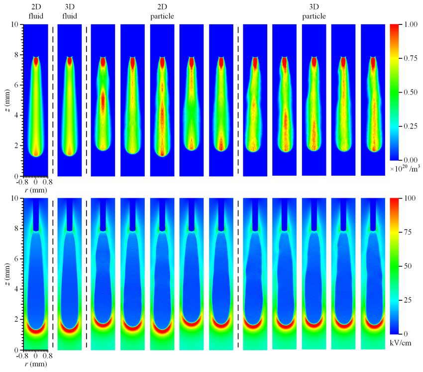
A comparison of particle and fluid models for positive streamer discharges in air                                   2

1. Introduction                                             Bulk coefficients describe the dynamics of a group
                                                            of electrons, whereas flux coefficients characterize the
Streamer discharges are elongated conducting channels       properties of individual electrons. Although the use
that typically appear when an insulating medium is          of flux coefficients is typically recommended [21, 22],
locally exposed to a field above its breakdown value [1].   it is not fully clear which type of data would give the
Electric field enhancement around their tips causes         best agreement between particle and fluid simulations
streamers to rapidly grow through electron impact           of positive streamers [1, 23]. Furthermore, with a two-
ionization. Due to this field enhancement, they can         term Boltzmann solver it possible to use either a spatial
propagate into regions in which the background field        or temporal growth model, which lead to different
was initially below breakdown. Streamers occur in           transport coefficients [24]. The second goal of this
nature as sprites [2, 3] and they are used in diverse       paper is therefore to determine the most suitable type
applications such as the production of radicals [4],        of transport data for use in fluid simulations of positive
pollution control [5], the treatment of liquids [6],        streamers.
plasma medicine [7], and plasma combustion [8].                   Past work Below, we briefly discuss some of
      Over the last decades, numerical simulations have     the past work on the comparison of particle and
become a powerful tool to study streamer physics            fluid models for streamer discharges. In [23], four
and to explain experimental results. Two types of           models were compared by simulating a short negative
models have commonly been used: particle models             streamer in 3D: a particle model, the ‘classical’ fluid
(e.g., [9–13]) and fluid models (e.g., [14–20]).            model with the local field approximation, an extended
      Particle models track the evolution of a large        fluid model, and a hybrid particle-fluid model. These
number of electrons, represented as (super-)particles,      simulations were carried out in a 1.2 mm gap using
and other relevant species. They can be used to study       a background electric field well above breakdown,
stochastic phenomena such as electron runaway or            without taking photoionization into account. The
discharge inception. Another advantage of such models       classical fluid model here deviated from the other
is that no assumptions on the EVDF (electron velocity       models in terms of streamer velocity and shape, but
distribution function) need to be made. In fluid models     this was probably due to an implementation flaw that
all relevant species are approximated by densities,         was later found. In [25] three plasma fluid models
which can greatly reduce computational costs. These         of different order were compared against particle
densities evolve due to fluxes and source terms, which      simulations for planar ionization waves, which can be
are computed by making certain assumptions about            thought of as “1D” negative streamers. The classical
the EVDF. Common is the local field approximation, in       fluid model was found to give rather reasonable results,
which it is assumed that electrons are instantaneously      somewhat in contrast with the conclusions of [26].
relaxed to the local electric field.                        Finally, in [27] six streamer codes from different
      Although both particle and fluid models have          groups were benchmarked against each other, aiming
frequently been used to study positive streamer             towards model verification. All codes implemented the
discharges, it is not clear how well these models agree.    classical fluid model, and three test cases with positive
The first goal of this paper is therefore to study the      streamers were considered. Good agreement was found
agreement between particle and fluid simulations of         on sufficiently fine grids, and with corresponding small
positive streamers in air, using both axisymmetric          time steps.
and 3D simulations. We use a standard particle                    Particle and fluid models have also been compared
model of the PIC-MCC (particle-in-cell, Monte Carlo         for other types of discharges. In [28] particle, fluid
collision) type and a standard drift-diffusion reactions    and hybrid models were benchmarked against each
fluid model with the local field approximation.             other and against experimental data. This review
      When comparing models, it is important to             paper focused on applications related to plasma display
have consistent input data computed from the same           panels, capacitively coupled plasmas and inductivetly
electron-neutral cross sections. However, transport         coupled plasmas. The authors conclude that “Excellent
coefficients for a fluid model can be computed with         agreement can be found in these systems when the
different types of Boltzmann solvers, and both so-          correct model is used for the simulation. Choosing
called flux and bulk coefficients can be computed.          the right model requires an understanding of the
A comparison of particle and fluid models for positive streamer discharges in air                                       3

capabilities and limitations of the models and of                                    1
                                                             ~v (t + ∆t) = ~v (t) +    [~a(t) + ~a(t + ∆t)] ,          (2)
the main physics governing a particular discharge.”.                                 2
Furthermore, in [29], particle and fluid models were          where ~a = −(e/me )E     ~ is the acceleration due to the
compared for capacitively and inductively coupled                            ~
                                                              electric field E, and e is the elementary charge and me
argon-oxygen plasmas, in [30] they were compared              the electron mass.
for atmospheric pressure helium microdischarges, and                In axisymmetric simulations particles are evolved
in [31] they were extensively compared for low-pressure       as in a 3D Cartesian geometry.               However, their
ccrf discharges.                                              acceleration, which is due to an axisymmetric field, is
     In contrast to the above work, we here compare           projected onto a radial and axial components before
multidimensional particle and fluid simulations of            it is used. The acceleration in equation (1) is then
positive streamers in air, propagating in background          given by ~a = (ar x/r, ar y/r, az ), where x and y denote
fields below breakdown, including photoionization.            the two (3D) particle coordinates       corresponding to the
The paper is organized as follows. In section 2, the                                          p
                                                              radial direction and r = x2 + y 2 . In equation (2),
particle and fluid models are described as well as the        the radial velocity is updated as
simulation conditions. In section 3.1, we first compare
                                                                                            1
axisymmetric and 3D particle and fluid simulations           ~vx,y (t + ∆t) = ~vx,y (t) + r̂ [ar (t) + ar (t + ∆t)] ,
of positive streamers in air, after which the influence                                     2
of transport data is studied with axisymmetric fluid          where r̂ = (x, y)/r.
simulations in section 3.2. We then investigate the                 Electron-neutral collisions are handled with the
numerical convergence of both types of models in              null-collision method [10, 33], using collision rates
section 3.3, and we determine the dominant source             calculated from cross section input data.
of stochastic fluctuations in the particle simulations in
section 3.4. Finally, in section 3.5, the models are again   2.1.2. Super-particles Due to the large number of
compared for different applied voltages.                     electrons in a streamer discharge, it is generally
                                                             not feasible to simulate all electrons individually.
2. Model description                                         Instead, so-called “super-particles” are used, whose
                                                             weights wi determine how many physical particles they
The particle and fluid models are briefly introduced         represent [34]. The procedure followed here is similar
below, after which the simulation conditions, photoion-      to that in [10]. A parameter Nppc controls the ‘desired’
ization and the adaptive mesh are described. We use          number of particles per grid cell. We use Nppc = 75,
both axisymmetric and 3D models. For brevity, ax-            except for section 3.4, in which it is varied. The desired
isymmetric models will sometimes be referred to as           particle weights ω are then determined as
“2D”.                                                        ω = ne × ∆V /Nppc                                        (3)
     Due to the short time scales considered in this
paper, ions are assumed to be immobile in both the           where ne is the electron density in a cell and ∆V
particle and fluid models. Information about the             the cell volume. Furthermore, the minimum particle
computational cost of simulations is given in Appendix       weight is ωmin = 1.
A.                                                                Particle weights are updated when the number of
                                                             simulations particles has grown by a factor of 1.25,
                                                             after the AMR mesh has changed, or after 10 time steps
2.1. Particle (PIC-MCC) model
                                                             in axisymmetric simulations (see below). The particles
We use a PIC-MCC (particle-in-cell, Monte-Carlo              in a cell for which wi < (2/3) × ω are merged, by
Collision) model that combines the particle model            combining two such particles that are close in energy
described in [10] with the Afivo AMR (adaptive mesh          into one with the sum of the original weights. The
refinement) framework described in [32]. Electrons are       coordinates and velocity of the merged particle are
tracked as particles, ions as densities, and neutrals        randomly selected from one of the original particles,
as a background that electrons stochastically collide        see [35]. Particles are split when wi > (3/2) × ω. Their
with. Below, we briefly introduce the model’s main           weight is then halved after which identical copies of
components.                                                  these particles are added, which will soon deviate from
                                                             them due to the random collisions.
 2.1.1. Particle mover and collisions The coordinates             In axisymmetric simulations particle weights are
~x and velocities ~v of simulated electrons are advanced     updated every ten time steps to reduce fluctuations
 with the ‘velocity Verlet’ scheme described in [10]:        near the axis. Figure 1 illustrates an axisymmetric
                                1                            mesh in which cell volumes depend on the radial
~x(t + ∆t) = ~x(t) + ∆t ~v (t) + ∆t2 ~a(t),           (1)    coordinate as ∆V = 2πr∆r∆z. Cells with small
                                2
                                                             volumes contain fewer physical electrons, and because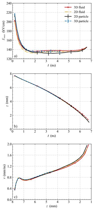
A comparison of particle and fluid models for positive streamer discharges in air                               4

                                                          these approaches are challenging to combine with the
                                                          cell-centered AMR used in our models.

                                                          2.1.4. Temporal discretization We use the following
                                                          CFL-like condition
                                                          ∆tcfl ṽmax ≤ 0.5 × ∆xmin ,                          (4)
                                                          where ∆xmin indicates the minimum grid spacing, and
                                                          ṽmax is an estimate of the particle velocity at the
                                                          90%-quantile. This prevents a few fast particles from
                                                          affecting ∆tcfl .
                                                               Another time step constraint is the Maxwell time,
                                                          also known as the dielectric relaxation time, which is a
                                                          typical time scale for electric screening:
                                                          ∆tdrt = ε0 / (ene,max µe ) ,                         (5)
                                                          where ε0 is the dielectric permittivity, ne,max is the
                                                          maximal electron density, and µe the electron mobility,
                                                          as determined in the local field approximation (see
                                                          section 2.2.2).
                                                               The actual time step is then the minimum of ∆tcfl
                                                          and ∆tdrt , and it is furthermore adjusted such that the
                                                          number of electrons does not grow by more than 20%
                                                          between time steps.

                                                          2.1.5. Input data We use Phelps’ cross sections for
                                                          N2 and O2 [37, 38]. These cross sections contain a
Figure 1: Illustration of the adaptive mesh in an         so-called effective momentum transfer cross sections,
axisymmetric streamer simulation, also showing the        which account for the combined effect of elastic and
electron density. The grid is coarser than in an actual   inelastic processes [39]. To use them in particle
simulation. The enlarged view illustrates the relation    simulations, we convert them to elastic cross sections
between cell volumes and radius.                          by subtracting the sum of the inelastic cross sections.
                                                          This is an approximate procedure, but the resulting
                                                          cross sections are suitable for a model comparison.
the minimal super-particle weight is one, stochastic
fluctuations in such cells are larger. Furthermore,       2.2. Fluid model
super-particle weights given by equation (3) are
                                                          We use a drift-diffusion-reaction fluid model with the
proportional to the cell volume. Particles with high
                                                          local field approximation, as implemented in [15]. The
weights can therefore cause significant fluctuations
                                                          electron density ne evolves in time as
when they move towards the axis.         We update
the particle weights more frequently in axisymmetric      ∂t ne = ∇ · (ne µe E + De ∇ne ) + SR + Sph          (6)
simulations to limit these fluctuations.                  where µe and De indicate the electron mobility
                                                          and the diffusion coefficient, Sph is the non-local
2.1.3. Mapping particles to the grid Particles are        photoionization source term (see section 2.4), and SR
mapped to grid densities using a standard bilinear or     is a source term due to the following ionization and
trilinear weighting scheme, as in [10]. Near refinement   attachment reactions:
boundaries, the mapping is locally changed to the         e + N2 −→ 2e + N+    2 (15.60 eV)
“nearest grid point” (NGP) scheme, to ensure that         e + N2 −→ 2e + N+    2 (18.80 eV)
particle densities are conserved. In axisymmetric
coordinates the mapping is also done using bilinear       e + O2 −→ 2e + O+
                                                                          2
weighting, but the radial variation in cell volumes is    e + 2O2 −→ O−
                                                                      2 + O2
taken into account. The interpolation of the electric     e + O2 −→ O− + O
field from the grid to particles is done using standard   Ion densities also change due to the above reactions.
bilinear (2D) or trilinear (3D) interpolation. Note       Transport coefficients and reaction rates are deter-
that there are more advanced weighting schemes for        mined using the local field approximation, see section
handling axisymmetric coordinates systems [36], but       2.2.2.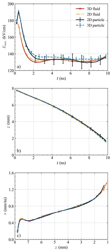
A comparison of particle and fluid models for positive streamer discharges in air                                   5

2.2.1. Time integration Advective electron fluxes are       This electrode is 2.0 mm long and has a radius of 0.2
computed using the Koren flux limiter [40] and diffusive    mm.
fluxes using central differences, see [15] for details.           For the electric potential, Dirichlet boundary
Time integration is performed with Heun’s method,           conditions are applied to the lower and upper domain
a second order accurate explicit Runge-Kutta scheme.        boundaries, and a homogeneous Neumann boundary
Time steps are limited according to the following           condition is applied on the other boundaries. In terms
restrictions:                                               of electrostatics the axisymmetric and 3D simulations
                                                            are not fully equivalent, because of the different

        2Ndim X vi
∆tcfl          +            ≤ 0.5,                          geometry in which these boundary conditions are
         ∆x2           ∆x
                                                            applied.
∆tdrt (ene µe /ε0 ) ≤ 1,
                                                                  For the electron density homogeneous Neumann
∆t = 0.9 × min(∆tdrt , ∆tcfl ),                             conditions are applied on all domain boundaries,
where ∆tcfl corresponds to a CFL condition (includ-         except for the rod electrode. The electrode absorbs
ing diffusion), ∆tdrt corresponds to the dielectric re-     electrons but does not emit them. Since a positive
laxation time (as in equation (5)), Ndim is the dimen-      voltage is applied on this electrode, secondary electron
sionality of the simulation, ∆t is the actual time step     emission was not taken into account.
used, and ∆x stands for the grid spacing, which is here           There is initially no background ionization besides
equal in all directions.                                    an electrically neutral plasma seed that is placed at the
                                                            tip of the electrode. This seeds helps to start discharges
2.2.2. Input data The fluid model requires tables           in almost the same way in particle and fluid models.
of transport and reaction data versus electric field        The electron and positive ion densities are given by a
strength as input. We use two methods to compute            Gaussian distribution:
                                                                                               (r − r0 )2

such data from the cross sections that were also used                            16 −3
                                                            ni (r) = ne (r) = 10 m exp                      ,      (7)
for the PIC model, see section 2.1.5. The first is                                            (0.1 mm)2
BOLSIG+, which is a widely used two-term Boltzmann          where r0 is the location of the tip of the electrode,
solver [24, 41]. When the electron velocity distribution    which is at z ≈ 7.8 mm.
is strongly anisotropic, for example in high electric            In particle simulations, these initial densities are
fields, the use of the two term approximation can           converted to N = bne ∆V c simulation particles per cell,
introduce errors [42]. The second method we use is          each with a weight of one. A uniform [0, 1) random
a Monte Carlo swarm code gitlab.com/MD-CWI-NL/              number is compared to the remainder to determine
particle_swarm, similar to e.g. [43, 44]. The basic         whether to add one more particle. The goal of this
idea of this approach is to trace electrons in a uniform    sampling is to reduce stochastic fluctuations in the
field, from which transport and reactions coefficients      initial conditions. The initial particles are spread
can be obtained.                                            uniformly within each grid cell, and they initially have
      With the Monte Carlo method we compute both           zero kinetic energy.
so-called flux and bulk coefficients [22]. Flux data
describes the average properties of individual electrons,
                                                            2.4. Photoionization
whereas bulk data describes average properties of a
group of electrons, taking ionization and attachment        For streamers in air, photoionization is typically the
processes into account. One of the main differences is      main source of free electrons. The process results from
that in high fields the bulk mobility is higher than the    the interaction between an oxygen molecule and an UV
flux mobility, as shown in figure 5. Unless mentioned       photon emitted from an excited nitrogen molecule. We
otherwise, the fluid simulations presented in this paper    use Zheleznyak’s model for photoionization in air [45]
use Monte Carlo flux data.                                  and compute photoionization as in [17]. Assuming
                                                            that ionizing photons do not scatter and their direction
2.3. Computational domain and initial conditions            is isotropically distributed, the photoionization source
                                                            term in equation (6) is given by:
Simulations are performed in artificial air, containing
                                                                          I(r0 )f (|r − r0 |) 3 0
                                                                      Z
80% N2 and 20% O2 , at p = 1 bar and T = 300 K.             Sph (r) =                    2 d r ,                 (8)
The computational domain used for the comparison of                         4π |r − r0 |
cylindrical models is shown in figure 2. It measures 10     where f (r) is the photon absorption function and I(r)
mm in both the axial and radial directions. For the 3D      is the source of ionizing photons, which is proportional
Cartesian simulations, a similar domain of 20 mm ×          to the electron impact ionization source term Si :
20 mm × 10 mm is used. A rod-shaped electrode with                    pq
a semi-spherical cap is placed at center of the domain.     I(r) =         ξSi ,                                 (9)
                                                                    p + pq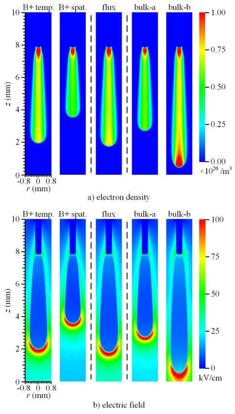
A comparison of particle and fluid models for positive streamer discharges in air 6
2.5. Afivo AMR framework
The open-source Afivo framework [32] is used in
both particle and fluid models to provide adaptive
mesh refinment (AMR) and a parallel multigrid
solver. Adaptive mesh refinement (AMR) is used
for computational efficiency, based on the following
criteria [15]:
• refine if α(E)∆x > c0 ,
• de-refine if α(E)∆x < 0.125c0 , but only if ∆x is
smaller than 10 µm.
Here ∆x is the grid spacing, which is equal in
all directions, α(E) is the field-dependent ionization
coefficient, and c0 is a constant. Furthermore, the
grid spacing is bound by ∆x ≤ 0.4 mm. For 3D
particle simulations we use c0 = 1.0 and for all other
simulations c0 = 0.8. Slightly less refinement is used
for the 3D particle simulations because of their large
Figure 2: Schematic view of the axisymmetric computational cost, see Appendix A. With these values
computational domain used for both particle and fluid for c0 numerical convergence errors are reasonably
models, showing the initial electron density and the small, as discussed in section 3.3.
electrode. 3D simulations are performed in a similarly The geometric multigrid solver in Afivo [32] is used
sized domain, measuring 20 mm × 20 mm × 10 mm. to efficiently solve Poisson’s equation ∇2 φ = ρ/ε0 ,
where φ is the electric potential, ε0 the permittivity of
vacuum and ρ the space charge density. Electrostatic
where p is the gas pressure, pq = 40 mbar is a fields are then computed as E ~ = −∇φ. The same
quenching pressure. For simplicity, we use a constant type of multigrid solver is also used to solve the
proportionality factor ξ = 0.075, except for section 3.4, Helmholtz equations for photoionization. To include
in which ξ is varied. a needle electrode, we set the applied potential as
We solve equation (8) in two ways in this paper. a boundary condition at the electrode surface. This
For fluid simulations, we use the so-called Helmholtz was implemented by modifying the multigrid methods
expansion [46, 47]. By approximating the absorption using a level-set function.
function, the integral in equation (8) can be turned
into multiple Helmholtz equations that can be solved
3. Results
by fast elliptic solvers. We use Bourdon’s three-term
expansion, as described in [46] and appendix A of [27]. 3.1. Axisymmetric and 3D results
For particle simulations, we use a discrete Monte
Carlo photoionization model as described in [17, 48]. In this section, we compare axisymmetric and 3D
With this model stochastic effects due to discrete particle and fluid models, using the computational
single photons are simulated. The basic idea is to configuration and initial condition described in section
stochastically sample the generated photons, their 2.3. A voltage of φ = 11.70 kV is applied, which results
directions, and their travel distances. We also use in a background field of around 15 kV/cm; about half
this approach for the fluid simulations in section 3.4, the breakdown field of air.
see [17] and chapter 11 of [49] for details. Photoionization in the fluid model is here
These two approaches for photoionization differ computed with the Helmholtz approximation, whereas
not only in terms of stochastic effects. Because of the the particle model uses a Monte Carlo scheme
way the absorption function is approximated in the with discrete photons. To account for stochastic
Helmholtz approach, the number of ionizing photons fluctuations, ten runs of the 2D cylindrical and 3D
produced and their absorption profile will also be particle models are performed, of which five are shown.
somewhat different. However, such small differences For the fluid simulations flux transport data from
in photoionization usually have only a minor effect on Monte Carlo swarms is used, see section 2.2.2.
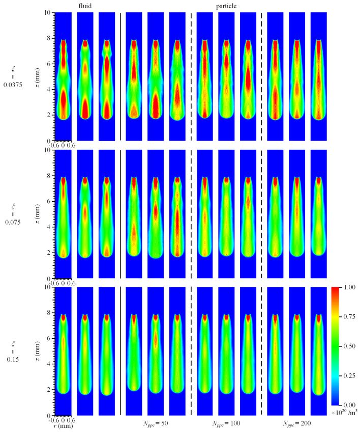
discharge development, as confirmed by our results in Figure 3 shows the electron densities and electric
section 3. fields for the different models at t = 10 ns. The
electric field and electron density profiles are similar
for all cases, and the streamer head positions are in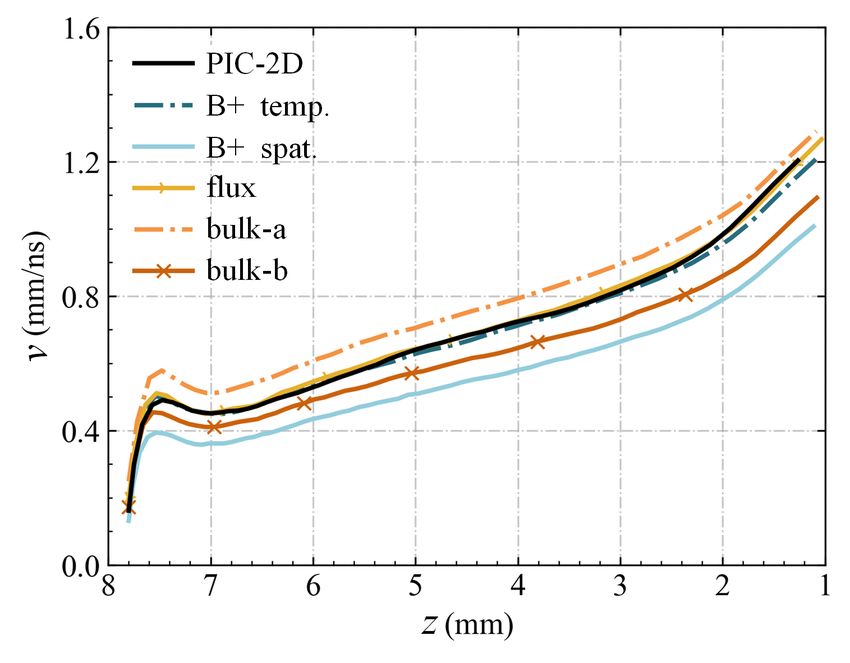
A comparison of particle and fluid models for positive streamer discharges in air                                  7

Figure 3: The electron densities and electric fields at t = 10 ns for fluid and particle models at an applied voltage
of 11.70 kV. The axisymmetric results are mirrored in the symmetry axis. For the 3D simulations cross sections
are shown. Multiple runs are shown for the stochastic particle simulations. For the fluid simulations Monte
Carlo flux transport data was used.

good agreement, with deviations in streamer length          of super-particles. This is computationally not feasible
below 5%. Streamer head positions in all models at          for the simulations performed here.
t = 3, 6, 9 ns are given in table 1.                             Stochastic fluctuations are not present in the fluid
     With the axisymmetric particle model stochastic        simulations, in which the electron densities and electric
fluctuations are visible in the streamer radius and the     fields evolve smoothly in time. The results of the
electron densities. As discussed in section 3.4 this is     cylindrical and 3D fluid models are nearly identical.
mainly due to the stochastic photoionization used in        Small differences can occur because the computational
the particle simulations. Streamers appear to prop-         domains correspond to a rectangle and a cylinder,
agate somewhat slower due to these fluctuations. In         which means that the applied boundary conditions
3D similar fluctuations are present, but the stream-        are not equivalent. Furthermore, the numerical grids
ers can now move slightly off axis. The 3D particle         and operators are also slightly different in these two
model can in principle capture realistic stochastic fluc-   geometries.
tuations, but only if single electrons are used instead          To more quantitatively analyze the differences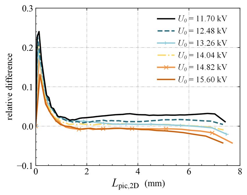
A comparison of particle and fluid models for positive streamer discharges in air                                8

                                                           Model      Data          z (3 ns)   z (6 ns)   z (9 ns)
                                                           PIC-2D     -             6.45       4.74       2.41
                                                           PIC-3D     -             6.45       4.71       2.39
                                                           fluid-2D   flux          6.40       4.64       2.31
                                                           fluid-3D   flux          6.42       4.66       2.35
                                                           fluid-2D   B+ temp.      6.42       4.71       2.47
                                                           fluid-2D   B+ spat.      6.72       5.46       3.87
                                                           fluid-2D   bulk-a        6.19       4.13       1.34
                                                           fluid-2D   bulk-b        6.54       5.04       3.12

                                                          Table 1: Streamer head position (z, in mm) at 3, 6 and
                                                          9 ns in different simulations, using an applied voltage
                                                          of 11.7 kV. The bottom part of the table gives results
                                                          for different types of transport data, see section 3.2.
                                                          Here “B+ (temp.)” and “B+ (spat.)” respectively refer
                                                          to flux data computed with BOLSIG+ using temporal
                                                          growth and spatial growth models, and “bulk(a)” and
                                                          “bulk(b)” refer to two types of bulk coefficients.

                                                          between models, the maximal field Emax , the streamer
                                                          head position z and streamer velocity v are shown in
                                                          figure 4. The streamer head position is defined as the
                                                          z-coordinate where the electric field is maximal. The
                                                          velocity is shown versus streamer position, otherwise
                                                          initial differences grow larger over time even if models
                                                          agree well later on. The streamer velocity is computed
                                                          as the numerical derivative of the streamer head
                                                          position, which amplifies fluctuations. We use a
                                                          Savitzky–Golay filter of width 5 and order 2 to compute
                                                          a smoothed velocity from the position versus time data.
                                                          For the stochastic particle simulations the average of
                                                          ten runs is shown.
                                                               The maximal electric field follows a similar trend
                                                          in all models, with first a field of about 180 kV/cm
                                                          and then a relaxation towards a field of about 130–
                                                          135 kV/cm as the streamers propagate across the gap.
                                                          When the streamers approach the grounded electrode
                                                          the maximal field increases again, because the available
                                                          voltage difference is compressed in a small region.
                                                               The peak electric fields during inception differ
                                                          somewhat, with the particle model having the highest
                                                          peak at about 190 kV/cm whereas it is about 180
                                                          kV/cm for both fluid models. The relaxation of this
                                                          peak electric field occurs about 0.4 ns earlier in the
Figure 4: Comparison between axisymmetric and 3D          fluid model. The main reason for this is that near
particle and fluid simulations at an applied voltage      the electrode, the degree of ionization in the streamer
of 11.70 kV. From top to bottom: maximal electric         channel is somewhat higher in the particle simulations,
field versus time, streamer head position versus time     which initially leads to stronger field enhancement.
and front velocity versus streamer position. For the           For this study, we have designed the initial
stochastic particle simulations the average of ten runs   conditions such that inception behavior would be
is shown, and the error bars indicate ± one standard      similar in the particle and fluid simulations, by using
deviation.                                                a sharp electrode and a compact initial seed with
                                                          sufficiently many electrons. If we define inception as
                                                          the moment at which the streamer crosses the position
                                                          z = 7.6 mm, then inception is about 0.04 ns faster in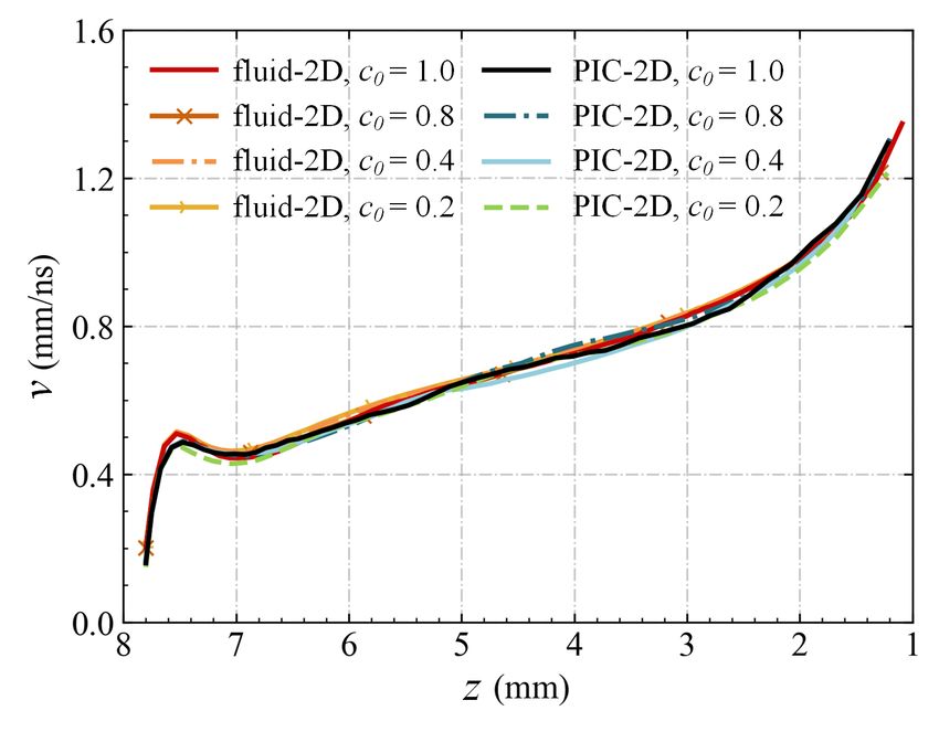
A comparison of particle and fluid models for positive streamer discharges in air                                    9

the fluid simulations. This could be due to the local         • (flux) Flux data computed with a Monte
field approximation, with which electrons are assumed           Carlo swarm method (available at gitlab.com/
to instantaneously relax to the background electric             MD-CWI-NL/particle_swarm), which uses the
field. Electron multiplication therefore happens more           same core routines for simulating electrons as our
rapidly in the fluid simulations at t = 0 ns, and               particle model [10].
similarly photoelectrons also instantaneously produce         • (bulk-a) Bulk data computed with the same
new ionization. We remark that when inception is                Monte Carlo swarm method. In this variant,
highly stochastic (with different initial conditions),          only the transport terms in equation (6) are
another difference could be more relevant. With a fluid         modified, by computing the electron flux as
model low densities always rapidly grow in a high field,        −ne µB        B             B        B
                                                                      e E−De ∇ne , where µe and De denote bulk
even if they correspond to a small probability of an            coefficients.
electron being present, as was observed in [50]. Such
                                                              • (bulk-b) The same bulk data as above, but in this
continuous growth of a low electron density in high field
                                                                variant the reaction terms in equation (6) are also
regions can then lead to faster inception.
                                                                modified by multiplying them with µB  e /µe , where
      There is good agreement among the models for
                                                                µe denotes the standard flux mobility.
the streamer position versus time, and thus also for the
streamer velocities as a function of streamer position.     With the bulk-a approach reaction rates are the same
Velocity differences are generally less than 0.04 mm/ns     as with flux data. However, the number of reactions
among the models. The mean relative deviation in            taking place per unit length (traveled by electrons) is
velocity is below 2%. We compute this quantity as           changed, i.e., the so-called Townsend coefficients are
Z                       Z                                  different. With the bulk-b approach it is the other
    |va (z) − vb (z)|dz    va (z)dz ,               (10)    way around.
                                                                 Different types of transport data are shown in
where va and vb denote the velocities in the particle       figure 5. Above about 180 Td ionization becomes
and fluid simulations, which are linearly interpolated      important and bulk mobilities are larger than flux
between known positions. After inception velocities         mobilities. The spatial growth model of BOLSIG+
increase approximately linearly with streamer length.       leads to a significantly smaller ionization coefficient. In
At the end of the gap they increase more rapidly due        high electric fields, its value is about 25-30% less than
to boundary effects.                                        that of the other approaches. With the Monte Carlo
                                                            approach both transverse and longitudinal diffusion
3.2. Fluid model transport and reaction data                coefficients are computed, but in our fluid simulations
                                                            we for simplicity only use the transverse ones. The
As mentioned in section 2.2.2, transport and reaction
                                                            BOLSIG+ flux diffusion coefficient also corresponds
data for a fluid model can be computed using different
                                                            to the transverse direction [24, 39], but it is larger
types of Boltzmann solvers. Furthermore, both so-
                                                            than the Monte Carlo flux coefficient. Such differences
called flux and bulk data can be computed. Flux data
                                                            between diffusion coefficients computed with a two-
describes the behavior of individual electrons, whereas
                                                            term approach and higher-order methods have been
bulk data describes the behavior of a group of electrons,
                                                            observed before, see e.g. [51]. However, the different
taking ionization and attachment into account. We
                                                            diffusion coefficients only have a minor impact on our
here study how the choice of fluid model input data
                                                            simulations, as shown below.
affects the the consistency between particle and fluid
                                                                 Figure 6 shows axisymmetric fluid simulations
simulations. The following types of input data are
                                                            with the input data listed above; streamer positions
considered (with labels in bold):
                                                            over time are given in table 1 and streamer velocities
  • (B+ temp.)         Flux data computed with              in figure 7. There are minor differences in streamer
    BOLSIG+ using its temporal growth model [24].           velocity when comparing the BOLSIG+ flux data
    With this setting, the two-term approximation           with temporal growth and the Monte Carlo flux
    is solved by assuming that the electron density         data. When comparing streamer velocities at the same
    grows exponentially in time. This is the default        length, relative differences are below 3%. With both
    growth model, but it is not clear whether it            types of data good agreement is obtained with the
    is the most suitable growth model for streamer          axisymmetric particle simulations. In contrast, the
    simulations [24].                                       BOLSIG+ data with the spatial growth model leads
  • (B+ spat.) Flux data computed with BOLSIG+              to a streamer velocity that is much too low, due to the
    using its spatial growth model [24], in which           lower ionization coefficient.
    it is assumed that the electron density grows                Both types of bulk transport data lead to
    exponentially in space.                                 significant deviations compared to the particle model.
                                                            When only the transport coefficients are changed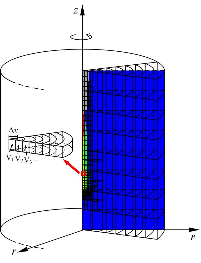
A comparison of particle and fluid models for positive streamer discharges in air                                   10

Figure 5: Different types of electron transport coefficients computed for 80% N2 and 20% O2 at p = 1 bar and T
= 300 K, using Phelp’s cross sections, see section 2.1.5. For BOLSIG+ data is shown using both a temporal and
a spatial growth model. The data labeled “bulk” and “flux” was computed with a Monte Carlo swarm code. Both
transverse and longitudinal diffusion coefficients were computed with this technique, but only the transverse
coefficients are used in our fluid model.

(bulk-a), the streamer is significantly slower and it has    3.3. Mesh refinement and numerical convergence
a lower degree of ionization. With this data electrons
                                                             We here study the sensitivity of the particle and fluid
drift faster, but the degree of ionization produced in the
                                                             simulations to the grid spacing, to test whether our
streamer channel is lower, leading to a slower discharge.
                                                             simulations are close to numerical convergence. To
However, when the reaction terms are also changed
                                                             control the grid spacing, the refinement parameter c0
(bulk-b), the streamer propagates too fast. The higher
                                                             is varied, see section 2.5. Note that the time step in
streamer velocity is to be expected, since most terms
                                                             both models will also be affected by the grid spacing,
on the right-hand side of equation (6) are now scaled
                                                             as explained in section 2.1.4 and 2.2.1.
with the bulk mobility.
                                                                  Figure 8 shows streamer velocities versus streamer
     In conclusion, bulk data and data computed with
                                                             position for c0 values of 1.0, 0.8, 0.4 and 0.2, for which
a spatial growth model are not recommended for the
                                                             the minimal grid spacing is 3.9, 3.9, 1.9, and 0.9 µm,
simulation of positive streamers. With flux transport
                                                             respectively. Streamer positions at t = 3, 6 and 9 ns
data there are minor differences between BOLSIG+
                                                             are given in table 2. With the fluid model, deviations
data computed with a temporal growth model and
                                                             in length at t = 9 ns are about 3% with c0 = 0.8
Monte Carlo data, but both lead to good agreement
                                                             compared to the finest-grid case. With the particle
with the particle simulations.
                                                             model, there are statistical fluctuations that make it
                                                             harder to establish numerical convergence, but at t = 9
A comparison of particle and fluid models for positive streamer discharges in air 11
Figure 7: Streamer velocity versus streamer head
position for different types of transport data. The
labels are explained in figure 6 and in section 3.2.
Figure 6: Electron densities and electric fields at t = 9.6
ns for axisymmetric fluid simulations with an applied Figure 8: Streamer front velocities versus streamer
voltage of 11.7 kV. Different types of transport data head position for different refinement criteria. Other
are used, from left to right: BOLSIG+ with temporal conditions are the same as in section 3.1. For the
growth, BOLSIG+ with spatial growth, Monte Carlo particle simulations the average of ten runs is shown
flux data, and two types of Monte Carlo bulk data. to reduce stochastic fluctuations.
With bulk-a only transport terms are modified, and
with bulk-b reaction terms are also scaled with the bulk
mobility. ns streamer lengths are also within 3% for all tested
cases. When comparing the streamer velocity versus
position for c0 = 0.8 and c0 = 0.2, convergence errors
are about 1% for the fluid model and about 2% for the
particle model, using equation (10).
Table 2 allows to compare differences in streamer
length between particle and fluid simulations using
the same refinement. Interestingly, these differences
are larger on finer grids: with c0 = 0.2, the relative
differences in streamer length are about 8–10% at 3, 6
and 9 ns, whereas for c0 = 0.8 they are about 2–4%.
For streamer velocities (compared at the same streamerA comparison of particle and fluid models for positive streamer discharges in air 12
Model c0 z (3 ns) z (6 ns) z (9 ns) particles per cell in particle simulations, see equation
PIC-2D 0.2 6.51 4.81 2.59 3.
±0.02 ±0.09 ±0.11 Figure 9 shows results of axisymmetric particle
PIC-2D 0.4 6.45 4.74 2.54 and fluid models for ξ = 0.0375, 0.075, 0.15 and Nppc
±0.03 ±0.04 ±0.06 = 50, 100, 200. In both models the streamer length
PIC-2D 0.8 6.45 4.74 2.41 is not sensitive to the amount of photoionization, as
±0.03 ±0.11 ±0.21 was also observed in e.g. [52]. However, fluctuations
PIC-2D 1.0 6.45 4.71 2.45 in the electron density are significantly larger for the ξ
±0.04 ±0.13 ±0.13 = 0.0375 case, whereas these fluctuations are reduced
fluid-2D 0.2 6.37 4.54 2.14 for the ξ = 0.15 case, as was also observed in [17].
fluid-2D 0.4 6.37 4.55 2.17 With ξ = 0.0375 we even observed branching in a
fluid-2D 0.8 6.40 4.64 2.31 few of the simulation runs, which is probably due to
fluid-2D 1.0 6.42 4.67 2.35 increased density fluctuations near the z-axis when the
amount of photoionization is decreased. Fluctuations
Table 2: Streamer head position (z, in mm) at 3, 6 in the streamer radius are also larger for a lower
and 9 ns, using an applied voltage of 11.7 kV. Different value of ξ. When Nppc is increased, fluctuations
values of the refinement parameter c0 are used, see in electron densities and streamer radius are slightly
section 2.5. For the particle simulations averages reduced, but the effect is weaker than that of the ξ
over ten runs are shown, together with the standard parameter. We therefore conclude that the discrete
deviation of the sample. Streamer lengths are given by photoionization model is responsible for most of the
7.8 mm − z. stochastic fluctuations in our results. This confirms
the assumptions made in recent work [17, 53], in which
fluid models were used to demonstrate the importance
length) the mean deviations are about 4% and 2% for
of stochastic photoionization on streamer branching.
these two cases, using equation (10).
Finally, we remark that in figure 9 the stochastic
Based on the above, we conclude that numerical
fluctuations are demonstrated with axisymmetric
convergence errors are relatively small for our default
models, in which these fluctuations are not completely
refinement parameter c0 = 0.8 – they do at least not
physical. We have also performed 3D fluid simulations
exceed the intrinsic differences between the models,
with stochastic photoionization, in which these
which are already quite small. For the test case
fluctuations looked qualitatively similar to those shown
considered here, with an applied voltage of 11.7 kV, the
in figure 3 for the 3D particle model. However,
difference in streamer velocity is about twice as large
a statistical comparison of these 3D models for the
(4% instead of 2%) on the finest grid. The main reason
parameter range shown in figure 9 could not be
for this is that in the fluid simulations, which are more
performed due to the high computational costs of the
sensitive to the grid refinement, the streamer velocity is
3D particle simulations.
somewhat higher on finer grids. In section 3.5 we show
that for higher applied voltages, the velocity is actually
higher in the particle simulations. We therefore expect 3.5. Results at different voltages
that using a finer grid somewhat increases model Figure 10 shows results for particle and fluid
discrepancies for lower applied voltages, and that simulations at a higher applied voltage of 14.04 kV,
is somewhat reduces model discrepancies for higher which results in a background electric field of about 18
applied voltages. kV/cm. All the other parameters are the same as in
section 3.1. For the 3D particle model results at later
3.4. Stochastic fluctuations times are missing, because these simulations exceeded
the memory and time constraints of our computational
To investigate the source of stochastic fluctuations in
hardware, see Appendix A.
the axisymmetric simulations we vary two parameters.
At this higher voltage, the agreement between the
The first is the photoionization factor ξ, see equation
models is of similar quality as in figure 4, but there are
9, which is a proportionality factor that relates the
a few differences. Figure 10(a) shows that inception is
number of UV photons produced to the electron
significantly faster. The relaxation of the initial high
impact ionization source term. It therefore directly
field takes place in about 1 ns, so roughly twice as fast,
controls the amount of photoionization. To study
and the curves for the maximal electric field are now
how ξ affects stochastic behavior, we use the discrete
in better agreement. With a higher applied voltage
photoionization model in both the particle and the fluid
the streamer velocity is higher, but the propagation is
simulations presented here. The second parameter we
otherwise similar to that in figure 4. The agreement
vary is Nppc , which controls the ‘desired’ number of
between the models is still good: between the 2DA comparison of particle and fluid models for positive streamer discharges in air 13 Figure 9: Electron densities at t = 10 ns in axisymmetric fluid and particle simulations. The photoionization coefficient ξ and the desired number of particles per cell Nppc are varied. For each combination of two parameters, three runs are shown. Stochastic photoionization is now also used in the fluid model. The condition are otherwise the same as in section 3.1.
A comparison of particle and fluid models for positive streamer discharges in air                                14

particle and 2D fluid simulations, the mean deviation
in velocity (compared at the same streamer length)
is about 1%. However, the discrepancy between the
2D and 3D fluid simulations is now somewhat larger.
This is probably due to the difference in computational
domains and electrostatic boundary conditions in 2D
and 3D, which could play a stronger role for a more
conducting streamer channel at a higher voltage. The
sensitivity of discharge simulations to these boundary
conditions was recently observed in [50].
     Figure 11 shows the relative difference ∆L in
streamer length between axisymmetric particle and
fluid models for applied voltages from 11.70 kV to
15.60 kV. These voltages correspond to background
electric fields of about 15 kV/cm to 20 kV/cm. The
difference is computed as
∆L = (Lfluid,2D − Lpic,2D )/Lpic,2D ,
where Lfluid,2D and Lpic,2D are the streamer lengths in
the fluid and particle model at a particular time.
     In all cases, ∆L peaks during streamer inception.
This happens because inception occurs faster in the
fluid model, as explained in section 3.1, and because
the denominator is initially small. For higher applied
voltages, the initial peak in ∆L becomes smaller.
     In which model the streamer has advanced the
furthest at a particular time depends on the applied
voltage.     When U0 is lower than 14.04 kV, ∆L
is generally positive, whereas for higher voltages it
becomes negative. This indicates that relative to
the fluid simulations, the velocity in the particle
simulations is higher at higher voltages. The mean
deviations between velocities in the particle and fluid
simulations are 1.8% (11.7 kV case), 1.9% (12.48 kV),
1.3% (13.26 kV), 1.3% (14.04 kV), 1.4% (14.82 kV) and
2.4% (15.6 kV).

4. Conclusions

We have quantitatively compared a PIC-MCC
(particle-in-cell, Monte Carlo collision) model and a
drift-diffusion-reaction fluid model with the local field
approximation for simulating positive streamer dis-
charges. The simulations were performed in air at 1
bar and 300 K, in background fields below breakdown
ranging from 15 kV/cm to 20 kV/cm, using both ax-           Figure 10: Comparison between axisymmetric and 3D
isymmetric and fully three-dimensional geometries.          particle and fluid models at an applied voltage of 14.04
     We have found surprisingly good agreement              kV, similar to figure 4. From top to bottom: the
between the particle and fluid simulations. Streamer        maximal electric field and streamer position versus
properties such as maximal field, radius, and velocity      time, and streamer velocity versus streamer position.
were all very similar. When compared at the same            For the particle model the average of ten runs is shown
streamer length, the mean difference in streamer            with error bars indicating ± one standard derivation.
velocity was generally below 4%. One source of
differences was the photoionization model, for which we
used a stochastic approach in the particle simulations
A comparison of particle and fluid models for positive streamer discharges in air 15
• Stochastic fluctuations are visible in axisymmetric
and 3D particle simulations, for example in the
streamer’s degree of ionization, maximal electric
field and radius. In our simulations, the dominant
source of these stochastic fluctuations is discrete
photoionization. Fluid simulations with the same
discrete photoionization model exhibit similar
fluctuations as particle simulations. Due to
these fluctuations, streamers in 3D simulations
propagate slightly off-axis. In the particle
simulations, the number of particles per cell did
not significantly affect these fluctuations.
• Axisymmetric simulations were performed for
applied voltages between 11.7 kV to 15.6 kV,
corresponding to background fields of about 15
kV/cm to 20 kV/cm. Discrepancies in streamer
Figure 11: The relative difference ∆L in streamer length (versus time) between particle and fluid
length versus time, shown for axisymmetric particle simulations were generally below 3%. The mean
and fluid simulations at several voltages. The differ- deviations in streamer velocity (versus length)
ence is computed as ∆L = (Lfluid,2D − Lpic,2D )/Lpic,2D . were about 2% for all applied voltages. Other
Besides the applied voltage, simulations conditions are streamer properties, such as the maximal electric
the same as in section 3.1. field, were also in good agreement.
Acknowledgments
and a continuum approach in most of the fluid
simulations. Part of this work was carried out on the Dutch
We have investigated the effect of different types national e-infrastructure with the support of SURF
of transport data in fluid models, how well the models Cooperative. This work was partly funded by
are numerically converged, what the main source of the China Scholarship Council (CSC) (Grant No.
stochastic fluctuations is, and how the agreement 202006280465). This work was supported by the
between the models is affected by the applied voltage. National Natural Science Foundation of China (Grant
Our main conclusions on these topics are: No. 51777164).
• The type of transport data used in a fluid model
is important. By using flux transport coefficients Data availability statement
computed with a Monte Carlo approach or
BOLSIG+ (using its temporal growth model), The data that support the findings of this study are
good agreement is obtained between the fluid openly available at the following URL/DOI: https:
and particle simulations. The use of bulk //doi.org/10.5281/zenodo.5509678.
coefficients leads to either faster or slower streamer
propagation, depending on how the coefficients are Appendix A. Computational hardware and
used. Data computed with the spatial growth costs
model of BOLSIG+ leads to a significantly slower
streamer discharge. Typical computing times for the results in section
• Numerical convergence errors are small in the 3.1 were a few minutes (2D fluid model), 8h (3D
particle and fluid simulations presented here. fluid model), and 2-3h (2D particle model). These
We have compared axisymmetric particle and computations ran on an Intel(R) Core(TM) i9-9900K
fluid simulations with grid refinement satisfying eight-core processor, using OpenMP parallelization.
α(E)∆x < c0 for c0 = 0.2, 0.4, 0.8 and 1.0, where The 3D particle simulations were performed on
α(E) is the ionization coefficient. For an applied Cartesius, the Dutch national supercomputer. A single
voltage of 11.7 kV, convergence errors in streamer thin node with a Intel Xeon E5-2690 v3 (Haswell)
velocity (compared at the same position) were 24-core processor and 64 GB of RAM was used.
about 1% for the fluid simulations and about 2% Computations ran for up to five days, with up to 600
for the particle simulations. On the finest grids, million particles.
streamer velocities increased slightly in the fluid
simulations.A comparison of particle and fluid models for positive streamer discharges in air 16
References emission. Plasma Sources Science and Technology,
25(4):044008, July 2016.
. [15] Jannis Teunissen and Ute Ebert. Simulating streamer
[1] Sander Nijdam, Jannis Teunissen, and Ute Ebert. The discharges in 3d with the parallel adaptive afivo
physics of streamer discharge phenomena. Plasma framework. Journal of Physics D: Applied Physics,
Sources Science and Technology, 29(10):103001, 2020. 50(47):474001, 2017.
[2] Ute Ebert, Sander Nijdam, Chao Li, Alejandro Luque, [16] J-M Plewa, O Eichwald, O Ducasse, P Dessante, C Jacobs,
Tanja Briels, and Eddie van Veldhuizen. Review of N Renon, and M Yousfi. 3D streamers simulation in
recent results on streamer discharges and discussion of a pin to plane configuration using massively parallel
their relevance for sprites and lightning. Journal of computing. Journal of Physics D: Applied Physics,
Geophysical Research: Space Physics, 115(A7), 2010. 51(9):095206, March 2018.
[3] Victor P. Pasko, Jianqi Qin, and Sebastien Celestin. To- [17] Behnaz Bagheri and Jannis Teunissen. The effect of
ward Better Understanding of Sprite Streamers: Initia- the stochasticity of photoionization on 3d streamer
tion, Morphology, and Polarity Asymmetry. Surveys in simulations. Plasma Sources Science and Technology,
Geophysics, 34(6):797–830, November 2013. 28(4):045013, 2019.
[4] Seiji Kanazawa, Hirokazu Kawano, Satoshi Watan- [18] Robert Marskar. An adaptive Cartesian embedded
abe, Takashi Furuki, Shuichi Akamine, Ryuta Ichiki, boundary approach for fluid simulations of two- and
Toshikazu Ohkubo, Marek Kocik, and Jerzy Mizeraczyk. three-dimensional low temperature plasma filaments in
Observation of oh radicals produced by pulsed discharges complex geometries. Journal of Computational Physics,
on the surface of a liquid. Plasma Sources Science and 388:624–654, July 2019.
Technology, 20(3):034010, 2011. [19] A Yu Starikovskiy and N L Aleksandrov. How pulse
[5] Hyun-Ha Kim. Nonthermal Plasma Processing for Air- polarity and photoionization control streamer discharge
Pollution Control: A Historical Review, Current Issues, development in long air gaps. Plasma Sources Science
and Future Prospects. Plasma Processes and Polymers, and Technology, 29(7):075004, July 2020.
1(2):91–110, September 2004. [20] Ryo Ono and Atsushi Komuro. Generation of the
[6] P J Bruggeman, M J Kushner, B R Locke, J G E single-filament pulsed positive streamer discharge in
Gardeniers, W G Graham, D B Graves, R C atmospheric-pressure air and its comparison with two-
H M Hofman-Caris, D Maric, J P Reid, E Ceriani, dimensional simulation. Journal of Physics D: Applied
D Fernandez Rivas, J E Foster, S C Garrick, Y Gorbanev, Physics, 53(3):035202, January 2020.
S Hamaguchi, F Iza, H Jablonowski, E Klimova, J Kolb, [21] RE Robson, Ronald Douglas White, and Z Lj Petrović. Col-
F Krcma, P Lukes, Z Machala, I Marinov, D Mariotti, loquium: Physically based fluid modeling of collisionally
S Mededovic Thagard, D Minakata, E C Neyts, J Pawlat, dominated low-temperature plasmas. Reviews of modern
Z Lj Petrovic, R Pflieger, S Reuter, D C Schram, physics, 77(4):1303, 2005.
S Schröter, M Shiraiwa, B Tarabová, P A Tsai, J R R [22] S Dujko, A H Markosyan, R D White, and U Ebert. High-
Verlet, T von Woedtke, K R Wilson, K Yasui, and order fluid model for streamer discharges: I. Derivation
G Zvereva. Plasma–liquid interactions: A review and of model and transport data. J. Phys. D: Appl. Phys.,
roadmap. Plasma Sources Science and Technology, 46(47):475202, October 2013.
25(5):053002, September 2016. [23] Chao Li, Jannis Teunissen, Margreet Nool, Willem
[7] Michael Keidar, Alex Shashurin, Olga Volotskova, Mary Hundsdorfer, and Ute Ebert. A comparison of 3d
Ann Stepp, Priya Srinivasan, Anthony Sandler, and particle, fluid and hybrid simulations for negative
Barry Trink. Cold atmospheric plasma in cancer therapy. streamers. Plasma Sources Science and Technology,
Physics of Plasmas, 20(5):057101, May 2013. 21(5):055019, 2012.
[8] SM Starikovskaia. Plasma-assisted ignition and combus- [24] GJM Hagelaar and LC Pitchford. Solving the boltzmann
tion: nanosecond discharges and development of kinetic equation to obtain electron transport coefficients and
mechanisms. Journal of Physics D: Applied Physics, rate coefficients for fluid models. Plasma Sources Science
47(35):353001, 2014. and Technology, 14(4):722, 2005.
[9] D. V. Rose, D. R. Welch, R. E. Clark, C. Thoma, W. R. [25] Aram H Markosyan, Jannis Teunissen, Saša Dujko, and
Zimmerman, N. Bruner, P. K. Rambo, and B. W. Ather- Ute Ebert. Comparing plasma fluid models of different
ton. Towards a fully kinetic 3D electromagnetic particle- order for 1d streamer ionization fronts. Plasma Sources
in-cell model of streamer formation and dynamics in Science and Technology, 24(6):065002, 2015.
high-pressure electronegative gases. Physics of Plasmas, [26] G. K. Grubert, M. M. Becker, and D. Loffhagen. Why
18(9):093501, September 2011. the local-mean-energy approximation should be used in
[10] Jannis Teunissen and Ute Ebert. 3d pic-mcc simulations hydrodynamic plasma descriptions instead of the local-
of discharge inception around a sharp anode in field approximation. Physical Review E, 80(3):036405,
nitrogen/oxygen mixtures. Plasma Sources Science and September 2009.
Technology, 25(4):044005, 2016. [27] Behnaz Bagheri, Jannis Teunissen, Ute Ebert, Markus M
[11] Vladimir Kolobov and Robert Arslanbekov. Electrostatic Becker, She Chen, Olivier Ducasse, Olivier Eichwald,
PIC with adaptive Cartesian mesh. Journal of Physics: Detlef Loffhagen, Alejandro Luque, Diana Mihailova,
Conference Series, 719:012020, May 2016. et al. Comparison of six simulation codes for
[12] Dmitry Levko, Michael Pachuilo, and Laxminarayan L positive streamers in air. Plasma Sources Science and
Raja. Particle-in-cell modeling of streamer branching Technology, 27(9):095002, 2018.
in CO 2 gas. Journal of Physics D: Applied Physics, [28] HC Kim, Felipe Iza, SS Yang, M Radmilović-Radjenović,
50(35):354004, September 2017. and JK Lee. Particle and fluid simulations of low-
[13] J Stephens, M Abide, A Fierro, and A Neuber. Practical temperature plasma discharges: benchmarks and kinetic
considerations for modeling streamer discharges in air effects. Journal of Physics D: Applied Physics,
with radiation transport. Plasma Sources Science and 38(19):R283, 2005.
Technology, 27(7):075007, July 2018. [29] S. H. Lee, F. Iza, and J. K. Lee. Particle-in-cell Monte
[14] Natalia Yu Babaeva, Dmitry V Tereshonok, and George V Carlo and fluid simulations of argon-oxygen plasma:
Naidis. Fluid and hybrid modeling of nanosecond surface Comparisons with experiments and validations. Physics
discharges: Effect of polarity and secondary electrons of Plasmas, 13(5):057102, May 2006.You can also read