A Closer Look at Novel Class Discovery from the Labeled Set
←
→
Page content transcription
If your browser does not render page correctly, please read the page content below
A Closer Look at Novel Class Discovery
                                                                   from the Labeled Set

                                                   Ziyun Li                      Jona Otholt                          Ben Dai∗
                                             Hasso Plattner Institute        Hasso Plattner Institute      Chinese University of Hong Kong
                                              ziyun.li@hpi.de                jona.Otholt@hpi.de                bendai@cuhk.edu.hk
arXiv:2209.09120v4 [cs.CV] 27 Jan 2023

                                                     Di Hu                           Christoph Meinel                    Haojin Yang∗
                                             Renmin University of China             Hasso Plattner Institute          Hasso Plattner Institute
                                                dihu@ruc.edu.cn                  christoph.meinel@hpi.de              haojin.yang@hpi.de

                                                                                         Abstract

                                                     Novel class discovery (NCD) is to infer novel categories in an unlabeled set using
                                                     prior knowledge of a labeled set comprising diverse but related classes. Existing
                                                     research focuses on using the labeled set methodologically and little on analyzing
                                                     it. In this study, we take a closer look at NCD from the labeled set and focus on
                                                     two questions: (i) Given an unlabeled set, what labeled set best supports novel
                                                     class discovery? (ii) A fundamental premise of NCD is that the labeled set must
                                                     be related to the unlabeled set, but how can we measure this relation? For (i), we
                                                     propose and substantiate the hypothesis that NCD could benefit from a labeled set
                                                     with high semantic similarity to the unlabeled set. Using ImageNet’s hierarchical
                                                     class structure, we create a large-scale benchmark with variable semantic similarity
                                                     across labeled/unlabeled datasets. In contrast, existing NCD benchmarks ignore the
                                                     semantic relation. For (ii), we introduce a mathematical definition for quantifying
                                                     the semantic similarity between labeled and unlabeled sets. We utilize this metric
                                                     to validate our established benchmark and demonstrate it highly corresponds
                                                     with NCD performance. Furthermore, without quantitative analysis, previous
                                                     works commonly believe that label information is always beneficial. However,
                                                     our experimental results counterintuitively show that using labels may lead to
                                                     suboptimal outcomes in low-similarity settings.

                                         1       Introduction
                                         Deep models are capable of identifying and clustering classes that are present in the training set
                                         (i.e., known/seen classes), matching or surpassing human performance. However, they lack reliable
                                         extrapolation capacity when confronted with novel classes, while humans can easily recognize the
                                         unseen categories. This encouraged researchers to establish a challenge termed novel class discovery
                                         (NCD) [10, 2, 9, 22], to identify new classes in an unlabeled dataset by utilizing information from a
                                         labeled set containing similar but disjoint classes.
                                         Currently, most NCD research takes place at the method level, focusing on better utilizing the labeled
                                         set. Though the labeled set is essential, there is a less in-depth analysis of the labeled set itself. This
                                         lack of understanding about a crucial aspect of NCD illustrates the necessity to explore it from the
                                         labeled set’s perspective. Thus, our paper concentrates on two core questions: First, given a specific
                                         unlabeled set, what kind of labeled set can best support novel class discovery? Second, an essential
                                         premise of NCD is that the labeled set should be related to the unlabeled set, but how can we measure
                                             ∗
                                                 Corresponding author

                                         Workshop on Distribution Shifts, 36th Conference on Neural Information Processing Systems (NeurIPS 2022).
this relation? Based on the preceding questions, we also give insights into the importance of labeled
information in NCD.
Regarding the first question, we intuitively expect that labeled sets with higher semantic similarity can
provide more beneficial knowledge while the number of categories and pictures is fixed. In contrast,
existing works solely use the number of labeled/unlabeled classes and images to determine NCD
difficulty, e.g., [5, 2], and disregard semantic similarity. We first verify our assumption on multiple
pairs of labeled and unlabeled sets with varying semantic similarity and under multiple baselines
[10, 9, 5, 16]. Then, we establish a new benchmark with multiple semantic similarity levels using
ImageNet’s hierarchical semantic information, and more details can be found in Section 2.
Second, an essential premise of NCD is that leveraging the information of the disjoint but related
labeled set improves performance on the unlabeled data. A prior work [2] points out that NCD
is theoretically solvable when labeled set and unlabeled set share high-level semantic features yet
without proposing any quantitative analysis. This inspires the following questions: How closely
related do the sets need to be for NCD to work? How can we measure the semantic relatedness
between labeled and unlabeled sets? Motivated by these questions, we propose a semantic similarity
metric, called transfer leakage. Specifically, transfer leakage quantifies how much information we
can leverage from the labeled dataset to help improve the performance of the unlabeled dataset, and
more details are provided in Section 3.
Furthermore, we observe that labeled information may lead to sub-optimal results, contrary to the
commonly held belief that labeled information is always beneficial for NCD tasks. However, it is
hard to decide whether to use labeled supervised knowledge or self-supervised knowledge without
labels. Thus, we provide two concrete solutions. (i) pseudo transfer leakage, a practical reference
for what sort of data we intend to employ. (ii) A straightforward method, which smoothly combines
supervised and self-supervised knowledge from the labeled set and achieves 3% and 5% improvement
in both CIFAR100 and ImageNet compared to SOTA. For further information, see Section 4.
We summarize our contributions as follows: (i) We establish a comprehensive and large benchmark
with varying degrees of difficulty on ImageNet and thoroughly justify the assumption that semantic
similarity is a significant factor influencing NCD performance. (ii) We introduce a mathematical
definition for evaluating the semantic similarity between labeled and unlabeled sets and validate it
under CIFAR100 and ImageNet. (iii) We observe counterintuitive results - labeled information may
lead to suboptimal performance and propose two practical applications, which achieve 3% and 5%
improvement in both CIFAR100 and ImageNet compared to SOTA.

2     Assumption and Proposed Benchmarks
In this section, we address the first question: given a specific unlabeled set, what kind of labeled set
can best support novel class discovery? We first assume that higher semantic similarity labeled sets
can provide greater help compared to less similar labeled sets when the number of categories and
images in the labeled sets are fixed. However, existing benchmarks were created based on the number
of categories(e.g., [5]) and images(e.g.,[2]) without considering semantic similarity between the two
sets. Thus, we propose a new benchmark based on the ENTITY-30 task[18] including three different
semantic similarity levels (high, medium and low) by leveraging the underlying hierarchy, which
contains 240 ImageNet classes in total, with 30 superclasses and 8 subclasses for each superclasses.
For our benchmark, we use these classes to create NCD tasks with 90 labeled and 30 unlabeled
classes each. Lastly, our hypothesis is verified on our benchmark (Table 1) and CIFAR100 (Table 4).
The results demonstrate that the most similar labeled set achieves the highest performance, followed
by the medium and the least similar set. Further details are provided in the Appendix A.

3     Quantifying Semantic Similarity
3.1   NCD Framework

We denote (Xl , Yl ) and (Xu , Yu ) as random samples under the labeled/unlabeled probability mea-
sures PX,Y and QX,Y , respectively. Xl ∈ Xl ⊂ Rd and Xu ∈ Xu ⊂ Rd are the labeled/unlabeled
feature vectors, Yl ∈ Cl and Yu ∈ Cu are the true labels of labeled/unlabeled data, where Cl and Cu
are the label sets under the labeled and unlabeled probability measures PX,Y and QX,Y , respectively.

                                                   2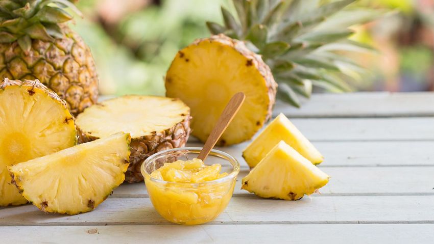
Fruit Flower
Pear Pineapple Strawberry Carnation Orchid Sunflower
Jackfruit Granny smith Acorn Rose Lotus Tulip
Unlabeled set 1 Labeled set 1 Labeled set 1.5 Labeled set 2 Unlabeled set 2
High similarity Medium similarity Low similarity
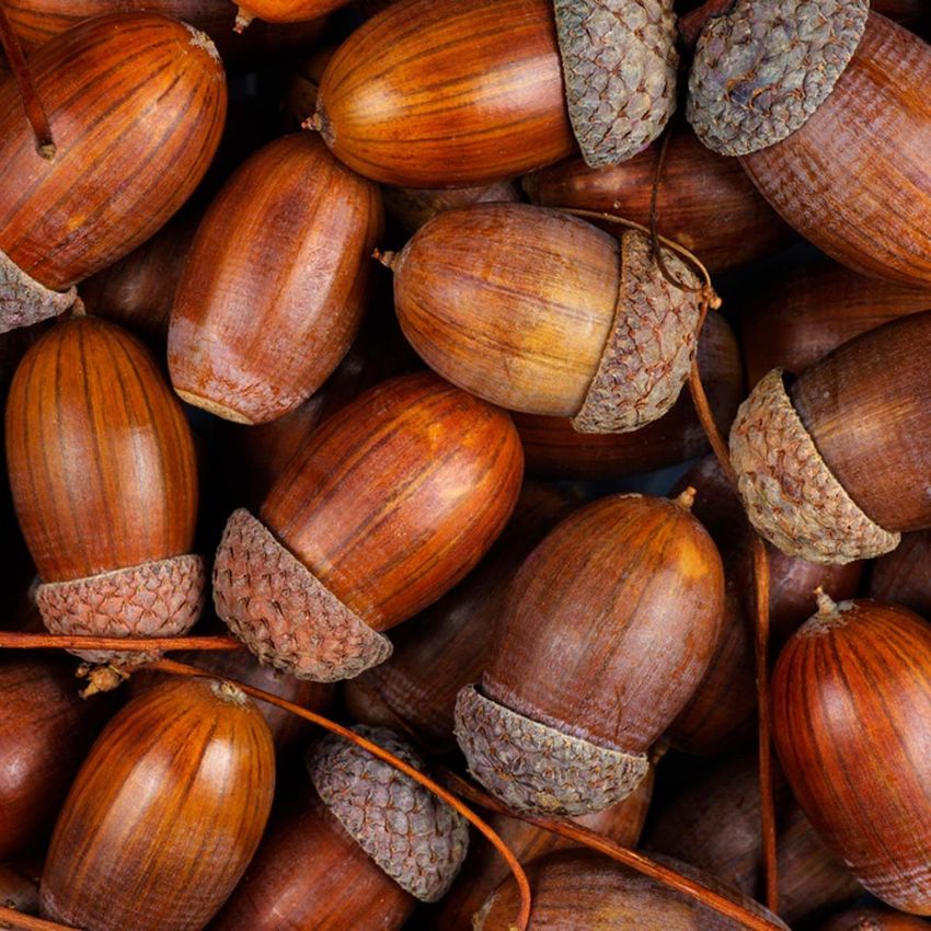
Figure 1: Illustration of how we construct the benchmark with varying levels of semantic similarity.
Unlabeled set U1 and labeled set L1 are from the same superclass (fruit), whereas unlabeled set U2
and labeled set L2 belong to another superclass (flower). Labeled set L1.5 is composed of half of L1
and half of L2 . If both the labeled and unlabeled classes are derived from the same superclass, i.e.
(U1 , L1 ) and (U2 , L2 ), we consider them a high semantic similarity split. In contrast, (U1 , L2 ) and
(U2 , L1 ) are low semantic similarity splits, since the labeled and unlabeled classes are derived from
distinct superclasses. In addition, we consider (U1 , L1.5 ) and (U2 , L1.5 ) to have medium semantic
similarity because half of L1.5 share the same superclass as U1 .
Table 1: Comparison of different semantic similarity settings in our proposed benchmark. L1 is
closely related to U1 and L2 is highly related to U2 . The third labeled set L1.5 is constructed from
half of L1 and half of L2 , so in terms of similarity it is in between L1 and L2 . For all splits we report
the mean and the standard deviation of the clustering accuracy across multiple NCD baselines.
Methods Unlabeled set U1 Unlabeled set U2
L1 - high L1.5 - medium L2 - low L1 - low L1.5 - medium L2 - high
K-means [16] 41.1 ± 0.4 30.2 ± 0.4 23.3 ± 0.2 21.2 ± 0.2 29.8 ± 0.4 45.0 ± 0.4
DTC [10] 43.3 ± 1.2 35.6 ± 1.3 32.2 ± 0.8 21.3 ± 1.2 15.3 ± 1.5 29.0 ± 0.8
RS [8] 55.3 ± 0.4 50.3 ± 0.9 53.6 ± 0.6 48.1 ± 0.4 50.9 ± 0.6 55.8 ± 0.7
NCL [22] 75.1 ± 0.8 74.3 ± 0.4 71.6 ± 0.4 61.3 ± 0.1 70.5 ± 0.8 75.1 ± 1.2
UNO [5] 83.9 ± 0.5 81.0 ± 0.5 77.2 ± 0.8 77.5 ± 0.7 82.0 ± 1.7 88.4 ± 1.2
Given a labeled set Ln = (Xl,i , Yl,i )ni=1 independently drawn from the labeled probability measure
PX,Y , and an unlabeled dataset Um = (Xu,i )m i=1 independently drawn from the unlabeled probability
measure QXu , our primary goal is to predict Yu,i given Xu,i , where Yu,i is the label of the i-th
unlabeled sample Xu,i .
Definition 1 (Novel class discovery) Let PXl ,Yl be a labeled probability measure on Xl × Cl , and
QXu ,Yu be an unlabeled probability measure on Xu × Cu , with Cu ∩ Cl = ∅. Given a labeled dataset
Ln sampled from PXl ,Yl and an unlabeled dataset Um sampled from QXu , novel class discovery
aims to predict the labels of the unlabeled dataset based on Ln and Um .
3.2 Transfer Leakage
We begin with introducing Maximum Mean Discrepancy (MMD) [7], which is used to measure the
discrepancy of two distributions. For example, the discrepancy of tworandom variables Z ∼ PZ
and Z0 ∼ PZ0 is defined as: MMDH PZ , PZ0 := supkhkH ≤1 E h(Z) − E h(Z0 ) where H is
a class of functions h : Xu → R, which is specified as a reproducing kernel Hilbert Space (RKHS)
associated with a continuous kernel function K(·, ·).
In NCD, the unlabeled dataset utilizes the conditional probability PYl |Xl (usually presented by a
pretrained neural network) from a labeled dataset. For example, if the distributions of PYl |Xl =Xu
under Yu = c and Yu = c0 are significantly different, then its overall distribution discrepancy is large,
3
yielding that more information can be leveraged in NCD. On this ground, we use MMD to quantify
the discrepancy of the labeled probability measure PYl |Xl on Xu under the unlabeled probability
measure Q, namely transfer leakage.

Definition 2 (Transfer leakage) The transfer leakage of NCD prediction under Q based on the
labeled conditional probability PYl |Xl is


                       T-Leak(Q, P) = EQ MMD2H Qp(Xu )|Yu , Qp(X0u )|Yu0 ,                               (1)

where (Xu , Yu ), (X0u , Yu0 ) ∼ Q are independent copies, the expectation EQ is taken with respect
to Yu and Yu0 under Q, and p(x) is the conditional probability under PYl |Xl on an unlabeled data
                                                          |
Xu = x, which is defined as p(x) = P Yl = c | Xl = x c∈C .
                                                                         l

To summarize, transfer leakage measures the overall discrepancy of p(Xu ) under different new
classes of the unlabeled measure Q, which indicates the informative leakage from P to Q. Next,
we give a finite sample estimate of transfer leakage. Given an estimated probability P   bY |X and an
                                                                                           l  l
                                 m
evaluation dataset (xu,i , yu,i )i=1 under Q, we assess xu,i on PYl |Xl as p
                                                                b          b (xu,i ) = P Yl = c|Xl =
                                                                                       b
    |
xu,i c∈Cu , then empirical transfer leakage is computed as:

                                 X            |Iu,c ||Iu,c0 | \ 2
          \
          T-Leak(Q, P) =                                      MMDH Qpb(Xu )|Yu =c , Qpb(X0u )|Yu0 =c ,   (2)
                                               m(m − 1)
                            c,c0 ∈Cu ;c6=c0

where the equality follows from the fact that MMD2H Qp(Xu )|Yu =c , Qp(X0u )|Yu0 =c = 0. Iu,c =

                                                                                                2
{1 ≤ i ≤ m : yu,i = c} is the index set of unlabeled data with yu,i = c, and M     \ MDH is defined in
                                      \
the Appendix. We use the proposed T-Leak to quantify the difficulty of NCD in various combination
of labeled and unlabeled sets. It is worth noting that the proposed transfer leakage and its empirical
evaluation depend only on the labeled/unlabeled datasets, and it remains the same, no matter what
NCD method we use. In addition, we provide pseudo transfer leakage (Appendix B.2), a practical
evaluation of the similarity between the classified and unlabeled sets. transfer leakage utilizes the true
label Yu , but the pseudo transfer leakage utilizes the pseudo label obtained from clustering methods
(e.g., k-means) on the representations. Further information is available in Appendix B.

4     Supervised Knowledge may be Harmful

The motivation behind NCD is that supervised knowledge from labeled data can enhance unlabeled
data clustering. Counterintuitively, we observe that supervised information from a labeled set
may result in suboptimal outcomes compared to exclusively self-supervised knowledge. Further
information is provided in Appendix C.2.

4.1   Experiments and Results

To investigate, we conduct experiments in the following settings: (1) Using the unlabeled set, Xu ;
(2) Using the unlabeled set and the labeled set’s images without labels, Xu + Xl ; (Even without
labels, self-supervised learning can extract the knowledge from labeled set’s image.) (3) Using the
unlabeled set and the whole labeled set, Xu + (Xl , Yl ), (i.e., standard NCD). As suggested in Table
2, NCD performance is consistently improved by incorporating more images (without labels) from a
labeled set, around 10% on CIFAR100 and 6%-18% in our benchmark. By comparing (2) and (3),
we can isolate the impact of the labels. Unexpectedly, on CIFAR100-50 and ImageNet with low
semantic similarity, (3) performs around 2 - 8% worse than (2), yielding that “low-quality" supervised
information may hurt NCD performance.

                                                         4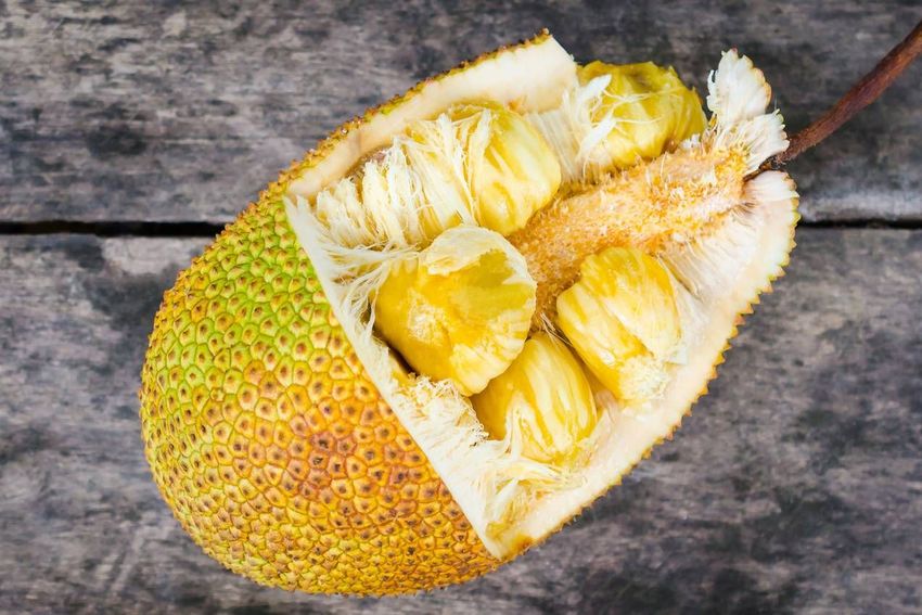
Table 2: Comparison of different data settings on CIFAR100 and our proposed benchmark. We
present clustering mean and standard error on SOTA method, UNO. (1) uses only the unlabeled set,
whereas (2) uses both the unlabeled set and the labeled set’s images without labels. (3) represents the
standard NCD setting, i.e., using the unlabeled set and the whole labeled set. Counterintuitively, in
CIFAR100-50 and low similarity case of our benchmark, (2) can get greater performance than (3).
                                                      Unlabeled set U1              Unlabeled set U2
      Setting                  CIFAR100-50
                                                   L1 - high       L2 - low        L1 - low      L2 - high
      (1) Xu                    54.9 ± 0.4         70.5 ± 1.2      70.5 ± 1.2   71.9 ± 0.3     71.9 ± 0.3
      (2) Xu + Xl               64.1 ± 0.4         79.6 ± 1.1      80.3 ± 0.3   85.3 ± 0.5     89.2 ± 0.3
      (3) Xu + (Xl , Yl )       62.2 ± 0.2         83.9 ± 0.6      77.2 ± 0.8   77.5 ± 0.7     88.3 ± 1.1

4.2    Practical Applications

As shown above, supervised knowledge from the labeled set may cause damage, but it’s difficult
to determine whether to utilize it or self-supervised knowledge. Therefore, we offer two concrete
solutions, a practical metric (i.e., pseudo transfer leakage) and a straightforward method.

Supervised or Self-supervised Knowledge? The proposed pseudo transfer leakage is a practical
reference to infer what kind of data we want to employ in NCD, images-only information or image-
label pairs. In Table 3 (PTL), we compute pseudo transfer leakage via a supervised model and a
self-supervised model based on pseudo labels. As suggested in Table 3 (ACC), the pseudo transfer
leakage is consistent with the accuracy based on various datasets. For example, in L1 -U1 , the pseudo
transfer leakage computed on the supervised model is larger than the one computed in the self-
supervised model, which is consistent with the accuracy, where the supervised method outperforms
the self-supervised one.

Combining Supervised and Self-supervised Knowledge Instead of using either supervised
knowledge or self-supervised knowledge from the labeled set, we propose an effective and straight-
forward method, which smoothly combines both of them. We combine the labeled set’s ground truth
labels ylGT with self-supervised pseudo labels ylP L . αylGT + (1 − α)ylP L is the overall classification
objective, where α ∈ [0, 1] is the supervised component weight. This strategy has the same aim
as UNO [5] for α = 1, but uses self-supervised pretraining instead of supervised. As shown in
Figure 3, our proposed method improves CIFAR100 and ImageNet by 3% and 5%, respectively,
compared to UNO. Our method delivers significant improvements for low semantic similarity cases
and competitive performances for high similarity cases.

Table 3: Results showing the link between pseudo transfer leakage (PTL) and accuracy on novel
classes (ACC). The pseudo transfer leakage is computed based either on a supervised (SL) or self-
supervised model (SSL), using ResNet18 in both cases. The accuracy is obtained using the standard
NCD setting (Xu + (Xl , Yl )) for supervised learning, and self-supervised NCD (Xu + Xl ) for the
self-supervised model.

                            High similarity              Medium similarity                Low similarity
         Model
                    L1 − U1           L2 − U2         L1.5 − U1       L1.5 − U2        L2 − U1        L1 − U2

PTL       SSL      0.96 ± 0.01       0.96 ± 0.02     1.14 ± 0.02      1.19 ± 0.01    1.05 ± 0.03    1.25 ± 0.03
          SL       1.21 ± 0.02       1.21 ± 0.01     1.03 ± 0.02      0.98 ± 0.03    0.99 ± 0.02    0.96 ± 0.01
          SSL      79.6 ± 1.1        89.2 ± 0.3       79.7 ± 1.0      85.2 ± 1.0      80.3 ± 0.3     85.3 ± 0.5
ACC
          SL       83.9 ± 0.6        88.3 ± 0.5       81.0 ± 0.6      82.0 ± 1.6      77.2 ± 0.8     77.5 ± 0.7

5     Conclusion
We first offer a comprehensive ImageNet-based benchmark with varying levels of semantic similarity
and show that semantic similarity affects NCD performance. Second, we present transfer leakage, a
semantic similarity metric. Furthermore, we find that in low semantic similarity situations, labeled
information may lead to inferior performance. We propose two practical applications based on these
findings: (i) Using transfer leakage to determine what data to use. (ii) a straightforward approach
that improves CIFAR100 and ImageNet by 3-5%.

                                                        5
References
 [1] Caron, M., Misra, I., Mairal, J., Goyal, P., Bojanowski, P., Joulin, A.: Unsupervised learning of visual
     features by contrasting cluster assignments. Advances in Neural Information Processing Systems 33,
     9912–9924 (2020)
 [2] Chi, H., Liu, F., Yang, W., Lan, L., Liu, T., Han, B., Niu, G., Zhou, M., Sugiyama, M.: Meta discovery:
     Learning to discover novel classes given very limited data. In: ICLR (2021)
 [3] Cuturi, M.: Sinkhorn distances: lightspeed computation of optimal transport. In: Proceedings of the 26th
     International Conference on Neural Information Processing Systems-Volume 2, pp. 2292–2300 (2013)
 [4] Deng, J., Dong, W., Socher, R., Li, L.J., Li, K., Fei-Fei, L.: Imagenet: A large-scale hierarchical image
     database. In: CVPR, pp. 248–255, IEEE (2009)
 [5] Fini, E., Sangineto, E., Lathuilière, S., Zhong, Z., Nabi, M., Ricci, E.: A unified objective for novel class
     discovery. In: ICCV, pp. 9284–9292 (2021)
 [6] Garg, S., Balakrishnan, S., Lipton, Z.C.: Domain adaptation under open set label shift. arXiv preprint
     arXiv:2207.13048 (2022)
 [7] Gretton, A., Borgwardt, K.M., Rasch, M.J., Schölkopf, B., Smola, A.: A kernel two-sample test. The
     Journal of Machine Learning Research 13(1), 723–773 (2012)
 [8] Han, K., Rebuffi, S.A., Ehrhardt, S., Vedaldi, A., Zisserman, A.: Automatically discovering and learning
     new visual categories with ranking statistics. In: International Conference on Learning Representations
     (2020)
 [9] Han, K., Rebuffi, S.A., Ehrhardt, S., Vedaldi, A., Zisserman, A.: Autonovel: Automatically discovering
     and learning novel visual categories. IEEE Transactions on Pattern Analysis and Machine Intelligence
     (2021)
[10] Han, K., Vedaldi, A., Zisserman, A.: Learning to discover novel visual categories via deep transfer
     clustering. In: CVPR (2019)
[11] He, K., Zhang, X., Ren, S., Sun, J.: Deep residual learning for image recognition. In: Proceedings of the
     IEEE conference on computer vision and pattern recognition, pp. 770–778 (2016)
[12] Hsu, Y.C., Lv, Z., Kira, Z.: Learning to cluster in order to transfer across domains and tasks. arXiv preprint
     arXiv:1711.10125 (2017)
[13] Hsu, Y.C., Lv, Z., Kira, Z.: Learning to cluster in order to transfer across domains and tasks. In: International
     Conference on Learning Representations (2018)
[14] Hsu, Y.C., Lv, Z., Schlosser, J., Odom, P., Kira, Z.: Multi-class classification without multi-class labels. In:
     International Conference on Learning Representations (2019)
[15] Krizhevsky, A.: Learning multiple layers of features from tiny images (2009)
[16] MacQueen, J., et al.: Some methods for classification and analysis of multivariate observations. In:
     Proceedings of the fifth Berkeley symposium on mathematical statistics and probability, vol. 1, pp. 281–
     297, Oakland, CA, USA (1967)
[17] Miller, G.A.: Wordnet: a lexical database for english. Communications of the ACM 38(11), 39–41 (1995)
[18] Santurkar, S., Tsipras, D., Madry, A.: Breeds: Benchmarks for subpopulation shift. In: ICLR (2020)
[19] Vinyals, O., Blundell, C., Lillicrap, T., Wierstra, D., et al.: Matching networks for one shot learning.
     Advances in neural information processing systems 29 (2016)
[20] Xie, J., Girshick, R., Farhadi, A.: Unsupervised deep embedding for clustering analysis. In: International
     conference on machine learning, pp. 478–487, PMLR (2016)
[21] Zhao, B., Han, K.: Novel visual category discovery with dual ranking statistics and mutual knowledge
     distillation. NIPS (2021)
[22] Zhong, Z., Fini, E., Roy, S., Luo, Z., Ricci, E., Sebe, N.: Neighborhood contrastive learning for novel class
     discovery. In: CVPR (2021)
[23] Zhong, Z., Zhu, L., Luo, Z., Li, S., Yang, Y., Sebe, N.: Openmix: Reviving known knowledge for
     discovering novel visual categories in an open world. In: CVPR (2021)

                                                          6
A     Details of Section 2

A.1   Assumption

Existing benchmarks consider the difficulty of NCD in terms of the labeled set from two aspects: (1)
the number of categories, e.g. [5] propose a more challenging benchmark called CIFAR100-50 (i.e.,
50/50 classes for unlabeled/labeled set), compared to the commonly used CIFAR100-20 (i.e., 20/80
classes for unlabeled/labeled set). (2) The number of images in each category, [2] propose to use less
images for each labeled’s class.
However, in addition to the number of categories and images, another significant factor is the
semantic similarity between the two sets. As mentioned in [2], NCD is theoretically solvable when
labeled and unlabeled sets share high-level semantic features. Based on this, we conduct a further
investigation with the assumption that more similar labeled sets (when the number of categories
and images are fixed) can lead to better performance. Intuitively, according to Figure 1, despite
the fact that the labeled (e.g., pineapple, strawberry) and unlabeled (e.g., pear, jackfruit) classes are
disjoint, if they derive from the same superclass (i.e., fruit), they have a higher degree of semantic
similarity. Conversely, when labeled (e.g., rose, lotus) and unlabeled (e.g., pear, jackfruit) classes
are derived from distinct superclasses (i.e., labeled classes from flower while unlabeled classes from
fruit), they are further apart semantically. Consequently, we construct various semantic similarity
labeled/unlabeled settings based on a hierarchical class structure and evaluate our assumption on
CIFAR100 and ImageNet.

A.2   Benchmark

Existing benchmarks in the field were created without regard to the semantic similarity between
labeled and unlabeled set. Most works follow the standard splits introduced in [10]. In CIFAR10 [15],
the labeled set is made up of the first five classes in alphabetical order, and the unlabeled set of the
remaining five. A similar approach was taken with the commonly used CIFAR100-20 and CIFAR100-
50 benchmarks. A benchmark based on ImageNet [4] has one labeled set, with 882 classes and three
unlabeled sets. Each of these unlabeled sets contains 30 classes, which were randomly selected from
the remaining non-labeled classes [19, 12, 14, 10].
To address this limitation and allow for an evaluation of our assumptions, we propose a new benchmark
based on ImageNet including three different semantic similarity levels (high, medium and low). As
mentioned in Section A.1, we separate labeled and unlabeled classes by leveraging ImageNet’s
underlying hierarchy. While ImageNet is based on the WordNet hierarchy [17], it is not well-suited
for this purpose as discussed by [18]. To address these issues, they propose a modified hierarchy and
define multiple hierarchical classification tasks based on it. While originally defined to measure the
impact of subpopulation shift, they can also be used to define NCD tasks.
Our proposed benchmark is based on the ENTITY-30 task, which contains 240 ImageNet classes in
total, with 30 superclasses and 8 subclasses for each superclasses. For example, as shown in Figure 1,
we define three labeled sets L1 , L2 and L1.5 and two unlabeled sets U1 and U2 . The sets L1 and
U1 are selected from the first 15 superclasses, with 6 subclasses of each superclass assigned to L1
and the other 2 assigned to U1 . The sets L2 and U2 are created from the second 15 superclasses in
a similar fashion. Finally, L1.5 is created by taking half the classes from L1 and half of the classes
from L2 . Therefore, (U1 , L1 )/(U2 , L2 ) are highly related semantically, (U1 , L2 )/(U2 , L1 ) belong
to the low semantic cases and (U1 , L1.5 )/(U2 , L1.5 ) are the medium cases. Additionally, we also
create four data settings on CIFAR100, with two high semantic cases and two low semantic cases by
leveraging CIFAR100 hierarchical class structure. Each case has 40 labeled classes and 10 unlabeled
classes. A full list of the labeled and unlabeled sets with their respective superclasses and subclasses
can be found in Appendix G.
This benchmark setup allows us to systematically investigate the influence of the labeled set on a
large benchmark dataset. By keeping the unlabeled set constant and varying the used labeled set, we
can isolate the influence of semantic similarity on NCD performance.

                                                   7
A.3   Experimental Setup and Results

To verify our assumption, we conduct experiments on four competitive baselines, including K-means
[16], DTC [10], RS [9], NCL [22] and UNO [5]. We follow the baselines regarding hyperparameters
and implementation details.

Results on CIFAR100 In Table 4, U1 and U2 represent the unlabeled sets, while L1 and L2
represent the labeled sets. U1 /U2 and L1 /L2 share the same super classes, while U1 /U2 and L2 /L1
belong to different super classes. We evaluate 4 different labeled/unlabeled settings in CIFAR100,
with 2 high semantic cases (i.e., (U1 , L1 ) and (U2 , L2 )) and low semantic cases (i.e., (U1 , L2 ) and
(U2 , L1 )). The gap between the high-similarity and the low-similarity settings is larger than 20% for
K-means, and reaches up to 12% for more advanced methods. The strong results of UNO across all
splits show that a more difficult benchmark is needed to obtain clear results for future methods.

Results on our proposed benchmark Similarly, in Table 1, the most similar labeled set generally
obtains the best performance, followed by the medium and the least similar one. Under the unlabeled
set U1 , L1 achieves the highest accuracy, with around 2-17% improvement compared to L2 , and
around 2-11% improvement compared to L1.5 . For the unlabeled set U2 , L2 is the most similar set
and obtains 8-14% improvement compared to L1 , and around 5-14% improvement compared to L1.5 .
Table 4: Comparison of different combinations of labeled sets and unlabeled sets consisting of
subsets of CIFAR100. The unlabeled set are denoted U1 and U2 , while the labeled sets are called L1
and L2 . U1 and L1 share the same set of superclasses, similar for U2 and L2 . Thus, the pairs (U1 ,
L1 ) and (U2 , L2 ) are close semantically, but (U1 , L2 ) and (U2 , L1 ) are far apart. For all splits we
report the mean and standard deviation of the clustering accuracy across multiple NCD methods.

                                        Unlabeled set U1               Unlabeled set U2
            Methods
                                   L1 - high       L2 - low      L1 - low         L2 - high
            K-means [16]          61.0 ± 1.1      37.7 ± 0.6    33.9 ± 0.5        55.4 ± 0.6
            DTC [10]              64.9 ± 0.3      62.1 ± 0.3    53.6 ± 0.3        66.5 ± 0.4
            RS [8]                78.3 ± 0.5      73.7 ± 1.4    74.9 ± 0.5        77.9 ± 2.8
            NCL [22]              85.0 ± 0.6      83.0 ± 0.3    72.5 ± 1.6        85.6 ± 0.3
            UNO [5]               92.5 ± 0.2      91.3 ± 0.8    90.5 ± 0.7        91.7 ± 2.2

B     Details of Section 3

B.1   The Detailed Derivation Process of Transfer Leakage

To summarize, transfer leakage measures the overall discrepancy of p(Xu ) under different new
classes of the unlabeled measure Q, which indicates the informative leakage from P to Q.

Definition 3 (Transfer leakage) The transfer leakage of NCD prediction under Q based on the
labeled conditional probability PYl |Xl is

                     T-Leak(Q, P) = EQ MMD2H Qp(Xu )|Yu , Qp(X0u )|Yu0 ,                (3)

where (Xu , Yu ), (X0u , Yu0 ) ∼ Q are independent copies, the expectation EQ is taken with respect
to Yu and Yu0 under Q, and p(x) is the conditional probability under PYl |Xl on an unlabeled data
                                                          |
Xu = x, which is defined as p(x) = P Yl = c | Xl = x c∈C .
                                                                   l

Next, we give a finite sample estimate of transfer leakage. To proceed, we first rewrite transfer
leakage as follows.
                         X
                                Q(Yu = c, Yu0 = c0 )MMD2H Qp(Xu )|Yu =c , Qp(X0u )|Yu0 =c0 ,

    T-Leak(Q, P) =                                                                            (4)
                      c,c0 ∈Cu ;c6=c0

where the equality follows from the fact that MMD2H Qp(Xu )|Yu =c , Qp(X0u )|Yu0 =c = 0.


                                                     8
bY |X and an evaluation dataset (xu,i , yu,i )m under Q, we assess
Given an estimated probability P l  l                                        i=1
                              b Yl = c|Xl = xu,i | , then the empirical transfer leakage is

xu,i on P
        bY |X as p
          l  l
                 b (xu,i ) = P                       c∈Cu
computed as:
                                 X            |Iu,c ||Iu,c0 | \ 2
          \
          T-Leak(Q, P) =                                      MMDH Qpb(Xu )|Yu =c , Qpb(X0u )|Yu0 =c ,               (5)
                                               m(m − 1)
                            c,c0 ∈Cu ;c6=c0

                                                                                                                         2
where Iu,c = {1 ≤ i ≤ m : yu,i = c} is the index set of unlabeled data with yu,i = c, and M \  MDH
is defined as:
          2                                                1          X
   M\ MDH (Qpb(Xu )|Yu =c , Qpb(X0u )|Yu0 =c ) =                        K pb (xu,i ), p
                                                                                      b (xu,j )
                                                 |Iu,c |(|Iu,c | − 1)
                                                                            i,j∈Iu,c ;i6=j
                                                               1                  X
                                                +                                              K p
                                                                                                 b (xu,i ), p
                                                                                                            b (xu,j )
                                                    |Iu,c0 |(|Iu,c0 | − 1)
                                                                             i,j∈Iu,c0 ;i6=j

                                                           2           X      X
                                                −                                      K p
                                                                                         b (xu,i ), p
                                                                                                    b (xu,j ) .
                                                    |Iu,c ||Iu,c0 |
                                                                      i∈Iu,c j∈Iu,c0

B.2   Pseudo Transfer Leakage

In practice, the ground-truth labels of the unlabeled set are difficult to acquire. Therefore, we utilize
pseudo labels derived from clustering algorithms, e.g., k-means, rather than true labels in computing
transfer leakage, and we named it as pseudo transfer leakage

Definition 4 (Pseudo Transfer Leakage)
                                  X            |Ieu,c ||Ieu,c0 | \2
           \
          PT-Leak(Q, P) =                                        MMDH Qpb(Xu )|Yeu =c , Qpb(X0 )|Ye 0 =c             (6)
                                                m(m − 1)                                     u     u
                             c,c0 ∈Cu ;c6=c0

where Ieu,c = {1 ≤ i ≤ m : yeu,i = c} is the index set of unlabeled data with yeu,i = c, yeu,i
                                                      s(xu,i ), and b
is provided based on k-means on their representations b             s(xu,i ) is the representation
                                                                     2
estimated from a supervised model or a self-supervised model. MMDH is defined similarly as in
                                                                \
Section 3.

Pseudo transfer leakage, a practical evaluation of the similarity between the classified and unlabeled
sets, could be a practical reference on whether to images-only or image-label pairs information from
the labeled set.

B.3   The Lower and Upper Bounds of Transfer Leakage

Lemma 1 shows the lower and upper bounds of transfer leakage, and provide a theoretical justification
that it is a effective quantity to measure the similarity between labeled and unlabeled datasets.
                                      p
Lemma 1 Let κ := maxc∈Cu EQ             K(p(Xu ), p(Xu ))|Yu = c < ∞, then 0 ≤ T-Leak(Q, P) ≤
4κ2 . Moreover, T-Leak(Q, P) = 0 if and only if Yu is independent with p(Xu ), that is, for any
c ∈ Cu :
                                   Q Yu = c | p(Xu ) = Q(Yu = c),                                 (7)
yielding that p(Xu ) is useless in NCD on Q.

Note that κ can be explicitly computed for many common used kernels, for example, κ = 1 for a
Gaussian or Laplacian kernel. From Lemma 1, T-Leak(Q, P) = 0 is equivalent to Yu is independent
with p(Xu ), which matches our intuition of no leakage. Alternatively, if Yu is dependent with p(Xu ),
we justifiably believe that the information of Yl |Xl can be used to facilitate NCD, Lemma 1 tells that
T-Leak(Q, P) > 0 in this case. Therefore, Lemma 1 reasonably suggests that the proposed transfer
leakage is an effective metric to detect if the labeling information in P is useful to NCD on Q.

                                                          9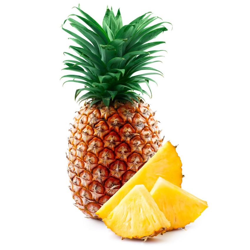
Proof of Lemma 1. We first show the upper bound of the transfer leakage. According to Lemma 3
in [7], we have

                                                                                     2
T-Leak(Q, P) = EQ MMD2 (Qs(Xu )|Yu , Qs(X0u )|Yu0 ) = EQ µQs(Xu )|Yu − µQs(X0 )|Y 0 H

                                                                                       u    u
                                                           2
                 ≤ max
                    0
                          µQs(Xu )|Yu =c − µQs(X0 )|Y 0 =c0H
                                                              ≤ 4 max kµQs(Xu )|Yu =c k2H
                   c,c ∈Cu                      u     u           c∈Cu

                 = 4 maxhEQ K(s(Xu ), ·)|Yu = c , EQ K(s(X0u ), ·)|Yu0 = c iH

                     c∈Cu

                 = 4 max EQ hK(s(Xu ), ·), K(s(X0u ), ·)iH |Yu = c, Yu0 = c

                     c∈Cu

                 ≤ 4 max EQ K(s(Xu ), ·) H K(s(X0u ), ·) H |Yu = c, Yu0 = c
                     c∈Cu
                             p                                  p
                                                                  K(s(X0u ), s(X0u ))|Yu0 = c ≤ 4κ2 ,

                 = 4 max EQ    K(s(Xu ), s(Xu ))|Yu = c EQ
                     c∈Cu

where µQs(Xu )|Yu := EQ K(s(Xu ), ·)|Yu is the kernel mean embedding of the measure Qs(Xu )|Yu
[7], the second inequality follows from the triangle inequality in the Hilbert space, the fourth equality
follows from the fact that EQ is a linear operator, the second last inequality follows from the Cauchy-
Schwarz inequality, and the last equality follows the reproducing property of K(·, ·).
Next, we show the if and only if condition for T-Leak(Q, P) = 0. Assume that Q(Yu = c) > 0 for
all c ∈ Cu . According to Theorem 5 in [7], we have

            T-Leak(Q, P) = 0    ⇐⇒       Q s(x)|Yu = c = q0 (x), for c ∈ Cu , x ∈ Xu .

Note that
      X                         X Q(s(x)|Yu = c)Q(Yu = c)   X q0 (x)Q(Yu = c)    q0 (x)
1=           Q(Yu = c|s(x)) =                             =                   =         ,
                                          Q(s(x))                  Q(s(x))      Q(s(x))
      c∈Cu                      c∈Cu                                 c∈Cu

yielding that Q s(x)|Yu = c = Q(s(x)), for c ∈ Cu , x ∈ Xu . This is equivalent to,

                                Q s(x)|Yu = c Q(Yu = c)
                  Q Yu = c|s(x) =                               = Q(Yu = c).
                                             Q(s(x))

This completes the proof.

B.4    Experiments and Results

Experimental Setup and Hyperparameters To calculate the transfer leakage/pseudo transfer
leakage, we employ ResNet18 [11] as the backbone for both datasets following [10, 9, 5]. Known-
class data and unknown-class data are selected based on semantic similarity, as mentioned in Section
2. We first apply fully supervised learning to the labeled data for each data set to obtain the pretrained
model. Then, we feed the unlabeled data to the pretrained model to obtain its representation. Lastly,
we calculate the transfer leakage/pseudo transfer leakage based on the pretrained model and the
unlabeled samples’ representation. Speciallly, for pseudo transfer leakage, we apply clustering
methods to generate the pseudo labels. For the first step, batch size is set to 512 for both datasets. We
use an SGD optimizer with momentum 0.9, and weight decay 1e-4. The learning rate is governed
by a cosine annealing learning rate schedule with a base learning rate of 0.1, a linear warmup of 10
epochs, and a minimum learning rate of 0.001. We pretrain the backbone for 200/100 epochs for
CIFAR-100/ImageNet.

Results Figure 2 shows semantic similarity, transfer leakage/pseudo transfer leakage and NCD per-
formance on ImageNet, in which the same color corresponds to the same unlabeled set. As expected,
splits that have a higher semantic similarity yield both higher transfer leakage and pseudo transfer
leakage. Alternatively, there is a consistent positive correlation between transfer leakage/pseudo
transfer leakage and NCD accuracy, which confirms the validity of transfer leakage/pseudo transfer
leakage as a metric in quantifying semantic similarity and the difficulty of a particular NCD problem.

                                                   10
Low similarity Medium similarity High similarity
UNO NCL K-means U1 U2
90 90
Accuracy in % 80 80
Accuracy in %
70 70
60 60
50 50
40 40
30 30
0.3 0.5 0.7 0.9 1.1 1.3
Transfer-leakage Pseudo Transfer-leakage
Figure 2: Experiments on transfer leakage and pseudo transfer leakage. Each line stands for one
unlabeled set from our proposed ImageNet-based benchmark, and each point on the line for one
labeled / unlabeled split. On the left, we measure the transfer leakage and the clustering accuracy
obtained using UNO, NCL and k-means for each split. As expected, there is a positive correlation
between semantic similarity and transfer leakage as well as between transfer leakage and accuracy.
On the right, we replace transfer leakage with pseudo transfer leakage obtained using k-means
clustering. The comparison shows that pseudo transfer leakage can in practice be used as a proxy for
transfer leakage.
Table 5: Experiments on the stability of pseudo transfer leakage and transfer leakage. To obtain the
standard deviation we recompute the transfer leakage and pseudo transfer leakage 10 times using
bootstrap sampling. The results show that both transfer leakage has a low random variation.
Dataset Unlabeled Set Labeled Set Transfer leakage Pseudo transfer leakage
L1 0.62 ± 0.01 0.89 ± 0.06
U1
L2 0.28 ± 0.01 0.74 ± 0.04
CIFAR100
L1 0.33 ± 0.01 0.73 ± 0.02
U2
L2 0.77 ± 0.02 1.24 ± 0.01
L1 0.71 ± 0.01 1.21 ± 0.02
U1 L1.5 0.54 ± 0.01 1.03 ± 0.02
L2 0.36 ± 0.01 0.99 ± 0.02
ImageNet
L1 0.33 ± 0.00 0.96± 0.01
U2 L1.5 0.50 ± 0.01 0.98± 0.03
L2 0.72 ± 0.01 1.21± 0.01
Table 6: Experiments on pseudo transfer leakage under three clustering methods, i.e., k-means,
GMM and agglomerative, and each setting is repeated for 10 times.
Unlabeled set U1 Unlabeled set U2
Method
L1 - high L1.5 - medium L2 - low L1 - low L1.5 - medium L2 - high
k-means 1.23 ± 0.03 1.02 ± 0.03 0.99 ± 0.02 0.96 ± 0.01 0.99 ± 0.03 1.24 ± 0.02
GMM 0.79 ± 0.01 0.69 ± 0.02 0.56 ± 0.02 0.58 ± 0.02 0.68 ± 0.04 0.91 ± 0.02
Agglomerative 1.17 ± 0.00 0.96 ± 0.00 0.87 ± 0.00 0.83 ± 0.00 0.89 ± 0.00 1.15 ± 0.00
11C Details of Section 4
C.1 Counterintuitive Observations
The motivation behind NCD is that prior supervised knowledge from labeled data can help improve
the clustering of the unlabeled set. However, we have counterintuitive results: supervised information
from a labeled set may result in suboptimal outcomes as compared to using exclusively self-supervised
knowledge. To investigate, we conduct experiments in the following settings:
(1) Using the unlabeled set, Xu
(2) Using the unlabeled set and the labeled set’s images without labels, Xu + Xl
(3) Using the unlabeled set and the whole labeled set, Xu + (Xl , Yl ), (i.e., standard NCD).
Specifically, for (1), NCD is degenerated to unsupervised learning (i.e., clustering on Xu ). For (2),
even though we do not use the labels, we can still try to extract the knowledge of the labeled set
via self-supervised learning. By comparing (1) and (3), we can estimate the total performance gain
caused by adding the labeled set. The comparison between (1) and (2) as well as (2) and (3) allows
us to further disentangle the performance gain according to the components of the labeled set.
Table 7: Comparison of different data settings on CIFAR100 and the unlabeled set U1 of our proposed
benchmark. We report the mean and the standard error of the clustering accuracy of UNO. As UNO
uses multiple unlabeled heads, we report their mean accuracy, as well as that of the head with the
lowest loss. Setting (1) uses only the unlabeled set, whereas (2) uses both the unlabeled set and the
labeled set’s images without labels. Setting (3) represents the standard NCD setting, i.e., using the
unlabeled set and the whole labeled set. Counterintuitively, in CIFAR100-50 and on the low similarity
case of our benchmark, we can achieve better performance without using the labeled set’s labels.
ImageNet U1
UNO Setting CIFAR100-50
L1 - high L1.5 - medium L2 - low
(1) Xu 54.2 ± 0.3 69.2 ± 0.7 69.2 ± 0.7 69.2 ± 0.7
Avg head (2) Xu + Xl 63.4 ± 0.4 74.9 ± 0.3 77.6 ± 0.9 77.9 ± 1.1
(3) Xu + (Xl , Yl ) 61.7 ± 0.3 81.7 ± 1.0 80.3 ± 0.4 74.6 ± 0.3
(1) Xu 54.9 ± 0.4 70.5 ± 1.2 70.5 ± 1.2 70.5 ± 1.2
Best head (2) Xu + Xl 64.1 ± 0.4 79.6 ± 1.1 79.7 ± 1.0 80.3 ± 0.3
(3) Xu + (Xl , Yl ) 62.2 ± 0.2 83.9 ± 0.6 81.0 ± 0.6 77.2 ± 0.8
Table 8: Comparison of different data settings on the unlabeled set U2 of our proposed benchmark,
similar to Table 7. We report the mean and the standard error of the clustering accuracy of UNO.
ImageNet U2
UNO Setting
L1 - low L1.5 - medium L2 - high
(1) Xu 68.4 ± 0.6 68.4 ± 0.6 68.4 ± 0.6
Avg head (2) Xu + Xl 81.0 ± 0.4 81.6 ± 1.1 85.9 ± 0.8
(3) Xu + (Xl , Yl ) 76.2 ± 0.6 80.0 ± 1.6 87.5 ± 1.2
(1) Xu 71.9 ± 0.3 71.9 ± 0.3 71.9 ± 0.3
Best head (2) Xu + Xl 85.3 ± 0.5 85.2 ± 1.0 89.2 ± 0.3
(3) Xu + (Xl , Yl ) 77.5 ± 0.7 82.0 ± 1.6 88.3 ± 1.1
Experimental Setup We conduct experiments on UNO [5], which is to the best of our knowledge
the current state-of-the-art method in NCD. To perform experiments (1) and (2), we make adjustments
on the framework of UNO, enabling it to run fully self-supervised. This is done by replacing the
labeled set’s ground truth labels ylGT with self-supervised pseudo labels ylP L , which are obtained by
applying the Sinkhorn-Knopp algorithm [3].
The standard UNO method conducts NCD in a two-step approach. In the first step, it applies a
supervised pretraining on the labeled data only. The pretrained model is then used as an initialization
12for the second step, in which the model is trained jointly on both labeled and unlabeled data using
one labeled head and multiple unlabeled heads.
To adapt UNO to the fully unsupervised setting in (1), we need to remove all parts that utilize the
labeled data. Therefore, in the first step, we replace the supervised pretraining by a self-supervised
one, which is trained only on the unlabeled data. For the second step, we simply remove the labeled
head, thus the method is degenerated to a clustering approach based solely on the pseudo-labels
generated by the Sinkhorn-Knopp algorithm. For setting (2), we apply the self-supervised pretraining
based on both unlabeled and labeled images to obtain the pretrained model in the first step. In the
second step, we replace the ground-truth labels for the known classes with pseudo-labels generated
by the Sinkhorn-Knopp algorithm based on the logits of these classes. Taken together, the updated
setup utilizes the labeled images, but not their labels.
Hyperparameters We conduct our experiments on CIFAR100 as well as our proposed ImageNet-
based benchmark. All settings and hyperparameters are kept as close as possible as to the original
baselines, including the choice of ResNet18 as the model architecture. We use SWAV [1] as self-
supervised pretraining for all experiments. The pretraining is done using the small batch size
configuration of the method, which uses a batch size of 256 and a queue size of 3840. The training is
run for 800 epochs, with the queue being enabled at 60 epochs for our ImageNet-based benchmark
and 100 epochs for CIFAR100. To ensure a fair comparison with the standard NCD setting, the same
data augmentations were used. In the second step of UNO, we train the methods for 500 epochs on
CIFAR100 and 100 epochs for each setting on our benchmark. The experiments are replicated 10
times on CIFAR100 and 5 times on the developed benchmark, and the averaged performances and
their corresponding standard errors are summarized in Table 7.
Results As suggested in Table 7 and Table 8, NCD performance is consistently improved by
incorporating more images (without labels) from a labeled set, the percentages of improvements in
terms of accuracy are around 10% on CIFAR100 (comparing (1) and (2)). For our benchmark, the
setting (2) obtains an improvement about 6 - 10% over (1) and the increase is more obvious in the
lower semantic similarity cases. Similarly, by comparing (2) and (3), we can isolate the impact of
the labels. For this case, the largest percentage of improvement, about 4 - 7%, is obtained in the
high-similarity setting, followed by the the medium-similarity setting with 1 - 3% improvements.
Interestingly, on CIFAR100-50 and ImageNet with low semantic similarity, we unexpectedly observe
that (2) performs around 2 - 8% better than (3), yielding that “low-quality" supervised information
may hurt NCD performance.
C.2 Practical Applications
As shown in Table 7 and Table 8, even though we find that supervised knowledge from the labeled set
may cause harm rather than gain, it is still difficult to decide whether to utilize supervised knowledge
with labeled data or just pure self-supervised knowledge without labels. Therefore, we offer two
concrete solutions, a practical metric (i.e., pseudo transfer leakage) and a straightforward method.
The proposed pseudo transfer leakage is a practical reference to infer what sort of data we want to use
in NCD, images-only information, Xu + Xl or the image-label pairs, Xu + (Xl , Yl ) from the labeled
set. In Table 3, we compute pseudo transfer leakage via a supervised model and a self-supervised
model based on pseudo labels. As suggested„ the pseudo transfer leakage is consistent with the
accuracy based on various datasets. For example, in L1 − U1 , the pseudo transfer leakage computed
on the supervised model is larger than the one computed in the self-supervised model, which is
consistent with accuracy, the supervised method outperforms the self-supervised one. Reversely, for
L2 -U1 , L1 -U2 and L1.5 − U1 , the pseudo transfer leakage computed on the self-supervised model is
larger than the one computed in the supervised model, which is again consistent with their relative
performance. For L2 − U2 and L1.5 − U1 , performance in the two settings is within error margins.
Also, we propose a straightforward method, which smoothly combines supervised knowledge and
self-supervised knowledge. Concretely, instead of using either the labeled set’s ground truth labels
ylGT or the self-supervised pseudo labels ylP L , we use a linear combination of the two. The overall
classification target is αylGT + (1 − α)ylP L , where α ∈ [0, 1] is the weight of the supervised
component. This means that for α = 1, this approach has the same target as UNO [5], and differs only
in the used pretraining, which is self-supervised as opposed to supervised in UNO. As indicated in
13Figure 3, our proposed method achieves 3% and 5% improvement in both CIFAR100 and ImageNet
(L2 -U1 ), respectively compared to UNO, full results can be found in Table 9. Our method delivers
significant improvements for low semantic similarity cases and competitive performances for high
semantic cases.
CIFAR100 ImageNet L2 U1
Standard UNO Accuracy
70
85
Accuracy in %
65
80
60
75
0 0.25 0.5 0.75 1
α
Figure 3: Experiments on combining supervised and self-supervised CIFAR100 and L2 − U1 ,
low-similarity setting (note the different scales). α shows the weight of the supervised component.
Dashed lines show the accuracy of SOTA (UNO). In low-similarity settings, a mix of supervised and
self-supervised objectives outperforms either alone.
Table 9: Detailed results on combining supervised and self-supervised objectives. The α value
indicates the weight of the supervised component. We see that the low similarity setting sees an
improvement of up to 2.8% compared to α = 1.00 and up to 5.0% compared to standard UNO.
Standard UNO differs from the α = 1.00 setting in that it does not use self-supervised pretraining,
hence the difference in performance.
ImageNet U1
Setting CIFAR100-50
L1 - high L1.5 - medium L2 - low
α = 0.00 64.1 ± 0.4 79.6 ± 1.1 79.7 ± 1.0 80.3 ± 0.3
α = 0.50 65.5 ± 0.5 82.3 ± 1.6 80.2 ± 1.6 81.3 ± 1.0
α = 1.00 64.8 ± 0.8 83.3 ± 0.6 81.5 ± 1.0 79.4 ± 0.4
UNO (SOTA) [5] 62.2 ± 0.2 83.9 ± 0.6 81.0 ± 0.6 77.2 ± 0.8
Table 10: Comparison of recent NCD methods with our proposed approach which combines
supervised and self-supervised objectives.
Unlabeled set U1 Unlabeled set U2
Setting CIFAR100-50
L1 - high L1.5 - medium L2 - low L1 - low L1.5 - medium L2 - high
RS 39.2 ± 2.3 55.3 ± 1.0 50.3 ± 2.0 53.6 ± 1.3 48.1 ± 0.8 50.9 ± 1.3 55.8 ± 1.5
NCL 53.4 ± 0.3 75.1 ± 0.8 74.3 ± 0.4 71.6 ± 0.4 61.3 ± 0.1 70.5 ± 0.8 75.1 ± 1.2
UNO 62.2 ± 0.2 83.9 ± 0.6 81.0 ± 0.6 77.2 ± 0.8 77.5 ± 0.7 82.0 ± 1.6 88.3 ± 1.1
Ours 65.5 ± 0.5 83.3 ± 0.6 81.5 ± 1.0 81.3 ± 1.0 85.8 ± 0.8 86.5 ± 0.6 91.5 ± 1.1
14Table 11: Comparison of different pretrained models. Self-supervised pretraining is beneficial for
low semantic similarity cases.
ImageNet U1
Pretrained model CIFAR100-50
L1 - high L1.5 - medium L2 - low
Self-supervised 64.8 ± 0.8 83.3 ± 0.6 81.5 ± 1.0 79.4 ± 0.4
Supervised 62.2 ± 0.2 83.9 ± 0.6 81.0 ± 0.6 77.2 ± 0.8
15D Notations
To proceed, we summarize all notations used in the paper in Table 12.
Table 12: Notation used in the paper.
Notation Description
Xl , Xu labeled data / unlabeled data
yl , yu label of labeled data / unlabeled data
Xl , Xu domain of labeled data / unlabeled data
Cl , Cu label set of labeled data / unlabeled data
P, Q probability measure of labeled data / unlabeled data
Ln = (Xl,i , Yl,i )i=1,··· ,n labeled dataset
Um = (Xu,i )i=1,··· ,m unlabeled dataset
H reproducing kernel Hilbert space (RKHS)
K(·, ·) kernel function
(X0 , Y 0 ) independent copy of (X, Y )
P
b estimated probability measure of labeled data
EQ expectation with respect to the probability measure Q
xu,i , yu,i the i-th unlabeled data
Iu,c index set of unlabeled samples labeled as yu,i = c
s(xu,i ) representation of the i-th unlabel data
E Related Work
Novel class discovery (NCD) is a relatively new problem proposed in recent years, aiming to discover
novel classes (i.e., assign them to several clusters) by making use of similar but different known
classes. Compared with unsupervised learning, NCD also requires labeled known-class data to help
cluster novel-class data. NCD is first formalized in DTC [10], but the study of NCD can be dated
back to earlier works, such as KCL [13] and MCL [14]. Both of these methods are designed for
general task transfer learning, and maintain two models trained with labeled data and unlabeled data
respectively. In contrast, DTC first learns a data embedding on the labeled data with metric learning,
then employs a deep embedded clustering method based on [20] to cluster the novel-class data.
Later works further deviate from this approach. Both RS [9, 8] and [21] use self-supervised learning
to boost feature extraction and use the learned features to obtain pairwise similarity estimates.
Additionally, [21] improves on RS by using information from both local and global views, as well as
mutual knowledge distillation to promote information exchange and agreement. NCL [22] extracts and
aggregates the pairwise pseudo-labels for the unlabeled data with contrastive learning and generates
hard negatives by mixing the labeled and unlabeled data in the feature space. This idea of mixing
labeled and unlabeled data is also used in OpenMix [23], which mixes known-class and novel-class
data to learn a joint label distribution. The current state-of-the-art, UNO [5], combines pseudo-labels
with ground-truth labels in a unified objective function that enables better use of synergies between
labeled and unlabeled data without requiring self-supervised pretraining. Additionally, there are
a few theatrical works. Meta discovery [2] indicates that NCD is theoretically solvable if known
and unknown classes share high-level semantic features and propose a solution that links NCD to
meta-learning. OSLS [6] estimates the target label distribution, including the novel class and learn a
target classifier.
F Discussion
The key assumption of novel class discovery is that the knowledge contained in the labeled set can
help improve the clustering of the unlabeled set. Yet, what’s the ‘dark knowledge’ transferred from the
labeled set to the unlabeled set is still a mystery. Therefore, we conduct preliminary experiments to
disentangle the impact of the different components of the labeled set, i.e., the images-only information
and the image-label pairs. The results indicate that NCD performance is consistently improved by
16incorporating more images (without labels) from a labeled set while the supervised knowledge
is not always beneficial. Supervised knowledge (obtained from Xl , Yl ) can provide two types of
information: classification rule and robustness. However, self-supervised information from Xl is
primarily responsible for enhancing model robustness. In cases of high semantic similarity, the
labeled and unlabeled classification rules are more similar than in cases of low semantic similarity.
Thus, supervised knowledge is advantageous in high similarity cases but potentially harmful in low
similarity situations while self-supervised knowledge is helpful for both cases.
17G Detailed Benchmark Splits
Table 13: ImageNet class list of labeled split L1 and unlabeled split U1 of our proposed benchmark.
As they share the same superclasses, they are highly related semantically. For each superclass, six
classes are assigned to the labeled set and two to the unlabeled set. The labeled classes marked by the
red box are also included in L1.5 , which shares half of its classes with L1 and half with L2 .
Superclass Labeled Subclasses Unlabeled Subclasses
garment vestment, jean, academic gown, sarong, fur swimming trunks,
coat, apron miniskirt
tableware wine bottle, goblet, mixing bowl, coffee mug, plate, beer glass
water bottle, water jug
insect leafhopper, long-horned beetle, lacewing, dung admiral, grasshopper
beetle, sulphur butterfly, fly
vessel wreck, liner, container ship, catamaran, tri- yawl, aircraft carrier
maran, lifeboat
building toyshop, grocery store, bookshop, palace, beacon, mosque
butcher shop, castle
headdress cowboy hat, bathing cap, pickelhaube, bearskin, crash helmet, shower cap
bonnet, hair slide
kitchen utensil cocktail shaker, frying pan, measuring cup, tray, caldron, coffeepot
spatula, cleaver
footwear knee pad, sandal, clog, cowboy boot, running Christmas stocking, maillot
shoe, Loafer
neckwear stole, necklace, feather boa, bow tie, Windsor bolo tie, bib
tie, neck brace
bony fish puffer, sturgeon, coho, eel, rock beauty, tench gar, lionfish
tool screwdriver, fountain pen, quill, shovel, screw, torch, padlock
combination lock
vegetable spaghetti squash, cauliflower, zucchini, acorn cardoon, butternut squash
squash, artichoke, cucumber
motor vehicle beach wagon, trailer truck, limousine, police garbage truck, moped
van, convertible, school bus
sports equipment balance beam, rugby ball, ski, horizontal bar, tennis ball, croquet ball
racket, dumbbell
carnivore otterhound, flat-coated retriever, Italian grey- Boston bull, Bedlington ter-
hound, Shih-Tzu, basenji, black-footed ferret rier
18Table 14: ImageNet class list of labeled split L2 and unlabeled split U2 of our proposed benchmark.
As they share the same superclasses, they are highly related semantically. For each superclass, six
classes are assigned to the labeled set and two to the unlabeled set. The labeled classes marked by the
red box are also included in L1.5 , which shares half of its classes with L1 and half with L2 .
Superclass Labeled Subclasses Unlabeled Subclasses
fruit corn, buckeye, strawberry, pear, Granny Smith, acorn, jackfruit
pineapple
saurian African chameleon, Komodo dragon, alligator banded gecko, American
lizard, agama, green lizard, Gila monster chameleon
barrier stone wall, chainlink fence, breakwater, dam, worm fence, turnstile
bannister, picket fence
electronic equip- cassette player, modem, printer, monitor, com- dial telephone, microphone
ment puter keyboard, pay-phone
serpentes green snake, boa constrictor, green mamba, rock python, garter snake
ringneck snake, thunder snake, king snake
dish hot pot, burrito, potpie, meat loaf, cheeseburger, hotdog, pizza
mashed potato
home appliance espresso maker, toaster, washer, space heater, dishwasher, Crock Pot
vacuum, microwave
measuring instru- wall clock, barometer, digital watch, hourglass, digital clock, parking meter
ment magnetic compass, analog clock
primate indri, siamang, baboon, capuchin, chimpanzee, patas, Madagascar cat
howler monkey
crustacean rock crab, king crab, crayfish, American lobster, fiddler crab, hermit crab
Dungeness crab, spiny lobster
musical instru- organ, acoustic guitar, French horn, electric gui- violin, grand piano
ment tar, upright, maraca
arachnid black and gold garden spider, wolf spider, har- tarantula, scorpion
vestman, tick, black widow, barn spider
aquatic bird dowitcher, goose, albatross, limpkin, white drake, crane
stork, red-backed sandpiper
ungulate hippopotamus, hog, llama, hartebeest, ox, warthog, zebra
gazelle
passerine house finch, magpie, goldfinch, indigo bunting, bulbul, water ouzel
chickadee, brambling
19You can also read