USING ARTIFICIAL NEURAL NETWORKS TO ACCELERATE TRANSPORT SOLVES
←
→
Page content transcription
If your browser does not render page correctly, please read the page content below

EPJ Web of Conferences 247, 03027 (2021)                                                               https://doi.org/10.1051/epjconf/202124703027
PHYSOR2020

                  USING ARTIFICIAL NEURAL NETWORKS TO ACCELERATE
                                  TRANSPORT SOLVES

                                            Mauricio E. Tano1 and Jean C. Ragusa 1
                                 1
                                     Department of Nuclear Engineering, Texas A&M University,
                                            College Station, TX 77840, United States

                                               mtano@tamu.edu, jean.ragusa@tamu.edu

                                                                  ABSTRACT

               Discontinuous Finite Element Methods (DFEM) have been widely used for solving SN
               radiation transport problems in participative and non-participative media. In this method,
               small matrix-vector systems are assembled and solved for each cell, angle, energy group,
               and time step while sweeping through the computational mesh. In practice, these systems
               are generally solved directly using Gaussian elimination, as computational acceleration for
               solving this small systems are often inadequate. Nonetheless, the computational cost of
               assembling and solving these local systems, repeated for each cell in the phase-space, can
               amount to a large fraction of the total computing time. In this paper, a Machine Learning
               algorithm is designed to accelerate the solution of local systems. This one is based on
               Artificial Neural Networks (ANNs). Its key idea is training an ANN with a large set
               of solutions to random one-cell transport problems and, then, replacing the assembling
               and solution of the local systems by the feedforward evaluation of the trained ANN. It is
               observed that the optimized ANNs are able to reduce the compute times by a factor of
               ∼ 3.6 per source iteration, while introducing mean absolute errors between 0.5 − 2% in
               transport solutions.
         KEYWORDS: Artificial Neural Networks, Acceleration, Transport Sweeps, DFEM

                                                           1. INTRODUCTION

         Machine Learning techniques are slowly paving it way into computational science. Beyond the
         current hype, Machine Learning techniques have proven effective in compressing and optimizing
         the solution for large computational scale problems [1]. Among these problems, there is the
         deterministic computational solution of radiation transport.

         Historically, Discontinuous Finite Element Method (DFEM) has been widely used for solving SN
         radiation transport problems. In this method, the transport equation is discretized into a set of
         algebraic equations that must be solved for each spatial cell, angular direction, energy group, and
         time. Each of this problem is called one-cell problem. For example, the one-cell problem consists
         of a system of 8 coupled algebraic equations for trilinear DFEM in 3D hexahedral cells. Reducing
         the problem to one-cell units is effective when reducing the memory requirements in the solution
         of the radiation transport problem. However, iterative accelerators, designed for large systems of
         algebraic equations, are usually not effective at the scale of the small local system of equations
         obtained for one-cell problems . Moreover, the computational cost of assembling and solving the

  © The Authors, published by EDP Sciences. This is an open access article distributed under the terms of the Creative Commons Attribution License 4.0
  (http://creativecommons.org/licenses/by/4.0/).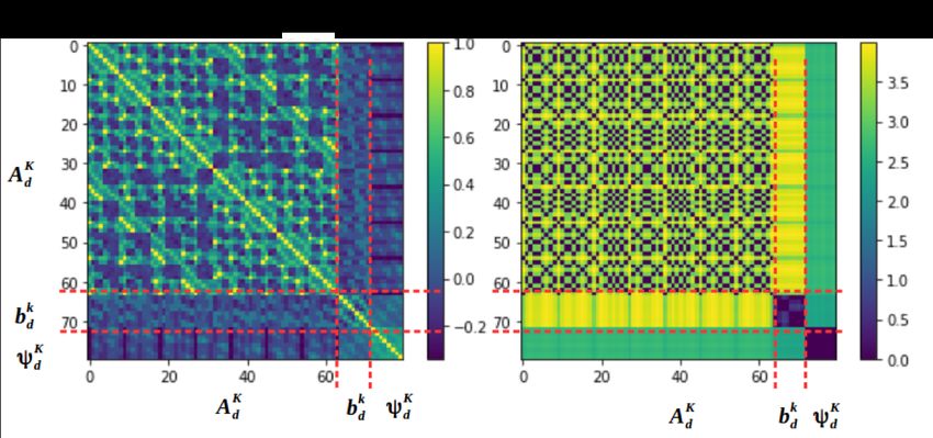
EPJ Web of Conferences 247, 03027 (2021) https://doi.org/10.1051/epjconf/202124703027
PHYSOR2020
one-cell problem, repeated for each phase-space cell, amounts for most of the computational time
in DFEM radiative transport solves. This imposes an upper computational bound on the potential
acceleration of these methods when a fixed computational power is available.
However, when analyzing the local systems obtained for one-cell problems, an underlying structure
can be observed in these systems because of the symmetries and directionality of the radiative
transport process. In the present work, a Machine Learning algorithm is designed to exploit this
structure for accelerating radiation transport solves is presented. The key idea is to replace the
assembly and solution of each local system by a pre-trained ANN recursively evaluated during the
sweeping process.
In the following sections are organized as follows. First, the DFEM discretization of the radiation
transport problem is and the structure appearing in the local systems is analyzed by means of
correlation matrices. Then, the design of a Shallow Neural Network to exploit this structure for
accelerating the solution to one-cell problems is discussed. Finally, key results obtained by mean of
this acceleration are presented.
2. DISCONTINUOUS GALERKIN FINITE ELEMENT METHOD IN TRANSPORT
SWEEPS
The one-group Sn transport equation, with isotropic scattering and sources, is given by
σs φ + q qtot
(Ωd · ∇ + σt )ψd = = (1)
4π 4π
with d the direction
P index in the angular quadrature. The scalar flux is obtained via numerical
integration: φ = d0 wd0 ψd0 , with wd the quadrature weight [2]. For simplicity, in Eq. (1), the total
source (scattering source + extraneous source) has been introduced as the scattering source is often
lagged on iteration behind, and thus merged in with the extraneous source, during a source iterations
process. After the DFEM [3] spatial discretization of Eq. (1), the following local linear system for
cell K in the phase-space (space, direction, energy, and time) is obtained
X 1 X
Ωd · G + σtK M + (Ωd · nf ) S f Ψd = Q+ |Ω · nf | S f Ψd,↑
f (2)
+
4π −
f ∈F f ∈F
where piece-wise constant material properties have been assumed. The set of faces for cell K is split
into faces where radiation is incoming and outgoing, F ∓ = {f ∈ ∂K, s.t., Ωd · nf ≶ 0}. Besides,
Ψ denotes the DFEM solution in the current cell, while Ψ↑f denotes the upwinded flux (transmitted
through faces from the upwind cell neighbors). The local matrices are defined as follows:
Z
ij
G =− bj ∇bi d3 r (3)
Z K
ij
S f = bi bj d2 r (4)
f
Z
ij
M = bi bj d3 r (5)
K
Z
Qi = bi qtot d3 r . (6)
K
2EPJ Web of Conferences 247, 03027 (2021) https://doi.org/10.1051/epjconf/202124703027
PHYSOR2020
The DFEM basis functions on cell K are denoted by bi (r) and (i, j) ∈ [1, N K ] where N K is the
number of spatial degrees of freedom for cell K. The size of the local system is N K × N K . Here,
we restrict ourselves to trilinear basis functions on hexahedral cells, so that N K = 8.
In a more general form, Eq. (2) can be written as
AdK ΨdK = bdK . (7)
where AdK is the matrix of coefficient for the local system and bdK is the right-hand-side vector
containing the incident fluxes and source. During a regular solution process, the right-hand-side bdK
is computed for each cell K, by updating the incident upwinded fluxes and scattering source from
the previous iteration, and, then, system in Eq. (7) is solved by GE. In this case, this results in 729
computational operations. For simplicity, we assume equivalent computational cost in all operations,
although divisions are proven to be more computationally expensive in modern processors [4]. This
is the upper bound when replacing this process with the Machine Learning algorithm.
The base ground to design an accelerator based on a Machine Learning algorithm is to demonstrate
that there exist a structure in problem (7) and, thus, a simpler mapping between inputs (AdK ,
ΨdK ) and output (bdK ) is achievable. In this case, in order to study the system’s structure, a set
random one-cell problems have been generated. When generating each random problem the internal
sources, incident fluxes, total cross section, direction vector, and the cell’s dimensions are randomly
sampled from a uniform random distribution. Then, Eq. (2) is assembled and solved. Finally,
the solution vector bdK is collected for each of these problems. A total of 105 random problems
are necessary to obtain statistical convergence among the second order correlations in each of the
components of the discretized system Eq. (7). Therefore, in the system structure is analyzed in light
of these correlations. In particular Pearson’s correlations and Student’s t-tests are performed as
two complementary statistical measures of correlation among the data. The results obtained for the
correlation coefficients between each of the entries of the system matrix (A), the right-hand-side
vector (b), and the solution vector (Ψ) are presented in Figure 1.
Figure 1: Pearson correlation matrix obtained for a set of 105 random one-cell DFEM
problems.
3EPJ Web of Conferences 247, 03027 (2021) https://doi.org/10.1051/epjconf/202124703027
PHYSOR2020
In Figure 1 it can be obserevd that a large correlation exists among the coefficients in the system’s
matrix. This is a consequence of the way in which this matrix is assembled in Eq. (2) and
because there are more coefficients than random inputs in the system. Moreover, a non-negligible
correlation exists among the components of the right-hand-side vector. This results from the
structure maintained in the construction of the right-hand-side vector (incident fluxes + sources).
Furthermore, structures appear when looking at the correlations of these two with the solution Ψ.
This is evident since the solution vector is univocally determined by the matrix of coefficients and
the right-hand-side vector.
The main conclusion of this section is that there is a structure local systems obtained in the DFEM
discretization of radiation transport. The of next section is to exploit this structure to reduce the
number of operations currently required in the solutions of one-cell problems.
3. MACHINE LEARNING APPROACH FOR ACCELERATING TRANSPORT SWEEPS
The key idea of this work is to replace the assembly and solution by GE of system Eq. (2) with
a shallow Artificial Neural Network (ANN). Note that for a sweeping process the same trained
ANN will be providing the solution for each cell in the phase-space. This means that the sweeping
process is replaced by a staggered recurrent evaluation of the ANN.
The architecture of this ANN is to be optimized in order to reduce the number of operations involved
in its feedforward evaluation, while keeping a bounded error in the solution. The resulting ANN, is
presented in Figure 2. It consists of an ANN with only one hidden layer (shallow ANN). Hyperbolic
tangents have been used as activation functions in the hidden layer, while Exponential Linear Units
(ELUs) has been used as activation functions for the output layer. The reason for first ones is that an
hyperbolic tangent provide the mixed linear-exponential behaviour as a function of its inputs that is
required in the solution to transport problems. Moreover, ELUs can scale the outputs of the ANN
without a bound and, thus, provide the ANN the ability to represent any solution for the angular
fluxes (unlimited positive range). The key part of acceleration arrives when determining appropiate
inputs for the ANN. Rather than feeding in the linear system coefficients (matrix and vector entries),
the input layer takes in as inputs the variables determining the solution of linear system. Specifically,
these are: (i) the incident fluxes over the three incident faces of a sweeping octant (Ψdinc ), (ii) the
total source term in the DFEM nodes within the cell (q), (iii) two independent direction cosines
determining the sweeping angle (µ, η), (iv) the three factors determining the sizes of the hexahedral
cells (∆x, ∆y, ∆z), and (v) the total cross section in the cell (σt ). Thus, the resulting ANN has 26
inputs, instead of the 72 inputs that will be required if the coefficients of the system’s matrix and
right-hand-side vector had been used.
To fundament this idea, a comparison of the number of operations required for the general assembly
and solution by Gauss elimination of system is compared against the number of operations required
for the feed-forward evaluation of the ANN in Figure 3. It is observed that the feed-forward
evaluation of the ANN may allow to reduce the number of operations by a factor of ∼ 3.2, when
using 8 neurons in the hidden layer as shown in Figure 2. The number of neurons in this hidden
layer was set by balancing the ANN fitting error produced by solving local systems with the ANN
versus the acceleration provided by this one.
At this points, three points that differ from classical Machine Learning approaches that are necessary
4EPJ Web of Conferences 247, 03027 (2021) https://doi.org/10.1051/epjconf/202124703027
PHYSOR2020
Figure 2: Concept of feed-forward ANN used in the present study.
to obtain accurate solutions and improve acceleration when building a system based in this ANN: (i)
appropriate definition of a regularized loss function fro training the weights of the ANN, (ii) suitable
algorithm to randomly build the training set avoiding the introduction of biases that can cause
overfitting, (iii) application of an adapted DropConnect that allows accelerating the feedforward
evaluation of the ANN. The first point is discussed here since it is of paramount important in this
work. The reader is referred to out paper [5] for more information on the other two.
The training of the ANNs in each direction is performed on a set of 9 × 10⁴ solutions to one-cell
problems and the testing set consists of 1 × 10⁴ equivalent ones. The training is performed by
backpropagation using the Adam optimization algorithm. For training a testing, the regularized loss
function is defined as follows:
P P 8 P
˜ 1 X kΨd,p − Ψrd,p k1 λ1 X X |Ψd,p,i − Ψrd,p,i | λ2 e−τ 1 X
C= + + kΨd,p − Ψrd,p k1 . (8)
P p=1 kΨrd,p k1 P p=1 i=1 γ1 |Ψrd,p,i | + γ2 τ + γ3 P p=1
where τ is a characteristic optical length of the cell, taken in this case as τ = Σµt ∆ , with the cell size
p
parameter ∆ = ∆x2 + ∆y 2 + ∆z 2 and µ the director cosine in the x̂-direction. Furthermore,
the parameters λ1 , λ2 , γ1 , γ2 , and γ3 are fitted to obtain the required behavior in the ANN. The
values used in this case are presented in Table 1. The first term in the right-hand-side of
Eq. (8) is a classical quadratic loss function. The second one is a Lasso regularization that assigns
higher weights to errors produced by the ANN when the fluxes are small in magnitude. This one is
introduced because large relative errors in small components of the solution vector are hindered in
the classical quadratic definition of the loss function in Eq. (8). In our case, this hindering results
5EPJ Web of Conferences 247, 03027 (2021) https://doi.org/10.1051/epjconf/202124703027
PHYSOR2020
Figure 3: Comparison of the number of operations required for the assembly and solution
by Gauss Elimination of system vs the number of operations required for a feed-forward
evaluation of the ANN.
λ1 λ2 γ1 γ2 γ3
0.15 0.2 10.0 0.01 0.1
Table 1: Parameters used in the regularizer, Eq. (8)
in an error buildup when recurrently evaluating the ANN in a sweeping process. The third term is
also a Lasso regularization parameter that assigns higher values for errors produced in optically thin
problems. This regularizer channels the ANN to find solutions by compressing the inputs in the
hidden layers of the ANN towards zero. The parameters in both regularizing terms have been fitted
after a sensitivity study.
In the following section, the performance of a trained ANN in replacing the solution to one cell
problems is analyzed for a benchmark case.
4. RESULTS
In this paper, we present the results of applying the trained ANNs presented in the previous section
to benchmark Problem 1 proposed in [6]. The geometry of the Benchmark problem is shown in
Figure 4. The problem has one internal source (Region I), followed by a void region (Region II),
and a thick absorber (Region III). The parameters for the three regions are shown in Table 2. This
6EPJ Web of Conferences 247, 03027 (2021) https://doi.org/10.1051/epjconf/202124703027
PHYSOR2020
benchmark case was selected since the ANN could be tested in limiting cases with very different
properties, maximizing the probability of error the buildup in the recurrent evaluation of the ANN
during a transport sweep. The 3D domain was discretized in 100 × 100 × 100 cells. Furthermore,
Figure 4: Geometry of the benchmark used.
4 different ANNs were trained for the S2 , S4 , S6 , and S8 angular quadratures. The average error
for each discretization is shown in Table 3. These errors are larger than the ones obtained during
the training and testing of the ANN for one cell problems (∼ 10−4 ). This indicates that an error
build-up exists when recurrently evaluating the ANN. However, due to the regularizer in Eq. (8)
the error buildup is small enough to yield acceptable solutions. Subsequent work will focused on
techniques to further reducing this error. A large speed-up in computing time is obtained when
employing the ANN. This one is produced by two factors. First, the reduction in the number of
operations required with the ANN (factor 3.2). Then, the most rapid convergence of the solutions
produced with the ANNs during source iterations due to the noise in the connections of the ANN,
which act with a diffusive character when recursively evaluating the network (factor 4.9). The
reader is referred to our paper [5] for more detailed testing cases for this ANN.
Region S [ncm−3 s−1 ] σt [cm−1 ] σs [cm−1 ]
I 1 0.1 0.0999
II 0 10−4 5 × 10⁻⁵
III 0 0.1 0.0999
Table 2: ANN results for the Benchmark problem [6] with c = 0.999.
5. CONCLUSION
In the present work an ANN is proposed for accelerating radiation transport solves. This one
replaces the local system solution for the one-cell problems obtained in the DFEM discretization
of radiation transport. Thus, the sweeping problem to solve radiation transport is replaced by the
recursed evaluation of the ANN. The ANN structure has been optimized by taking a reduced set
7EPJ Web of Conferences 247, 03027 (2021) https://doi.org/10.1051/epjconf/202124703027
PHYSOR2020
Sn Order Mean diff. between Speedup Factor per
ANN & GE Digit Accuracy
2 1.20% 15.8
4 1.83% 15.7
6 2.22% 15.8
8 2.22% 15.8
Table 3: ANN results for the Benchmark problem [6] with c = 0.999
of parameters as inputs that fully determines the solutions to the one-cell problems. Moreover,
accurate solutions are obtained by applying Lasso regularizers to the loss function when training
the ANN. In this paper the results obtained with an ANN trained with 9 × 10⁴ one-cell random
radiative transfer problems and tested on 1 × 10⁴ equivalent ones are presented. This ANN is then
introduced in a large scale 3D problems used as benchmark, where it is observed that replacing
the solution of one-cell problems by the recurrent evaluation of the ANN introduces error between
∼ 1 − 2%, while introducing an acceleration factor of ∼ 15 − 6%. Our future work is oriented to
improving the error in the ANNs, developing hybrid ANN-exact solutions, and using the ANNs as
low order operators in High-Order Low-Order schemes in radiative transfer.
REFERENCES
[1] S. Raschka. “MLxtend: Providing machine learning and data science utilities and extensions to
Python’s scientific computing stack.” J Open Source Software, volume 3(24), p. 638 (2018).
[2] E. E. Lewis and W. F. Miller. “Computational methods of neutron transport.” (1984).
[3] W. H. Reed, T. Hill, F. Brinkley, and K. Lathrop. “TRIPLET: A two-dimensional, multigroup,
triangular mesh, planar geometry, explicit transport code.” Technical report, Los Alamos
Scientific Lab., N. Mex.(USA) (1973).
[4] T. Güneysu and C. Paar. “Ultra high performance ECC over NIST primes on commercial
FPGAs.” In International Workshop on Cryptographic Hardware and Embedded Systems, pp.
62–78. Springer (2008).
[5] M. Tano and J. Ragusa. “Acceleration of Radiation Transport Solves Using Artificial Neural
Networks.” arXiv preprint arXiv:190604017 (2019).
[6] K. Kobayashi, N. Sugimura, and Y. Nagaya. 3-D radiation transport benchmark problems and
results for simple geometries with void regions. Nuclear Energy Agency (2000).
8You can also read