Upstream flow effects revealed in the EastGRIP ice core using Monte Carlo inversion of a two-dimensional ice-flow model
←
→
Page content transcription
If your browser does not render page correctly, please read the page content below
The Cryosphere, 15, 3655–3679, 2021
https://doi.org/10.5194/tc-15-3655-2021
© Author(s) 2021. This work is distributed under
the Creative Commons Attribution 4.0 License.

Upstream flow effects revealed in the EastGRIP ice core using
Monte Carlo inversion of a two-dimensional ice-flow model
Tamara Annina Gerber1 , Christine Schøtt Hvidberg1 , Sune Olander Rasmussen1 , Steven Franke2 , Giulia Sinnl1 ,
Aslak Grinsted1 , Daniela Jansen2 , and Dorthe Dahl-Jensen1,3
1 Section for the Physics of Ice, Climate and Earth, Niels Bohr Institute, University of Copenhagen,
Copenhagen, Denmark
2 Alfred Wegener Institute, Helmholtz Centre for Polar and Marine Research, Bremerhaven, Germany
3 Centre for Earth Observation Science, University of Manitoba, Winnipeg, Canada

Correspondence: Tamara Annina Gerber (tamara.gerber@nbi.ku.dk)

Received: 18 February 2021 – Discussion started: 23 February 2021
Revised: 28 June 2021 – Accepted: 7 July 2021 – Published: 6 August 2021

Abstract. The Northeast Greenland Ice Stream (NEGIS) is            ing are important factors determining ice flow in the NEGIS.
the largest active ice stream on the Greenland Ice Sheet           The results of this study form a basis for applying upstream
(GrIS) and a crucial contributor to the ice-sheet mass bal-        corrections to a variety of ice-core measurements, and the in-
ance. To investigate the ice-stream dynamics and to gain in-       verted model parameters are useful constraints for more so-
formation about the past climate, a deep ice core is drilled       phisticated modelling approaches in the future.
in the upstream part of the NEGIS, termed the East Green-
land Ice-core Project (EastGRIP). Upstream flow can intro-
duce climatic bias into ice cores through the advection of ice
deposited under different conditions further upstream. This is     1   Introduction
particularly true for EastGRIP due to its location inside an ice
stream on the eastern flank of the GrIS. Understanding and         The East Greenland Ice-core Project (EastGRIP) is the first
ultimately correcting for such effects requires information on     attempt to retrieve a deep ice core inside an active ice stream.
the atmospheric conditions at the time and location of snow        The drill site is located in the upstream part of the North-
deposition. We use a two-dimensional Dansgaard–Johnsen             east Greenland Ice Stream (NEGIS; Fahnestock et al., 1993),
model to simulate ice flow along three approximated flow           which is a substantial contributor to the Greenland Ice Sheet
lines between the summit of the ice sheet (GRIP) and East-         (GrIS) mass balance (Khan et al., 2014) and accounts for
GRIP. Isochrones are traced in radio-echo-sounding images          around 12 % of its total ice discharge (Rignot and Mouginot,
along these flow lines and dated with the GRIP and EastGRIP        2012). Large-scale ice-sheet models are essential tools to an-
ice-core chronologies. The observed depth–age relationship         ticipate the future development of the NEGIS and its poten-
constrains the Monte Carlo method which is used to deter-          tial impact on the stability of the GrIS (Joughin et al., 2001;
mine unknown model parameters. We calculate backward-              Khan et al., 2014; Vallelonga et al., 2014). However, results
in-time particle trajectories to determine the source location     obtained from such models often show a significant deviation
of ice found in the EastGRIP ice core and present estimates        from observed surface velocities in the NEGIS and its catch-
of surface elevation and past accumulation rates at the depo-      ment area (Aschwanden et al., 2016; Mottram et al., 2019).
sition site. Our results indicate that increased snow accumu-      In particular, the high ice-flow velocities in the upstream area
lation with increasing upstream distance is predominantly re-      of the NEGIS and the clearly defined shear margins are diffi-
sponsible for the constant annual layer thicknesses observed       cult to reproduce with ice-flow models (Beyer et al., 2018). A
in the upper part of the ice column at EastGRIP, and the in-       recent study by Smith-Johnsen et al. (2020a) showed that the
verted model parameters suggest that basal melting and slid-       high surface velocities in the onset region of the ice stream
                                                                   could be reproduced with their model, using an exceptionally

Published by Copernicus Publications on behalf of the European Geosciences Union.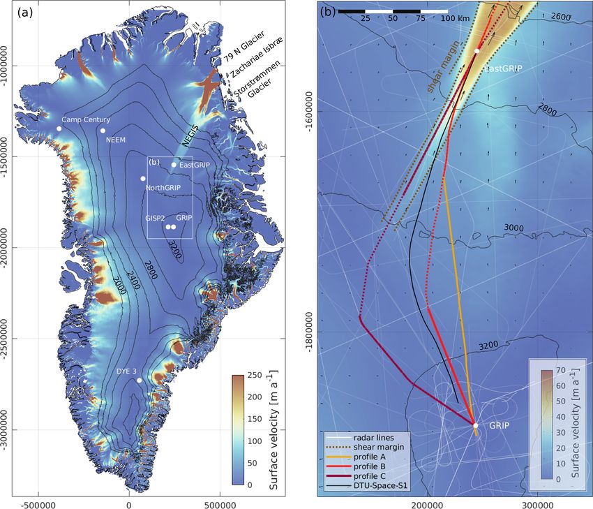
3656                                                       T. A. Gerber et al.: Upstream flow effects in the EastGRIP ice core

high and geologically unfeasible geothermal heat flux (Bons         Greenland’s main ice ridge (Burgess et al., 2010) and the
et al., 2021). This indicates that additional, yet unknown, pro-    increasing elevation towards the central ice divide (Simon-
cesses must facilitate ice flow in the NEGIS and that the driv-     sen and Sørensen, 2017). The correction of these effects in
ing mechanisms governing ice flow are still not understood          the EastGRIP ice core is necessary to interpret the ice-core
well enough. The EastGRIP ice core sheds some light on the          measurements within the climatic context and requires infor-
key processes by revealing unique information about ice dy-         mation on the conditions at the time and location of snow
namics, stress regimes, temperatures and basal properties, all      deposition.
of which are crucial components in ice-flow models.                    Post-depositional deformation of isochrones observed in
   Chemical and physical properties measured in ice cores           radio-echo-sounding (RES) images along flow lines provides
reflect the atmospheric conditions at the time and location of      information on ice-flow dynamics and can be used to recon-
snow deposition (e.g. Alley et al., 1993; Petit et al., 1999;       struct past and present flow characteristics. In this study, we
Andersen et al., 2004; Marcott et al., 2014). Most of the           use a vertically two-dimensional Dansgaard–Johnsen model
deep drilling projects in Greenland and Antarctica are lo-          to simulate the propagation and deformation of isochrones
cated in slow-moving areas at ice domes or near ice divides         along three approximated flow lines between the ice-sheet
(e.g. GRIP – Dansgaard et al., 1982; Dome Fuji – Ageta              summit (GRIP) and EastGRIP. A Monte Carlo method is
et al., 1998; Dome C – Parrenin et al., 2007), so the ice core      used to determine the unknown model parameters by mini-
can be expected to represent climate records from this fixed        mizing the misfit between modelled and observed data. The
location. For ice cores drilled on the flank of an ice sheet        latter includes the depth of isochrones observed in RES im-
(e.g. GISP2 – Meese et al., 1997; Vostok – Lorius et al.,           ages along the flow lines and a parameter αsur representing
1985; Petit et al., 1999) or in areas with higher flow velocities   the sum of the horizontal strain rates deduced from satellite-
(e.g. Camp Century – Dansgaard and Johnsen, 1969; Byrd –            based surface velocities. From the modelled velocity field,
Gow et al., 1968; NorthGRIP – Andersen et al., 2004; EDML           we calculate particle trajectories backwards in time to infer
– Barbante et al., 2006; WAIS Divide – Fudge et al., 2013;          the source location of ice found in the EastGRIP ice core and
NEEM – NEEM Community members et al., 2013), the ice                estimate the accumulation rate at the time of snow deposi-
found at depth was originally deposited further upstream and        tion. The source characteristics presented here form a basis
advected with the horizontal flow.                                  to correct for upstream effects in various chemical and physi-
   The spatial variation in accumulation rate, surface temper-      cal quantities of the EastGRIP ice core. These corrections are
ature and atmospheric pressure can introduce climatic im-           important to remove any climatic bias in ice-core measure-
prints into the ice-core record which stem from the advec-          ments which are currently being analysed and will become
tion of ice deposited under different conditions further up-        available in the future. The inverted model parameters give
stream. The ice core signal is thus a combination of tem-           insight into basal properties and ice-flow dynamics along the
poral and spatial variations in climatic components (Fudge          flow lines and can be used to constrain more sophisticated
et al., 2020). The magnitude of these so-called upstream ef-        numerical models of the NEGIS.
fects depends on the ice-flow velocity, spatial variability in
the precipitation and the sensitivity to atmospheric variations
in the quantity under consideration. While well-mixed atmo-         2   Data and methods
spheric gases, such as carbon dioxide or methane, and dry-
                                                                    Snow layers deposited at the surface of ice sheets are buried
deposited impurities are barely affected (Fudge et al., 2020),
                                                                    with time and are deformed as a consequence of ice flow.
properties extracted from the ice phase can show significant
                                                                    While these isochrones can be observed in RES images to-
bias. Affected measurements include aerosols and cosmo-
                                                                    day, the ice-flow characteristics which shaped them are gen-
genic isotopes, such as 10 Be (Yiou et al., 1997; Finkel and
                                                                    erally unknown. This is a typical geophysical inverse prob-
Nishiizumi, 1997; Raisbeck et al., 2007; Delaygue and Bard,
                                                                    lem and can be formulated as d = g(m), where the func-
2011), the isotopic composition of water (Dansgaard, 1964;
                                                                    tion g(m) represents the ice-flow model linking the model
Jouzel et al., 1997; Aizen et al., 2006), the total air content
                                                                    parameters (m) with the observed data (d). A variety of in-
(Raynaud et al., 1997; Eicher et al., 2016) and ice tempera-
                                                                    verse methods exist to find the model parameters which re-
tures (Salamatin et al., 1998). Processes such as vertical thin-
                                                                    produce the observed data within their uncertainties. Here,
ning of the ice column and firn densification are also influ-
                                                                    we use a Markov chain Monte Carlo method to determine the
enced by upstream effects and have consequences on the an-
                                                                    unknown parameters of a two-dimensional ice-flow model
nual layer thicknesses (Dahl-Jensen et al., 1993; Rasmussen
                                                                    by minimizing the misfit between modelled and observed
et al., 2006; Svensson et al., 2008) and the age difference be-
                                                                    isochrones and strain rates. This allows us to reconstruct the
tween ice and the enclosed air (Herron and Langway, 1980;
                                                                    ice-flow characteristics in the past and to determine the flow
Alley et al., 1982). Upstream effects in the EastGRIP ice core
                                                                    trajectories of the EastGRIP ice.
are expected to be particularly strong due to the fast ice flow
in the upstream area (57 m a−1 at EastGRIP; Hvidberg et al.,
2020), the strong gradient in the accumulation rate across

The Cryosphere, 15, 3655–3679, 2021                                                    https://doi.org/10.5194/tc-15-3655-2021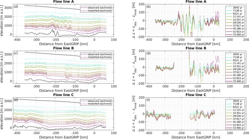
T. A. Gerber et al.: Upstream flow effects in the EastGRIP ice core                                                                     3657

Figure 1. (a) Overview of past and ongoing deep ice-core drilling projects on the GrIS (surface elevation and Greenland contour lines by
Simonsen and Sørensen, 2017; Greene et al., 2017) and the outline of the study area. The NEGIS appears as a distinct feature in the surface
velocities (Joughin et al., 2018). It extends from the central ice divide to the northeastern coast, where it splits up into the three marine-
terminating glaciers: 79N Glacier, Zachariae Isbræ and Storstrømmen Glacier. (b) The present-day EastGRIP flow line is derived from the
DTU-Space-S1 surface velocity product (Andersen et al., 2020). Due to the limited availability of radar data along the flow line, we construct
three approximate flow lines through a combination of various radar products (profile A–C) between GRIP and EastGRIP. Flow line B and C
lack data in the centre of the profiles, marked as a dashed line. The downstream parts of line A and B comprise the same radar profile, which
crosses the southern shear margin around 82 km upstream of EastGRIP.

Table 1. RES profiles used to approximate the EastGRIP flow lines A–C. The data sets were measured between 1999 and 2018 by the
Center for Remote Sensing of Ice Sheets (CReSIS; CReSIS, 2021) and the Alfred Wegener Institute, Helmholtz Centre for Polar and Marine
Research (AWI; Jansen et al., 2020; Franke et al., 2021b).

                             Flow line    Data files                        Institution   Year     Radar system
                             A            Data_20180512_01_001 – 004        AWI           2018     MCoRDS 5
                             A            Data_19990512_01_009 – 010        CReSIS        1999     ICORDS 2
                             B            Data_20180512_01_001 – 004        AWI           2018     MCoRDS 5
                             B            Data_19990523_01_016 – 017        CReSIS        1999     ICORDS 2
                             C            Data_20180517_01_002 – 004        AWI           2018     MCoRDS 5
                             C            Data_20120330_03_008 – 011        CReSIS        2012     MCoRDS 2

https://doi.org/10.5194/tc-15-3655-2021                                                          The Cryosphere, 15, 3655–3679, 2021
3658                                                             T. A. Gerber et al.: Upstream flow effects in the EastGRIP ice core

Table 2. Operating parameters of the radar systems used for data acquisition. Further details can be found in Gogineni et al. (2001), Byers
et al. (2012) and Franke et al. (2021b).

       Parameter                    ICORDS 2                 MCoRDS 2                                 MCoRDS 5
       Bandwidth                    141.5–158.5 MHz          180–210 MHz                              180–210 MHz
       Tx power                     200 W                    1050 W                                   6000 W
       Waveform                     Analogue chirp (SAW∗ )   8-channel chirp (two–three waveforms)    8-channel chirp (three waveforms)
       Sampling frequency           18.75 MHz                111 MHz                                  1600 MHz
       Transmit channels            1                        8                                        8
       Receiving channels           1                        15                                       8
       Range resolution             7.6 m                    4.3 m                                    4.3 m
    ∗ SAW: surface acoustic wave.

Table 3. Characteristics of the traced isochrones connecting the GRIP and EastGRIP ice-core sites. Displayed depths and ages are the average
over the three flow lines. Depth uncertainties include the uncertainty related to the picking process and to the radar range resolution. Age
uncertainties are related to the GICC05 timescale uncertainties and isochrone depths. Figure 7d illustrates the depth and climatic context of
these layers in the EastGRIP ice core, identified with the corresponding layer numbers. The bold layers and the EastGRIP ages were used for
the Monte Carlo inversion and are illustrated with a consistent colour code in Figs. 4, 5 and 7.

                     Layer      GRIP depth [m]      EastGRIP depth [m]    GRIP age [years b2k]    EastGRIP age [years b2k]
                     1                  733 ± 13              421 ± 11               3618 ± 73                  3498 ± 94
                     2                  795 ± 13              471 ± 11               4004 ± 74                  3945 ± 95
                     3                  925 ± 13              573 ± 11               4885 ± 85                  4805 ± 93
                     4                 1217 ± 13              838 ± 11              7178 ± 106                  7139 ± 95
                     5                 1262 ± 13               882±11               7575 ± 107                  7531 ± 95
                     6                 1347 ± 13              968 ± 11              8364 ± 122                 8321 ± 110
                     7                 1374 ± 13              996 ± 11              8637 ± 124                 8600 ± 113
                     8                 1533 ± 13              1153±11             10 407 ± 162               10 365 ± 149
                     9                 1592 ± 13             1208 ± 11            11 209 ± 181               11 140 ± 168
                     10                1663 ± 13             1282 ± 11            12 891 ± 327               12 822 ± 290
                     11                1749 ± 13             1355 ± 11            14 612 ± 281               14 350 ± 206
                     12                2039 ± 13             1704 ± 11            28 633 ± 840               28 522 ± 647
                     13                2193 ± 13             1903 ± 11            38 015 ± 994               37 914 ± 793
                     14                2298 ± 13             2035 ± 11           45 463 ± 1189              45 174 ± 1086
                     15                2395 ± 13             2152 ± 11           52 602 ± 1360              51 920 ± 1240
                     16                        –             2360 ± 11                       –              72 400 ± 1306

   In the coming sections we describe the data and methods                 2.1   EastGRIP flow lines
underlying our results according to the workflow illustrated
in Fig. 2.
                                                                           Determining the exact flow line through the EastGRIP ice-
   In Sect. 2.1–2.3 we explain how the isochrone depth–age
                                                                           core site is important to understanding the flow history of
relationship constraining the Monte Carlo method was ob-
                                                                           the survey area and enables us to reconstruct the location
tained. This involves the selection of RES images approxi-
                                                                           where the ice from the ice core was deposited at the ice-
mating the EastGRIP flow line (Sect. 2.1), extending the ex-
                                                                           sheet surface. For this, we use high-resolution satellite-based
isting chronology of the EastGRIP ice core to the current drill
                                                                           surface velocity products (e.g. Joughin et al., 2018; Gardner
depth (Sect. 2.2), and the tracing and dating of isochrones in
                                                                           et al., 2020; Andersen et al., 2020; see Fig. S1 in the Supple-
the RES data (Sect. 2.3). In Sect. 2.4 the ice-flow model is de-
                                                                           ment) to calculate the upstream flow path. Minor uncertain-
scribed in detail, and in Sect. 2.5 we elaborate on the Monte
                                                                           ties and bias in these data products affect along-flow trac-
Carlo method used for parameter sampling. The section num-
                                                                           ing and lead to deviations between flow lines derived from
bers are displayed in the corresponding steps in Fig. 2.
                                                                           different velocity maps. These deviations become more pro-
                                                                           nounced with increasing distance from the starting point, as
                                                                           the uncertainties propagate along the line and in general be-
                                                                           come larger in slow-moving areas of the ice sheet (Hvidberg
                                                                           et al., 2020). Due to the small bias, we consider the DTU-

The Cryosphere, 15, 3655–3679, 2021                                                              https://doi.org/10.5194/tc-15-3655-2021
T. A. Gerber et al.: Upstream flow effects in the EastGRIP ice core                                                              3659

                                                                        (Paren and Robin, 1975). The latter is the most common re-
                                                                        flector type below the firn (Millar, 1982; Eisen et al., 2006),
                                                                        and because it is related to layers deposited over a relatively
                                                                        short period of time, most internal reflection horizons (IRHs)
                                                                        detected by RES can be considered isochrones.
                                                                           The availability of RES data in the study area is limited,
                                                                        and unfortunately, the flight lines generally do not follow
                                                                        the surface velocity field. We have thus composed three ap-
                                                                        proximated flow lines connecting the EastGRIP (75.63◦ N,
                                                                        35.99◦ W; 2720 m) and the GRIP (72.58◦ N, 37.63◦ W;
                                                                        3230 m) drill sites from the available RES data sets (Fig. 1b).
                                                                        The radar data used in this study (Table 1) were mea-
                                                                        sured by the Alfred Wegener Institute, Helmholtz Centre
                                                                        for Polar and Marine Research (AWI; Jansen et al., 2020;
                                                                        Franke et al., 2021b) and the Center for Remote Sensing of
                                                                        Ice Sheets (CReSIS, 2021). The AWI data were recorded
                                                                        by an eight-antenna-element ultra-wideband radar system
                                                                        (MCoRDS 5) mounted on the Polar 6 Basler BT-67 aircraft,
                                                                        operating at a frequency range of 180–210 MHz (Franke
                                                                        et al., 2020, 2021b). The CReSIS radar data were measured
                                                                        by an ICORDS 2 (1999) and a MCoRDS 2 (2012) radar sys-
                                                                        tem, mounted on a NASA P-3 aircraft, at a frequency range
                                                                        of 141.5–158.5 and 180–210 MHz, respectively. Details of
                                                                        the three radar systems are provided in Table 2.
                                                                           The downstream parts of profile A and B consist of the
                                                                        same flight line, which passes through the EastGRIP drill site
Figure 2. Workflow of the applied steps leading to the results de-      and intersects the southern shear margin around 82 km up-
scribed in Sect. 3. The main steps are described in Sect. 2.1–2.5 and   stream of EastGRIP. Outside the NEGIS, the two lines split
marked with the corresponding numbers in the figure: the observed       up and connect to two different RES profiles. Line B remains
data (d obs ) constraining the Monte Carlo method consist of the αsur   relatively close to the flow direction of the DTU-Space-S1
calculated from the ice surface velocities and the isochrone depths
                                                                        line but has a wide data gap in the centre of the profile. In
along the flow lines. The latter is obtained by approximating the
                                                                        line A, this problem is circumvented by using a radar pro-
EastGRIP flow line with selected RES images (Sect. 2.1), extend-
ing the EastGRIP chronology to the current drill depth (Sect. 2.2),     file connecting directly to GRIP, which deviates from the ob-
and subsequent tracing and dating of isochrones (Sect. 2.3). The it-    served surface flow field by more than 15◦ at some locations.
erative Monte Carlo sampling process is illustrated in the grey box     Profile C follows the NEGIS trunk all the way to the central
(Sect. 2.5) and includes data simulation by a Dansgaard–Johnsen         ice divide and connects to GRIP over the ice ridge without
ice-flow model described in Sect. 2.4.                                  crossing the shear margin. Similarly to flow line B, flow line
                                                                        C contains a substantial data gap between the onset region of
                                                                        the NEGIS and the central ice divide.
Space-S1 (Andersen et al., 2020) line the most likely current              To avoid uncertainties related to the proximity of the
flow line (Fig. 1b). Yet, there is no evidence that the present-        model boundaries, the flow lines were extended more than
day velocity field was the same in the past. A slight shift in          50 km beyond EastGRIP and have a total length of 422
the NEGIS shear margins or the central ice divide, for in-              (line A), 421 (line B) and 480 km (line C). To account for
stance, would have a large effect on the velocity field, and,           any differences in surface elevation or topography between
hence, the determination of the flow line of the EastGRIP ice           RES data from different years, the ice surface reflections of
remains ambiguous.                                                      the radar profiles were aligned to the surface elevation from
   RES data reveal the internal structure of glaciers and ice           ArcticDEM (Porter et al., 2018). The bed topography in the
sheets and provide valuable information on the ice-flow char-           data gaps of the profiles was derived from the BedMachine
acteristics, particularly when recorded parallel to the ice flow.       v3 data set (Morlighem et al., 2017).
The electromagnetic waves used in RES are sensitive to con-
trasts in dielectric properties of the medium in which they             2.2   Extending the chronology of EastGRIP from GS-2
propagate. In ice sheets, these contrasts arise through density               to GI-14
variations in the uppermost part of the ice column (Robin
et al., 1969), changes in the crystal orientation fabric (Har-          The validation of our modelling results and the correct dating
rison, 1973) and impurity layers such as volcanic deposits              of isochrones requires a reliable depth–age scale. The Green-

https://doi.org/10.5194/tc-15-3655-2021                                                      The Cryosphere, 15, 3655–3679, 2021
3660                                                        T. A. Gerber et al.: Upstream flow effects in the EastGRIP ice core

Figure 3. Synchronization between the EastGRIP, NorthGRIP and NEEM ice cores and comparison of match points obtained in this study
with earlier results from Mojtabavi et al. (2020). The annual layer thickness of EastGRIP was computed after transferring GICC05 ages
by linear interpolation to the EastGRIP ice core. The blue curve shows the annual layer thickness obtained by the match points only. The
grey line indicates a high-resolution estimate of annual layer thicknesses at EastGRIP, obtained from the linear interpolation between the
EastGRIP–NorthGRIP match points and assigning the interpolated EastGRIP depths to the NorthGRIP ages.

land Ice Core Chronology 2005 (GICC05; Vinther et al.,                 protocol was applied to reduce problems with confirmation
2006; Rasmussen et al., 2006; Andersen et al., 2006; Svens-            bias and to ensure the reproducibility of the match.
son et al., 2006) is based on annual layer counting in vari-              A total of 138 match points were identified between
ous Greenland ice cores. It has been transferred to GRIP and           1383.84 and 2117.77 m, adding to the previously known 381
other deep drilling sites in Greenland by synchronizing the            match points. The match points between EastGRIP and the
ice cores with each other using horizons of, for example, vol-         other two cores are shown in Fig. 3, representing all the vol-
canic origin (Rasmussen et al., 2008; Seierstad et al., 2014).         canic tie points. The GICC05 chronology was transferred
The upper 1383.84 m of the EastGRIP ice core was drilled               to EastGRIP by linear interpolation of depths between the
between 2015 and 2018 and synchronized with the North-                 match points. The age of the 1383.84 m match point was al-
GRIP ice core in previous work (Mojtabavi et al., 2020).               ready established to be 14 966 years b2k, which is near the
   By 2019, the ice-core drilling progressed down to                   termination of Greenland Stadial 2 (GS-2), with a reported
2122.45 m, allowing us to extend the existing timescale                maximum counting error (MCE) of 196 years (Mojtabavi
from 15 kyr to 49.9 kyr b2k (thousands of years before                 et al., 2020). The age of the deepest match point was estab-
2000 CE). As part of the present study, we identified com-             lished to be 49 909 years b2k, just at the end of Greenland
mon isochrones between EastGRIP, NorthGRIP and NEEM                    Interstadial 14 (GI-14), with an MCE of 2066 years.
to transfer the GICC05 chronology to the part of the East-                As in earlier similar work (e.g. Rasmussen et al., 2013;
GRIP record which is not yet synchronized. This involved the           Seierstad et al., 2014), very few match points were observed
same methods applied to NEEM by Rasmussen et al. (2013)                in the stadials, most clearly seen in Fig. 3 in the long sta-
and to the upper 1383.84 m of EastGRIP by Mojtabavi et al.             dial stages of GS-2 and GS-3. The sparse volcanic signals
(2020). The isochrones chosen for synchronization purposes             within stadial periods should not be attributed to diminished
are mainly volcanic eruptions, which are registered as brief           global volcanic activity but rather to increased deposition of
spikes in the electrical conductivity measurements (ECMs;              alkaline dust that neutralizes volcanic acid, caused by the
Hammer, 1980). The search of common ECM spikes was                     prevailing colder and drier climatic conditions (Rasmussen
performed manually with a strong focus on finding patterns             et al., 2013). The largest distance between match points was
of similarly spaced eruptions rather than single and isolated          observed across GS-2 and GS-3 and spans about 162 m of
events. The MATLAB program “Matchmaker” was used to                    EastGRIP ice.
visualize long data stretches and to evaluate the quality of the
match (Rasmussen et al., 2008). An iterative multi-observer

The Cryosphere, 15, 3655–3679, 2021                                                         https://doi.org/10.5194/tc-15-3655-2021
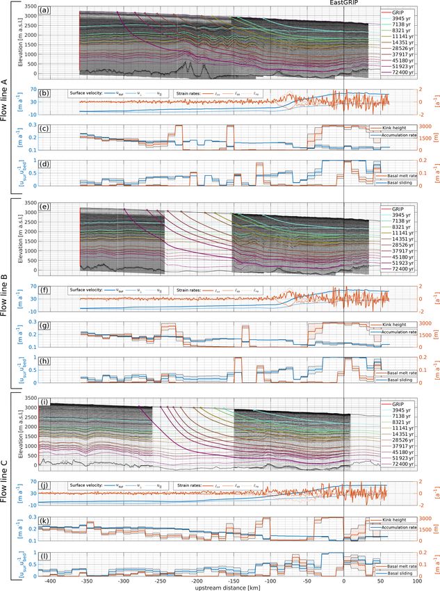
T. A. Gerber et al.: Upstream flow effects in the EastGRIP ice core                                                                        3661

Figure 4. Flow-line characteristics and model parameters for the approximated flow lines A (a–d), B (e–h), and C (i–l). IRHs were traced
(thin solid lines) in the RES images and simulated (dashed lines) with a two-dimensional Dansgaard–Johnsen model (a, e, i). From the
modelled velocity field, we calculated particle trajectories (thick solid lines) backwards in time to obtain estimates of the source location for
specific depths in the EastGRIP ice core. The colours of the lines indicate the age of the isochrones and the respective time of snow deposition
and are identical to the colour code in Figs. 5 and 7. The horizontal strain rates at the surface were calculated from the MEaSUREs Multi-year
v1 (Joughin et al., 2018) surface velocities (b, f, j). The mean and standard deviations of the sampled model parameters accumulation rate,
kink height, basal melt rate and basal sliding (c, d, g, h, k, l) were obtained from a Monte Carlo inversion by reducing the misfit between
observed and simulated data. All panels are aligned at EastGRIP, and the x axis indicates the distance from the borehole location.

https://doi.org/10.5194/tc-15-3655-2021                                                            The Cryosphere, 15, 3655–3679, 2021
3662                                                            T. A. Gerber et al.: Upstream flow effects in the EastGRIP ice core

Figure 5. (a, c, e) Modelled and observed isochrones for profile A–C. The model fits the isochrones well in general but fails to reproduce
strong layer undulations over short distances, leading to a larger misfit (b, d, f) where such undulations are present. A positive misfit indicates
that the modelled isochrone depth is overestimated which happens in particular for the deepest isochrone towards the end of flow line A and
B. As in Figs. 4 and 7, the colour code represents the age of the corresponding isochrone.

2.3     Tracing and dating of isochrones                                    to the radar range resolution (z̃rr ) of the corresponding RES
                                                                            image is defined as
The depth–age relationship from ice-core chronologies can
be extended in the lateral plane by tracing and dating of                              kc
                                                                            z̃rr =     √     ,                                                 (2)
isochrones in RES images. The depth of these isochrones                              2B 3.15
along the EastGRIP flow lines is part of the observed data                  where k is the window widening factor of 1.53, c is the speed
used to tune the ice-flow model parameters in the Monte                     of light, B is the radar bandwidth and 3.15 is the relative
Carlo inversion. We traced 15 continuous IRHs and one non-                  dielectric permittivity of ice.
continuous reflector along each of the three approximated                       The traced IRHs were dated at both drill sites by assign-
flow lines with a semi-automatic MATLAB program called                      ing the reflector depth at GRIP and EastGRIP to the cor-
“picking tool”. The algorithm is based on calculating the lo-               responding timescale. In doing so, local irregularities were
cal slope in each pixel of the RES image, and layers are                    smoothed out by averaging the depth over ±250 m around
traced automatically between two user-defined points. Start-                the trace closest to the ice-core location. Because the East-
ing from each of these points, the algorithm walks along                    GRIP ice core has not reached the bed yet, we extrapolated
the steepest slope towards the other point. Subsequently, the               the timescale at EastGRIP with two IRHs observed below the
two lines are weighted by distance to their starting point and              current borehole depth to obtain a tentative depth–age rela-
combined into one layer. The number of picks required for                   tionship between 2117.77 m and the expected bed depth of
thorough tracing depends on the data quality and reflector                  2668 m.
strength.                                                                       The total age uncertainty (ãt ) was estimated by following
   The total depth uncertainty (z̃t ) was calculated as                     the approach described in MacGregor et al. (2015), where
        q                                                                         q
z̃t =       z̃p2 + z̃rr
                     2 ,                                           (1)      ãt = ãc2 + ãrr
                                                                                           2 + ã 2                                     (3)
                                                                                                 p

where the depth uncertainty introduced during the picking                   takes into account the age uncertainties associated with the
process (z̃p ) is estimated to be 10 m. The uncertainty related             timescale (ãc , equivalent to a 0.5 MCE), the radar range res-

The Cryosphere, 15, 3655–3679, 2021                                                               https://doi.org/10.5194/tc-15-3655-2021
T. A. Gerber et al.: Upstream flow effects in the EastGRIP ice core 3663
olution (ãrr ) and the layer picking process (ãp ). The uncer- approximately equal vertical spacing and used the EastGRIP
tainties related to the range resolution are estimated with ages for our simulation of layer propagation. The layers used
for the Monte Carlo simulation are indicated in bold in Ta-
1X ble 3 and plotted with a consistent colour code in Figs. 4, 5
ãrr = |ac (z ± z̃rr ) − ac (z)| , (4)
2 and 7, representing the corresponding ages.
where ac is the ice-core age from the GICC05 timescale. 2.4 Ice-flow model
Similarly to Eq. (4), ãp is estimated with
A full simulation of ice flow in the catchment area of
1X the NEGIS is a highly under-determined problem (Keisling
ãp = |ac (z ± z̃p ) − ac (z)|. (5)
2 et al., 2014), lacking geophysical, climatic and ice-core data,
The chosen isochrones show distinct patterns which could some of which will become available in the future. Simpler
be identified in all RES images and allowed us to trace models do not solve the problem in detail and are thus com-
isochrones across disruptions and data gaps. Comparison putationally much cheaper. Hence, limited but still useful in-
of the isochrone depths at the ice-core locations obtained formation can be obtained from a simplified treatment of ice
from different RES images permits assessment of the qual- flow (e.g. Dansgaard and Johnsen, 1969; Dahl-Jensen et al.,
ity of the tracing procedure. The high resolution of the radar 2003; Waddington et al., 2007; Christianson et al., 2013;
images recorded in 2018 facilitates isochrone tracing, and Keisling et al., 2014).
the EastGRIP depths obtained from the two different AWI Here, we use a two-dimensional Dansgaard–Johnsen
radar profiles agree to within 1.5 m. At GRIP, the discrep- model (Dansgaard and Johnsen, 1969) to simulate the propa-
ancy between isochrone depths obtained from three differ- gation and deformation of internal layers along approximated
ent radar profiles can be up to 30 m, which is slightly above flow lines between the ice-sheet summit (GRIP) and East-
the combined depth uncertainty related to the picking pro- GRIP. The simplicity of the model makes it well suited for
cess and the resolution of the RES images. A lower-range the Monte Carlo method due to its few model parameters, the
resolution and signal-to-noise ratio in older RES data in- allowance for large time steps and it having an analytical so-
troduce bias into isochrone identification, and although dis- lution (Grinsted and Dahl-Jensen, 2002). The model assumes
tinct isochrones were chosen, a miscorrelation between IRHs ice incompressibility and a constant vertical strain rate down
recorded by different radar systems can not be entirely ex- to the so-called kink height (h) below which the strain rate
cluded. Moreover, the CReSIS profiles do not precisely in- decreases linearly. Basal sliding and melting are included in
tersect at GRIP and deviate from each other. The radar traces the model, and the ice-sheet thickness (H ) is assumed to be
closest to GRIP are thus found at slightly different locations constant in time.
for the three RES images, which explains the higher discrep- We consider a coordinate system where the x axis points
ancy of radar layer depths. along the approximated flow line, the y axis is horizontal and
The isochrone dating was conducted for each profile in- perpendicular to the flow line, and the z axis indicates the
dividually, and the obtained depths, ages and uncertainties height above the bed. The horizontal velocities parallel (uk )
were averaged over the three lines (Table 3). The deepest and perpendicular (u⊥ ) to the profiles are described by Grin-
non-continuous layer which could be identified at EastGRIP sted and Dahl-Jensen (2002) as
uk,sur (x, y) (1 − fbed ) hz + fbed , z ∈ [0, h]
is found at a depth of 2360 ± 11 m and is estimated to be
uk (z) = (6)
72 400 ± 1306 years old. The layer depths of the continu- uk,sur (x, y), z ∈ [h, H ],
ously traced IRHs range from 421 ± 11 to 2152 ± 11 m at the u⊥,sur (x, y) (1 − fbed ) hz + fbed ,
z ∈ [0, h]
EastGRIP location, corresponding to ages of 3498 ± 94 to u⊥ (z) = (7)
u⊥,sur (x, y), z ∈ [h, H ],
51 920 ± 1240 years b2k. Reflectors 1–9 were deposited dur-
where uk,sur and u⊥,sur are the surface velocities parallel and
ing the Holocene. The remaining reflectors are found in ice
perpendicular to the profile and the basal sliding factor fbed
from the Last Glacial Period from which reflector 10 and 11
is the ratio between the ice velocity at the bed and at the
can be attributed to the onset of the Younger Dryas and the
surface.
Bølling–Allerød. The relation between the GRIP and East-
Ice flow in the vicinity of an ice stream is affected by
GRIP depths of the traced IRHs fits well with the GICC05
lateral compression and longitudinal extension, in particu-
timescale (Mojtabavi et al., 2020; Rasmussen et al., 2014),
lar across the shear margins of the NEGIS. We thus intro-
and the ages obtained from the two drill sites agree within ∂u
the uncertainties. We note that the layer dating at EastGRIP duce α = ∂xk + ∂u ⊥
∂y as the sum of the horizontal strain rates.
consistently leads to younger ages than the dating at GRIP, Due to ice incompressibility, we can write α + ∂ω
∂z = 0, where
which is a likely consequence of inaccuracies related to the ω symbolizes the vertical velocity. The x and y dependency
transformation between ice-core and radar depths. in Eqs. (6)–(7) only relates to the surface velocity such that
Due to computational reasons, we did not use all 16 layers αsur represents the horizontal dependency in the equations
for the Monte Carlo inversion but picked 10 isochrones with and can be calculated from the ice surface velocities.
https://doi.org/10.5194/tc-15-3655-2021 The Cryosphere, 15, 3655–3679, 20213664 T. A. Gerber et al.: Upstream flow effects in the EastGRIP ice core
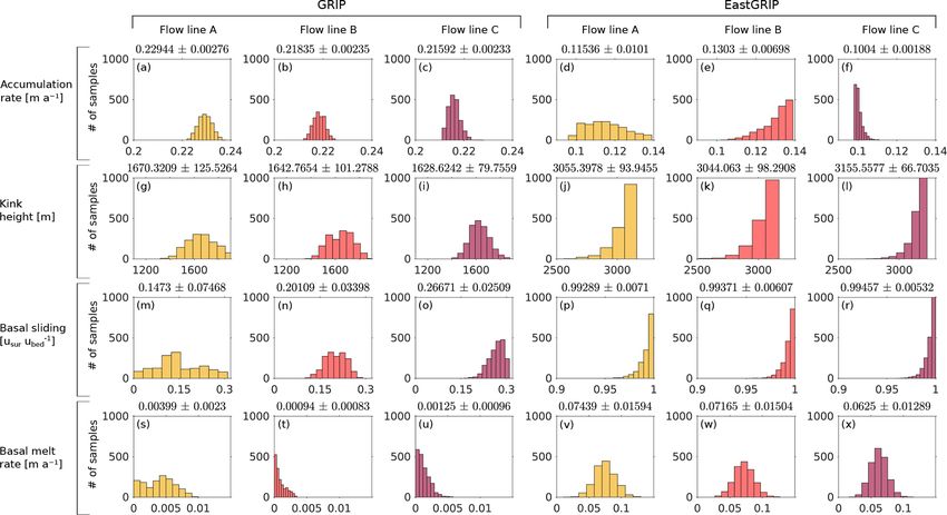
Figure 6. Histograms of the model parameters accumulation rate, basal melt rate, kink height and basal sliding at GRIP and EastGRIP for
each flow line. The corresponding means and standard deviations are displayed on top of the histograms.
cw − cc
The vertical velocities (ω) are obtained through integration with κ1 = and κ2 = cw − δ 18 Ow κ1 .
R
of the incompressibility relation ω(z) = − αdz (Dansgaard δ 18 Ow − δ 18 Oc
and Johnsen, 1969): We use the oxygen isotope δ 18 O record from NorthGRIP
(
z2
(Andersen et al., 2004) due to its high temporal resolution,
ωbed − αsur fbed z + 2h (1 − fbed ) z ∈ [0, h]
ω(z) = and δ 18 Ow = −35.2 ‰ and δ 18 Oc = −42 ‰ are typical iso-
ωsur + αsur (H − z) z ∈ [h, H ]. tope values for warm interstadial and cold stadial periods, re-
(8) spectively. The parameters cw and cc determine the sensitiv-
ity of the accumulation rate with varying δ 18 O in warm (cw )
The boundary conditions for the vertical velocity at the bed
and cold (cc ) periods and are defined as follows (Grinsted
(ωbed ) and surface (ωsur ) are
and Dahl-Jensen, 2002; Buchardt and Dahl-Jensen, 2007):
∂Ebed
ωbed = −ḃ + fbed usur , (9) 1 ∂ ȧ 1 ∂ ȧ
∂x cw = , cc = . (13)
∂Esur ȧ ∂δ 18 O δ 18 O=δ 18 O w
ȧ ∂δ 18 O δ 18 O=δ 18 Oc
ωsur = −ȧ + usur , (10)
∂x
To simulate the propagation of ice particles deposited at the
where ḃ is the positive basal melt rate; ȧ is the positive ac- surface of the GrIS, Eqs. (6) and (8) are solved at a time
cumulation rate; and Ebed and Esur are the bed and surface interval of 10 years.
elevations, respectively. From Eq. (8) we derive the follow-
ing expression for the modelled αsur : 2.5 Monte Carlo sampling
ωbed − ωsur
αsur = . (11) The ice-flow parameters ȧ, h, fbed and ḃ are defined for in-
H − h2 (1 − fbed ) tervals of ∼ 10 km along the flow lines and form together
Following Grinsted and Dahl-Jensen (2002) and Buchardt with the two climate scaling factors, cc and cw , the model
and Dahl-Jensen (2007), we adjust the accumulation rates vector m. This results in a total of 170 (flow line A and B)
and surface velocities to the climate conditions of the cor- and 194 (flow line C) model parameters. Each combination
responding time with a scaling factor ξ(t): of them represents a possible solution to the inverse prob-
1
lem d = g(m), where g(m) represents the ice-flow model de-
18 O−δ 18 O 18 2 18 2
ξ(t) = eκ2 (δ w )− 2 κ1 (δ O −δ Ow ) , (12) scribed in the previous section. The data vector d contains the
The Cryosphere, 15, 3655–3679, 2021 https://doi.org/10.5194/tc-15-3655-2021T. A. Gerber et al.: Upstream flow effects in the EastGRIP ice core 3665
Figure 7. Modelled upstream distance (a) and surface elevation (b) of the source location for ice in the EastGRIP ice core. The thinning
function (c) was calculated from the modelled accumulation rates and annual layer thicknesses (d) and was combined with the interpolated
annual layer thicknesses observed in the ice core (d) to calculate past accumulation rates in high resolution (e). The δ 18 O curve from
NorthGRIP (f) was scaled to the EastGRIP depths to put the results into a climatic context. The depths of the traced isochrones from Table 3
are displayed with the same colour index as in Figs. 4 and 5 and labelled with the corresponding layer number.
isochrone depths and αsur determined from the MEaSUREs To estimate the initial accumulation rate ȧ0 , we integrate
Multi-year v1 surface velocities (Joughin et al., 2018) at a Eq. (8) (see Appendix B) and obtain the following depth–age
resolution of 1 km. relationship
Like in most geophysical inverse problems, many different
combinations of model parameters can explain the observed ȧ
(H − z) = (1 − e−αsur t ), (14)
data equally well within the range of their uncertainties, and αsur
therefore, a non-unique solution does not exist. Probabilis-
where t and z represent the isochrone age and height above
tic inverse methods consider many different models and de-
the bed, respectively. The accumulation rate ȧ is determined
scribe them in terms of their plausibility, rather than find-
with a curve-fitting function, using at least five isochrones
ing one possible solution. This makes these methods partic-
younger than 10 kyr at each point along the flow line. The ini-
ularly well suited for nonlinear problems, where the prob-
tial kink height (h0 ), basal sliding (fbed,0 ) and basal melt rate
ability density in the model space typically shows multiple
(ḃ0 ) are scaled with the normalized surface velocity (ûsur ) as
maxima (Mosegaard and Tarantola, 1995).
follows:
Monte Carlo methods are based on a random number gen-
erator which allows the sampling according to the target
1
probability distribution in an efficient way. The grey box h0 = H − e1 ûsur , (15)
2
in Fig. 2 illustrates the iterative sampling process of the
fbed,0 = e2 ûsur , (16)
Metropolis algorithm (Metropolis et al., 1953) used here:
starting from an initial model (m0 ), a random walker explores ḃ0 = e3 ûsur , (17)
the model space and proposes new models (mnew ) which are
accepted with a certain probability (Paccept ). This way of im- where e1 = 0.4, e2 = 0.8 and e3 = 0.03 and the initial value
portance sampling avoids unnecessary evaluation of model for cw and cc is assumed to be 0.15 and 0.10, respectively. In
parameters in low-probability areas (Mosegaard, 1998). each iteration a new model mnew is proposed as
mnew = m0 + qA, (18)
https://doi.org/10.5194/tc-15-3655-2021 The Cryosphere, 15, 3655–3679, 20213666 T. A. Gerber et al.: Upstream flow effects in the EastGRIP ice core
where m0 is the initial model and A contains the perturbation Table 4. Perturbation amplitude (A) and step length (p) of the in-
amplitude of the corresponding model parameters. The vec- dividual model parameters used for the Monte Carlo sampling. The
tor q defines the random walk in the multidimensional model sampling parameters were chosen such that the acceptance ratio of
space and solely depends on the preceding step. In each iter- the individual model parameters lies between 25 % and 75 %.
ation, i, one model parameter, j , is randomly selected and
perturbed as Model parameter Amplitude (A) Step length (p)
ȧ 0.01 m a−1 0.5
1
q i+1 (j ) = q i (j ) + r − p(j ), (19) ḃ 0.01 m a−1 1
2 h 100 m 3
where r indicates a random number between 0 and 1 and p fbed 0.05 2
cc 0.05 0.5
regulates the maximum step length per iteration of the se-
cw 0.05 0.5
lected parameter type. To achieve a good performance of the
Monte Carlo algorithm, the values of A and p (shown in Ta-
ble 4) are chosen such that the acceptance ratio for the indi-
vidual model parameters lies between 25 % and 75 %. 3 Results
The quality of the proposed model is evaluated by the
function S(m) which describes the misfit between the mod- 3.1 Model parameters
elled and observed data (see Appendix C). The new model
(mnew ) is accepted with the acceptance probability (Metropo-
Due to the mixed determined nature of the inverse problem
lis et al., 1953)
addressed in this study, a unique solution of model param-
eters does not exist. The Monte Carlo sampling results in a
L(mnew )
Paccept = min ,1 , (20) number of possible models distributed according to the pos-
L(mold )
terior probability. Here, we present the mean model parame-
where mold is the last accepted model and the likelihood ters with the standard deviations of the posterior probabil-
function is defined as L(m) = e−S(m) . ity distribution and emphasize that the corresponding his-
To ensure that parameter sampling is occurring in a physi- tograms (Fig. 6) are essential to understanding the uncertain-
cally reasonable range, the a priori probability distribution is ties in the parameter considered.
assumed to be uniform within the following intervals: The flow-line characteristics and model parameters for
h i each flow line are summarized in Fig. 4. The radar profiles
ȧ ∈ ȧ0 − 0.02 m a−1 , ȧ0 + 0.02 m a−1 , (21) with the observed and modelled isochrones are displayed as
a function of the distance from the EastGRIP ice-core loca-
h ∈ [0, H ] , (22)
tion. Particle trajectories were calculated from the simulated
fbed ∈ max(0, fbed,0 − 0.3), min(1, fbed,0 + 0.3) , (23) velocity field with the mean model parameters and indicate
h i
ḃ ∈ 0, 0.2 m a−1 . (24) the source location of ice found at the modelled isochrone
depth in the EastGRIP ice core. The isochrones and particle
The sampling intervals are based on expected values of the trajectories are illustrated with the same colour code as in
corresponding parameter: the initial accumulation rate ob- Figs. 5 and 7f, indicating the corresponding age. The hor-
tained from the radar stratigraphy is considered quite trust- izontal strain rates (ε̇xx , ε̇yy and ε̇xy ) were obtained from
worthy, but because the local layer approximation is not justi- the MEaSUREs Multi-year v1 surface velocity components
fied in the survey area (Waddington et al., 2007) we allow the (Joughin et al., 2018) parallel (uk ) and perpendicular (u⊥ ) to
accumulation rate to deviate by 0.02 m a−1 . The kink height the approximated flow line. The strain rates show mostly low,
is limited to the ice-sheet thickness; the basal sliding fraction positive values along the flow lines with the exception of the
is allowed to deviate by 30 % from the initial model, and the shear-margin crossing in profile A and B, which is character-
upper limit of the basal melt rate is based on values suggested ized by longitudinal extension and lateral compression.
at EastGRIP by a recent study (Zeising and Humbert, 2021). The central observed features are the following:
In their initial phase, Markov chain Monte Carlo methods
move from the starting model towards a high-probability area 1. The accumulation rate decreases with increasing dis-
where the target distribution is sampled. To avoid sampling tance from the central ice divide. In flow line A and B,
during this so-called burn-in phase, the first 1×10⁶ accepted it remains almost constant between −220 and −80 km,
models are discarded. Since only one parameter is perturbed followed by a drop of about 20 % across the shear mar-
at a time, successive models are highly correlated. To obtain gins. In the first ∼ 150 km of flow line C, which corre-
a distribution of independent models, only every 1000th ac- sponds to the ice divide, the accumulation rate remains
cepted model is saved. The sampling is continued for 6×10⁶ nearly constant, followed by a gradual decrease with in-
iterations in total. creasing distance along the profile.
The Cryosphere, 15, 3655–3679, 2021 https://doi.org/10.5194/tc-15-3655-2021T. A. Gerber et al.: Upstream flow effects in the EastGRIP ice core 3667
2. The kink height fluctuates around the middle of the ice 3.3 Ice origin and ice-flow history
column in the vicinity of the ice ridge and is drawn
closer to the bed in the centre of the profiles. Locally From the modelled velocity field, we calculate particle tra-
very high kink heights are observed in flow line A jectories backwards in time (Fig. 4) which give insight into
around −230 and −150 km, in flow line B at −240 and the source location and flow history of ice found at a certain
−140 km, and at −100 km in flow line C. In all profiles, depth in the EastGRIP ice core and allow us to determine
h increases substantially at about −60 km. the accumulation rate during its deposition (Fig. 7e). Due to
the higher velocities in the ice stream, the ice source loca-
3. The basal velocity ranges between 0 % and 50 % of the tion in the upper 1600 m of the ice core lies further upstream
surface velocity outside the NEGIS and increases to for flow line C compared to flow line A and B. For deeper
60 %–100 % in the vicinity of EastGRIP. ice, this trend is reversed, as the velocity along flow line C
drops below the velocity of line A and B (Fig. 7a). A sim-
4. The basal melt rate at the beginning of the profiles varies
ilar effect manifests itself in the upstream elevation, where
between 0 and 0.03 m a−1 . As for the kink height, flow
higher velocities along flow line C result in higher elevations
line A shows strong melt rate fluctuations in the centre
in the upper part of the ice column, which is compensated
of the profile, some of which are also observed in flow
for by a flatter topographic profile for ice deeper than 1400 m
line B. At EastGRIP, basal melt rates of between 0.05
(Fig. 7b).
and 0.1 m a−1 are obtained, but higher values of up to
From the model-inferred in situ accumulation rates, ȧm ,
0.2 m a−1 are reached further downstream.
and annual layer thicknesses, λm , we calculate the ice-core
thinning function γ :
3.2 Monte Carlo performance
ȧm − λm
γ= . (25)
The comparison of modelled and observed isochrones ȧm
(Fig. 5a, c, e) and αsur (Fig. S2 in the Supplement) shows
a good fit in most parts of the flow lines. However, our model The thinning function increases nearly linearly with depth
is not able to accurately reproduce strong internal layer un- in the Holocene and shows a considerable decrease in
dulations which are not related to the bed topography or the the Younger Dryas and enhanced thinning in the Bølling–
surface conditions, resulting in a larger misfit where such un- Allerød. In the glacial part of the ice core, the thinning func-
dulations are present (Fig. 5b, d, f). In general, the isochrone tion fluctuates between interstadials and stadials. The shift
misfit tends to be larger for deeper layers. Particularly dis- between the three lines results from the slightly different
tinct is the positive misfit at EastGRIP for the deepest layer in depth–age relationships and isochrone misfits obtained from
all profiles, indicating that the depths of old layers are over- the three profiles. We combine the thinning function with the
estimated. The average isochrone misfit for flow line A, B annual layer thicknesses observed in the EastGRIP ice core,
and C is 2.94 %, 2.34 % and 1.49 % of the respective layer λobs , to estimate past accumulation rates, ȧpast :
depth.
λobs
Histograms in Fig. 6 show the sampled probability dis- ȧpast = . (26)
tribution of model parameters at GRIP and EastGRIP with 1−γ
the corresponding mean and standard deviation displayed on We find that the accumulation rate at the deposition site in-
top. Distributions with distinctive single peaks and low stan- creases from ∼ 0.12 m a−1 to a maximum of 0.249 m a−1 for
dard deviations point towards a good parameter resolution, ice at a depth of 912 m, which was deposited approximately
while multiple maxima or large standard deviations indicate 7800 years b2k. We note that the constant annual layer thick-
that several models are found to be equally likely. The pa- nesses observed in the upper 900 m of the EastGRIP ice core
rameter resolution is in general better at the beginning of (Mojtabavi et al., 2020) coincide with the spatial pattern of
the profiles, most clearly represented by the narrow distri- increasing accumulation along the flow line with increasing
butions in the accumulation rate, basal melt rate and kink upstream distance (Figs. 4c, g, k and 7d, e). Ice between
height at GRIP. Exponential distributions imply that a param- 900 and 1400 m is characterized by the transition from the
eter reaches regularization boundaries. This is the case for the Holocene into the Last Glacial Period with decreased accu-
basal melt rates at GRIP, the kink height and basal sliding mulation rates in the Younger Dryas and a peak during the
factor at EastGRIP, and the accumulation rate in flow line B Bølling–Allerød (Fig. 7e). The accumulation rate at the depo-
and C at EastGRIP. The climate parameter cw is found to be sition site for older ice varies between 0.02 m a−1 during sta-
0.10±0.005 for all flow lines. The obtained value for param- dials and 0.196 m a−1 during interstadials. The atmosphere in
eter cc is 0.14±0.003 for flow line A and B and 0.16±0.004 the glacial period was in general colder and dryer, and hence,
for flow line C. The histograms of cw and cc can be found in accumulation rates were typically lower than today (Cuffey
Fig. S3 in the Supplement. and Clow, 1997). However, due to the upstream flow effects,
the ice from the interstadials could have been deposited under
https://doi.org/10.5194/tc-15-3655-2021 The Cryosphere, 15, 3655–3679, 20213668 T. A. Gerber et al.: Upstream flow effects in the EastGRIP ice core
Table 5. Essential quantities for upstream corrections for selected depths of the EastGRIP ice core. The upstream distance, elevation and past
accumulation rates ȧpast describe the characteristics of the source location and the conditions during ice deposition. ȧpresent represents the
corresponding present-day accumulation rates at the source location. All quantities are averages over the three flow lines, and the uncertainties
represent the maximum deviation from the mean.
Depth Age Upstream distance Elevation Thinning function ȧpast ȧpresent
[m] [years b2k] [km] [m a.s.l.] [m a−1 ] [m a−1 ]
100 665 47 ± 3 2752 ± 10 0.10 ± 0.03 0.12 ± 0.004 0.12 ± 0.015
200 1553 74 ± 2 2788 ± 11 0.19 ± 0.08 0.14 ± 0.006 0.14 ± 0.005
300 2418 92 ± 1 2837 ± 14 0.16 ± 0.05 0.13 ± 0.005 0.15 ± 0.010
400 3322 105 ± 7 2854 ± 6 0.21 ± 0.02 0.14 ± 0.002 0.14 ± 0.031
600 5037 126 ± 12 2892 ± 14 0.28 ± 0.00 0.16 ± 0.001 0.16 ± 0.005
800 6805 146 ± 14 2920 ± 9 0.35 ± 0.03 0.15 ± 0.005 0.16 ± 0.003
1000 8640 165 ± 13 2944 ± 15 0.42 ± 0.03 0.16 ± 0.004 0.17 ± 0.002
1200 11 015 183 ± 12 2965 ± 19 0.41 ± 0.06 0.12 ± 0.010 0.17 ± 0.005
1400 15 571 200 ± 7 2993 ± 7 0.46 ± 0.01 0.05 ± 0.001 0.17 ± 0.015
1600 23 382 217 ± 3 3027 ± 26 0.52 ± 0.08 0.05 ± 0.007 0.18 ± 0.023
1800 33 524 234 ± 8 3054 ± 40 0.72 ± 0.06 0.11 ± 0.028 0.19 ± 0.021
2000 43 107 252 ± 14 3079 ± 54 0.73 ± 0.07 0.10 ± 0.019 0.19 ± 0.022
2200 54 864 271 ± 19 3108 ± 73 0.83 ± 0.02 0.07 ± 0.006 0.19 ± 0.030
2400 75 980 293 ± 18 3136 ± 80 0.83 ± 0.11 0.08 ± 0.034 0.19 ± 0.023
2600 94 696 322 ± 12 3171 ± 67 0.94 ± 0.03 0.18 ± 0.044 0.20 ± 0.005
higher accumulation rates than are observed at the EastGRIP and basal sliding lead to depth-dependent deformation of the
site today. isochrones (Keisling et al., 2014).
The variations in the past accumulation-rate between the The accumulation rates of ∼0.21–0.23 m a−1 at GRIP and
three flow lines result from both the varying along-flow ac- ∼0.1–0.13 m a−1 at EastGRIP obtained in this study agree
cumulation pattern and different upstream distances of the with field observations (Dahl-Jensen et al., 1993; Vallelonga
source location. The spread between the three models pro- et al., 2014), and the low standard deviations point towards
vides important uncertainty estimates. The average deviation a robust solution. In profiles A and B we observe ∼ 20 %
from the mean accumulation rates is 3.9 % in the Holocene lower accumulation rates inside the ice stream than outside.
and 20 % in the Last Glacial Period. The largest spread be- This agrees to some extent with Riverman et al. (2019), who
tween the three flow lines is 68 % observed at a depth of found 20 % higher accumulation rates in the shear margins
2411 m. We remark that, due to missing direct information compared to the surroundings, although our observations are
on the annual layer thicknesses, accumulation rates below not confined to the shear margins only. Regularization on the
the current borehole depth of 2122.45 m are based on tenta- accumulation rate was necessary in our model to avoid unre-
tive estimates and must be treated accordingly. alistically strong fluctuations along the flow lines.
The bed topography and bed lubrication have a consider-
able effect on ice-flow parameters. Flow over bed undula-
4 Discussion tions affects the elevation of internal layers due to variations
in the longitudinal stresses within the ice (Hvidberg et al.,
4.1 Isochrone deformation and ice-flow parameters 1997) and is often reflected in the surface topography (Cuf-
fey and Paterson, 2010). If the bed is “sticky”, i.e. the basal
Deformation of IRHs occurs as a consequence of bed to- sliding is small, the ice is compressed along the flow direc-
pography (Robin and Millar, 1982; Jacobel et al., 1993), tion while vertically extended (Weertman, 1976) and IRHs
spatial variations in basal conditions (Weertman, 1976; are pushed upwards. At a slippery bed, the opposite is the
Whillans, 1976; Whillans and Johnsen, 1983; Catania et al., case, resulting in along-flow extension of IRHs which leads
2010; Christianson et al., 2013; Leysinger Vieli et al., to thinning and thus decreasing distance between the IRHs.
2018; Wolovick et al., 2014), spatially varying accumula- Keisling et al. (2014) argued that major fold trains existing
tion rates and corresponding changes in ice-flow geometry independently of bed undulations can be explained by varia-
(Dansgaard and Johnsen, 1969; Weertman, 1976; Whillans, tions in the basal sliding conditions. This is, for instance, ob-
1976; Whillans and Johnsen, 1983), and convergent ice flow served across shear margins, where local, steady-state folds
and ice-stream activity (Bons et al., 2016). Areas of en- are formed as a response to the basal conditions (Keisling
hanced basal melt rates similarly drag down all the layers et al., 2014; Holschuh et al., 2014). In flow line A, we ob-
above, while variations in accumulation rate, kink height
The Cryosphere, 15, 3655–3679, 2021 https://doi.org/10.5194/tc-15-3655-2021You can also read


